Solving Basic Inventory Models Using Excel

(1)

ISSN Online: 2162-2086 ISSN Print: 2162-2078

DOI: 10.4236/tel.2018.811137 Aug. 6, 2018 2095 Theoretical Economics Letters

Solving Basic Inventory Models Using Excel

Sarbjit Singh

Institute of Management Technology, Nagpur, India

Abstract

In this note, I have introduced a simple way to solve the four basic inventory models using Microsoft excel. This note can be used in courses like econom-ics, operations management, operations research, supply chain management. This note can be used in teaching basic inventory models to avoid the lengthy manual calculation involved in solving them. It can also be used as an inter-esting example for an advanced class in Excel. The user just needs to enter the data in the white cells and all the results are automatically calculated. We recommend showing students how to first solve the models by hand (not necessarily the example problem), so that they understand the procedure, and then show them how to do it using Excel. The four models considered here are EOQ model, Basic production model, Discount Model and Shortage Model. Using the excel managers would be able to compare the various sce-narios provided by the organization. They would find it very convenient to use these models.

Keywords

EOQ Model, Production Model, Shortage Model, Discount Model

1. Introduction

Inventory management involves decisions about the level of inventory, organi-zation should keep to get the maximum profit. Inventory has been defined as

idle resources that possess economic value by Monks [1]. To meet demand on

time, companies often keep on hand stock that is awaiting sale. The purpose of inventory management is minimizing the cost associated with keeping inventory and meeting customer expectations. The two basic questions of inventory man-agement are: 1) When should an order be placed for an Item? 2) How large should each order be?

Economic order quantity model was first developed by Ford Harris [2], but R. H. Wilson [3] applied it extensively, that is, why this is also known as Harris and

How to cite this paper: Singh, S. (2018) Solving Basic Inventory Models Using Excel. Theoretical Economics Letters, 8, 2095-2102. https://doi.org/10.4236/tel.2018.811137

Received: May 31, 2018 Accepted: August 3, 2018 Published: August 6, 2018

http://creativecommons.org/licenses/by/4.0/

(2)

DOI: 10.4236/tel.2018.811137 2096 Theoretical Economics Letters

ing EOQ formula even it has some unrealistic assumptions. David Piasecki [7]

formulated how to optimize cost using EOQ and also deal with conflict between JIT and EOQ.

This article deals with the solution of some elementary inventory models. The note deals with the basic EOQ and its extensions. In this note I have introduced the basic models and also given their excel programs so by using this programs, students can solve the inventory related issues by applying the various elemen-tary models. The programs developed are user friendly and various inventory related problems can be solved using them.

2. The Advantages of Having Large Inventory

Earlier most of the organizations used to keep large inventories. As it has lots of benefits, one of the main reasons was unhampered production. Also buying items in bulk help organizations to get better discounts. Even transportation cost reduces if items are bought in bulk. The customer satisfaction increases as ser-vices would be smooth and faster. Some time it also helps in case of items which are seasonal items, hence helps in price speculations.

3. The Disadvantages of Having a Large Inventory

Like every coin has two sides, keeping large inventory also has numerous disad-vantages. To keep a large inventory, a lot of money is invested which can be used for some other purpose. To keep a large inventory, a lot of money is spending on warehouse rent, accounting and insurance. Also, many items start deteriorating after some time. Some of the items become obsolete after some fixed time.

4. Economic Order Quantity Model

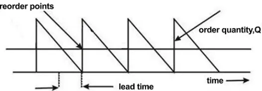
The EOQ model is the elementary model and has the following assumptions. The demand is deterministic and constant over time. Shortages are not allowed, the Lead time is either zero or constant. Order quantity is instantaneous (Figure 1).

S—Cost of placing order; D—Annual demand; H—Annual per-unit carrying

cost; Q—Order quantity; Annual Ordering Cost = S * D/Q; Annual Carrying Cost= H * Q/2; Total Inventory Cost= S * D/Q + H * D/2; Number of Orders =

D/Q; Average Inventory = Q/2.

(3)

[image:3.595.241.504.86.178.2]

Figure 1. Inventory order cycle of EOQ model.

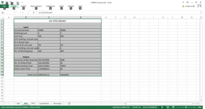
ordering cost per order is $5 and the carrying cost is 0.025 of the average inven-tory value. The price of a single unit is two hundred. The company presently has a policy of placing ten orders every year: Advise the management of Monu Tractors as to whether it should continue with its present policy or switch over to EOQ model.

Here D = 50000; Ordering Cost = $5; Carrying Cost = 2.5%; Cost Price $200. The model built here has considered both the cases i.e. carrying cost is con-stant or dependent on the holding cost.

Excel Program of Economic Order Quantity Model (Figure 2 and Figure 3).

Assumptions

It’s an extension of EOQ model, in this, items are not received instantaneous-ly. Supposition that Order quantity is received all at once is relaxed. The demand of the item is not high enough to warrant continuous production. Therefore items are produced in lots or batches.

p—Daily production rate; d—Daily demand rate; D = Annual Demand; Cs

= Set up Cost; Cc = Carrying Cost.

Annual Production rate (P) is more than the annual demand (D).

Maximum inventory level at any time in the production cycle is given by

Q—Q d p Q∗ =

(

1−d p

)

Mean Inventory Level is given by

(

1

)

.

2

Q ₋_{d p}

Optimal Production Quantity = 2 .

1 s opt C C D Q d C p =   −    

Like previous model, total cost is sum of the set up cost and holding cost

Total Cost= 1

2

s c

C D C Q d

Q p

 

+ _ − _

 

(4)

[image:4.595.211.538.69.242.2]

Figure 2. Solution using excel for case I (Example of EOQ Model).

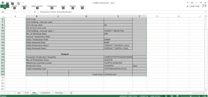
Figure 3. Economic production quantity.

Here Annual Demand is 2 million, the holding cost is ten dollars per bottle per year, the cost of setting up the production is $1000 and daily production p = 10,000 bottles and daily demand = 6000 bottles.

The model built has considered both the cases of carrying cost i.e. it is con-stant or dependent on the price of the item.

Excel Program for solving Production Quantity Model (Figure 4 and Figure 5). In most of the practical scenarios the unit cost of an item is dependent on the quantity procured. Mostly, discounts are offered for the purchase of large quan-tities. These discounts take the form of price breaks.

Price per unit decreases as order quantity increases. In this case total cost includes the purchasing cost also.

First step is to check the EOQ by using the EOQ formula and then check the total cost at the price breaks, whichever gives the lowest the optimal ordering quantity. Here p is the cost price and D is the annual demand.

[image:4.595.210.540.275.450.2]

(5)

[image:5.595.208.539.69.224.2] [image:5.595.208.543.261.434.2]

Figure 4. Solution of the case II using excel program.

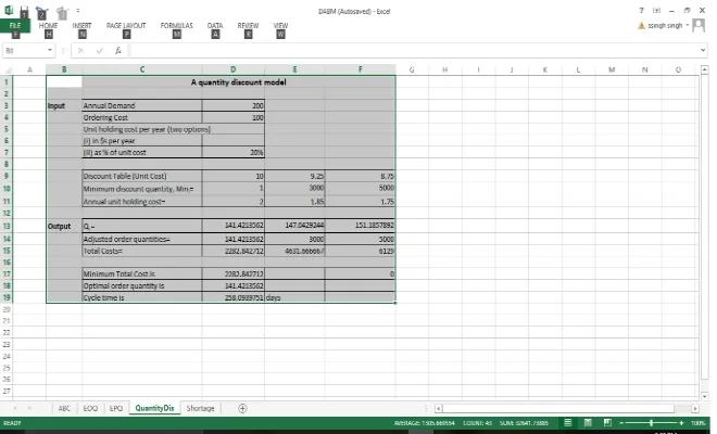
Figure 5. Quantity discount model.

Case III A factory needs 200items, carrying cost = 20%, ordering cost= $100. Price break:

0 - 2999; $10; 3000 - 5000; $9.25; 5000 & above; $8.75.

Find the optimal lot size and the total inventory cost.

Excel Program for solving quantity discount model (Figure 6 and Figure 7). In this model is demand is constant over the finite time horizon and supply is instantaneous. Shortages are allowed and are fully backlogged

Q = total demand per production run

Here in this model one more cost is involved i.e. shortage cost. The shortage cost is denoted by Csh

Optimal Ordering Quantity = 2 o c sh

opt

c sh

DC C C Q

C C

+ =

Maximum Inventory Level = sh

opt

sh c

C M Q

C C

 

= _ _

+

(6)

[image:6.595.210.541.66.247.2] [image:6.595.210.540.280.480.2]

Figure 6. Solution of the case III using excel program.

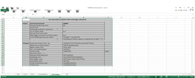
Figure 7. Deterministic Inventory problem with allowable shortages.

Allowable Shortages are given by S Q= _opt−M.

Total Inventory Cost is the sum of ordering cost, holding cost and shortage cost.

Total Inventory Cost = 2 ( )2

2 2

sh opt

o c

opt opt opt

C Q M DC C M

Q Q Q

−

+ +

Case IV:

A dealer has to supply his customer 24,000 units of his product every year. The demand is fixed and known. The penalty of not meeting the demand is twenty cents per month. The inventory holding cost is ten cents per unit per month and the ordering cost is $350 per order. Find the optimal order quantity with allowable shortages. The allowable shortages and the total cost. Also com-pare with the EOQ model.

(7)

[image:7.595.209.538.60.192.2] [image:7.595.208.543.225.361.2]

Figure 8. Solution of case IV considering allowable shortages.

Figure 9. Concluding remarks.

The excel programs given above would help the students to do the analyses of the various situations. For example comparison of the company present policy with applicable inventory model. Whether the company should opt for the dis-count offered by the supplier. It would be a wise decision to produce the item or outsource. Also, companies should go for shortages or not. Thus, by making the above programs, students can do analysis at a faster and easier way. The pro-grams considered above have tried to cover all the aspects of the Inventory mod-el like it provided the option whether carrying cost is constant or dependent on the average inventory. Similarly, daily demand and production rate is given or annual demand and production rate. Accordingly the model can calculate the daily demand and production rate. First student should be introduced to the ba-sic models and then they should be provided these excel programs to do further analysis.

Conflicts of Interest

The authors declare no conflicts of interest regarding the publication of this pa-per.

References

[1] Monks, J.G. (1987) Operations Management. 3rd_{Edition, Theory and Problems.} McGraw-Hill Book Co., New York.

(8)