ISSN Online: 2152-7199 ISSN Print: 2152-7180
Applied Psychometrics: The 3-Faced Construct
Validation Method, a Routine for Evaluating a
Factor Structure
Theodoros A. Kyriazos
Department of Psychology, Panteion University, Athens, Greece
Abstract
The “3-faced construct validation method” is a routine for establishing the
validity and reliability of an existing scale when adapted in a different cultural context from the context initially developed. This routine can also be used for the initial validation of a newly developed scale. This is essentially a construct validation procedure based on a sample-splitting. The sample is randomly split into three parts, 20% for EFA, 40% for an exploratory CFA and 40% for a cross-validating CFA. The cases per variable threshold is set above 5:1, pre-ferably above 10:1 (minimum conditions) and the first approximately 20% subsample emerges (adequate conditions) to evaluate EFA and Bifactor EFA models. Then the cases per variable threshold is set above 10:1, preferably above 20:1 (minimum conditions) and the 40% subsample emerges (adequate conditions) to examine alternative CFA models (ICM-CFA, Bifactor CFA, ESEM and Bifactor ESEM models). The optimal model(s) is cross-validated by a second CFA in yet another 40% subsample (equal-power CFA sample) as a protection against overfitting (over-optimization) to safeguard model replica-bility. Measurement invariance follows and is essentially another cross-check of the optimal model over the entire sample because the optimal model is used as the baseline model.
Keywords
3-Faced Construct Validation Method, Validity, Reliability, Cross-Validation, Replicability, Overfitting, Over-Optimization, CFA, EFA, Factor Analysis
1. Introduction
Each scientific field develops its own methods of measurement. In behavioral sciences, psychometrics is used for quantifying psychological phenomena
How to cite this paper: Kyriazos, T. A. (2018). Applied Psychometrics: The 3-Faced Construct Validation Method, a Routine for Evaluating a Factor Structure. Psychol-ogy, 9, 2044-2072.
https://doi.org/10.4236/psych.2018.98117
Received: July 11, 2018 Accepted: August 5, 2018 Published: August 8, 2018
Copyright © 2018 by author and Scientific Research Publishing Inc. This work is licensed under the Creative Commons Attribution International License (CC BY 4.0).
http://creativecommons.org/licenses/by/4.0/
Open Access
(DeVellis, 2017). However, the replicability of the measurement results is one of the most important criteria of scientific research (Rosenthal & Rosnow, 1984) in general and in psychometrics more particularly. In quantitative research in
psy-chology, questionnaires are used in the procedure of measurement (DeVellis,
2017). A questionnaire (or psychological test) is a set of standardized self-report statements scored and aggregated to produce a composite score that is an
indi-cator of a phenomenon (Zumbo et al., 2002 quoted in Singh et al., 2016).
How-ever, when quantifying psychological phenomena, we often measure aspects of
hypothetical constructs, only indirectly observable (Kline, 2009). Thus,
ques-tionnaires often measure only indirectly observable constructs. This is a chal-lenge for replicability in behavioral sciences. The second chalchal-lenge for
replicabil-ity is the fact that people are idiosyncratic (Thompson, 2013). Moreover, except
replicability, it is related to the reliability and validity of measurement instru-ments. Reliability is defined as the degree to which the scores of a measurement
tool are free from random error (Kline, 2009). Validity is related to the
sound-ness of inferences emerging from the scores, i.e. to what extent scores of an in-strument measure the construct indenting to measure and not measure a
differ-ent one, not intending to measure (Thompson & Vacha-Haase, 2000; Kline,
2009). Reliability is a necessary, but not sufficient condition for validity (Kline, 2013).
A construct, as Nunnally and Bernstein (1994) define it, is a hypothesis, either
complete or incomplete, representing a group of correlated behaviors while studying individual differences or/and similarities under by different
experi-mental conditions (p. 85, as reproduced by Kline, 2009). Crocker and Algina
(1986) described a construct an “informed scientific imagination” as Sawilowsky (2007) quotes. A latent variable suggests that there is a relationship between a construct and the questionnaire items tapping it. As such it causes changes in the strength or quality of an item (or set of items) and the item(s) take on a cer-tain value. When examining a set of items caused by the same latent variable, we
can observe how the items are inter-related (DeVellis, 2017). An item is also
called measured variable or indicator and has a unique factor, reflecting
syste-matic variance, not shared with the other measures being analyzed (Russell,
2002; Singh et al., 2016). Hence, categories of similar items are termed latent va-riables or factors. They are identified with factor analysis, i.e. a method for
em-pirically determining the number of constructs beneath an item set (DeVellis,
2017).
The purpose of the present study is to propose a routine for evaluating the construct validity of measurement instruments, validated in a different cultural context or newly developed using factor analysis. This algorithmic procedure is called “the 3 faced construct validation method.”
2. Why Need a Method?
In general, construct validity is the central focus of each measurement process
(Kline, 2009) and an all-embracing principle of validity (Messick, 1995; Brown,
2015). Construct validity (Cronbach & Meehl, 1955) examines the theoretical relationship of a variable (like the scale score) to other variables. It is defined as the extent to which a measuring tool “reacts” the way the construct it purports to react when compared with other, well-known measures of different constructs
(DeVellis, 2017). The construct validity incorporates the internal scale structure
(Zinbarg, Yovel, Revelle, & McDonald, 2006; Revelle, 2018) or the correct
mea-surement of variables intended to be examined (Kline, 2009).
However, it is impossible to directly estimate the relationship of an instru-ment we intend to validate (either new or adapted from another language) and the latent variable. Instead, we do so indirectly, by examining the relationships between the instrument being validated and indicators of the latent variable
(Devellis, 2017). Therefore, construct validity is measured only indirectly by in-dicators (i.e. items). Crucially, there is no single, ultimate test of construct valid-ity. Instead, it is structured and evidenced in multiple studies across time in
measurement-based research (Kline, 2009). Thus, Kline (2016) explains,
evi-dencing construct validity requires multiple lines of evidence. The need to cross-validate instruments (questionnaires or ability tests) producing a score on the basis of measured variables (items) is vital to avoid capitalization on chance. To achieve this, whether their values are also observed in different samples is examined evidencing replicability of results (Kline, 2016).
One of the methods to safeguard validity, reliability, and replicability of
mea-surement in psychometrics is cross-validation (Thompson, 1994; Thompson,
2013). During cross-validation (Thompson, 1994;Hill, Thompson & Williams, 1997), the sample is randomly split into two or more subsamples with the pur-pose to repeat the intended analysis (in this case factor analysis) in each subsam-ple (Byrne, 2012; Wang & Wang, 2012; Thompson, 2013; Brown, 2015; Schu-macker & Lomax, 2015). Replicating a factor analytic solution in a different sample is generally considered the preferable method of demonstrating
genera-lizability (DeVellis, 2017). Similar methods to cross-validation are the jackknife
and the bootstrapping (Thompson, 2013; Kline, 2013).
In cross-validation, a sufficiently large sample is randomly split into two sub-samples. The first sample is called the calibration sample, and the second the va-lidation sample. The purpose of the cross-validating a factor analysis is to ex-amine whether the parameter estimates of the calibration sample can replicate in
the validation sample (Byrne, 2012, 2006; Byrne et al., 1989; Wang & Wang,
2012). The generally suggested way to split a sample is by randomly dividing it into two equal parts. However, when the sample is too small to be halved, it can be split into two unequal parts. The larger subsample can be used for the more crucial process of item evaluation and scale construction and the smaller for cross-validation (DeVellis, 2017; Cudeck & Browne, 1983; Byrne et al., 1989). The process is equally applicable during scale validation. On sample A (the cali-bration sample) the hypothesized factor structure is tested, as well as any post hoc analyses for achieving a well-fitting model. Once a viable solution is found,
its validity is verified by testing it on sample B (the validation sample) as Byrne
(2012) describes.
However, a word of caution is suggested in literature because cross-validation does not eliminate the non-replicability due to sample idiosyncrasies,
neverthe-less, the absence of cross-validation deems idiosyncrasy much more likely
(Kar-son, 2007). In other words, cross-validation is a necessary but insufficient re-quirement to protect against sample idiosyncrasies. Additionally, two subsam-ples are probably more similar than two entirely different samsubsam-ples. Despite that, replicating findings by splitting the sample provides valuable information about scale stability (DeVellis, 2017).
The 3-faced construct validation method described in the following section is
intended for validating a qualitative measurement instrument in a different cul-tural context from the one the instrument was initially validated. It is in line with the cross-validation strategy but it contains a complete sequence of phases.
3. Description of the 3-Faced Construct Validation Method
The method is about validating a factor structure either of a new instrument or an instrument adaption in a different cultural context from the one of the initial validation. This research aspect is fundamental, especially for cross-cultural re-search, where the instruments used are assumed to measure the same construct cross-culturally (Milfont & Fischer, 2010). The method is applied after the data collection has finished and does not cover the translation part of the cultural adaption process of an instrument. More specifically, the method is completed in the following phases:
1) Preliminary phase. The data is screened for missing valued and outliers and the sample is randomly split into three parts. Three subsamples emerge. The first 20% subsample is used for an EFA, the second 40% subsample for a CFA and the third 40% subsample for a second CFA to validate the findings of the previous one in a sample of equal power.
2) The Exploratory Factor Analysis Phase is used to establish a structure
(Porter & Fabrigar, 2007).
3) The first Confirmatory Factor Analysis Phase (CFA 1) is used confirm
the EFA structure extracted in the previous phase (Brown, 2015) and to test
al-ternative models (Singh et al., 2016) with multiple different CFA methods. Once
EFA analyses have facilitated to establish an empirical basis, more meticulous examination makes use of CFA to carry out more rigorous tests of the factor structure (Porter & Fabrigar, 2007), as it is generally suggested (Brown, 2015; Muthén & Muthén, 2009).
4) The second “twin” Confirmatory Factor Analysis Phase (CFA 2) is where the optimal model or competing optimal models are cross-validated in a different CFA subsample of equal power to the CFA 1 subsample.
5) The Measurement Invariance Phase. Finally, the optimal solution be-comes the baseline model to examine measurement invariance across gender over the entire sample.
More specifically, during the preliminary phase, the sample is randomly split into three parts (20%, 40%, 40%). In all three emerging subsamples (20% for EFA, 40% for CFA 1, and 40% for CFA 2) the threshold for sample to variable ratio (N:p) is set at as follows: 1) at a minimum of 5:1 for EFA (Costello & Os-borne, 2005; Singh et al., 2016), preferably 10:1, and 2) at a minimum of 10:1 for CFA (DeVellis, 2017), ideally 20:1 (Schumacker & Lomax, 2015). After splitting
an EFA is carried-out in the 20% of the sample to establish a structure(Porter &
Fabrigar, 2007). Then, in the next phase, an exploratory CFA (CFA 1) follows in the second part of the sample (40%) evaluating multiple models with different CFA methods. Next, the optimal model from the CFA 1 will be replicated in a different subsample of equal power (40%). This twin CFA (CFA 2) is designed to crosscheck the findings of CFA 1. A Multigroup CFA in the entire sample fina-lizes the validation procedure to establish measurement invariance across gender using the optimal model emerging from CFA 2 as a baseline model. If either the CFA 2 or the measurement invariance fails to revalidate the optimal CFA 1
model, then the second best model of the CFA 1 is crosschecked (see Table 1 for
an overview of the method).
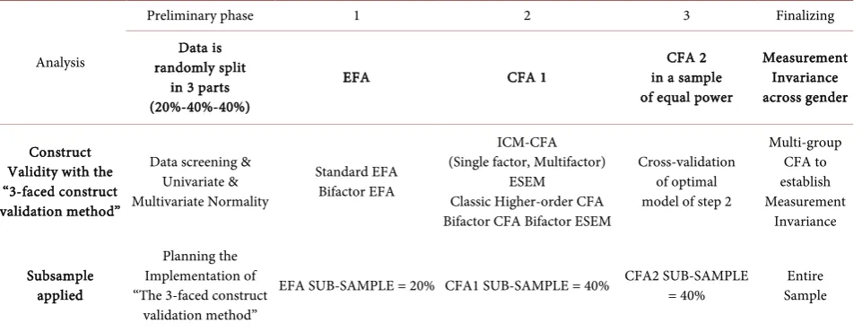
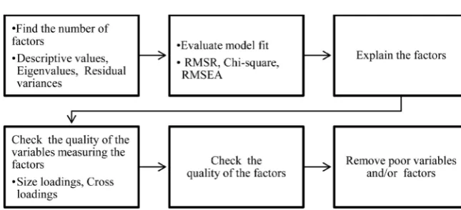
[image:5.595.61.542.515.700.2]During the process, multiple methods of exploratory and confirmatory factor analysis are used. In the EFA subsample, an Exploratory Factor Analysis and a Bifactor Exploratory Factor Analysis (Bifactor EFA) are carried out. In the CFA 1 subsample of 40%, CFA methods evaluated include an Independent Cluster Model Confirmatory Factor Analysis (ICM-CFA), a Bifactor Confirmatory Fac-tor Analysis (BifacFac-tor CFA), ExploraFac-tory Structural Equation Modeling (ESEM), and a Bifactor Exploratory Structural Equation Modeling (Bifactor ESEM) and a traditional higher-order CFA when applicable. Except for multiple methods, testing multiple alternative factor solutions for the instrument is generally con-sidered a good practice (Reise et al., 2007).
Table 1. Overview of the 3-faced construct validation method.
Analysis
Preliminary phase 1 2 3 Finalizing
Data is randomly split
in 3 parts (20%-40%-40%)
EFA CFA 1 in a sample CFA 2
of equal power
Measurement Invariance across gender
Construct Validity with the “3-faced construct validation method”
Data screening & Univariate & Multivariate Normality
Standard EFA Bifactor EFA
ICM-CFA (Single factor, Multifactor)
ESEM Classic Higher-order CFA Bifactor CFA Bifactor ESEM
Cross-validation of optimal model of step 2
Multi-group CFA to establish Measurement Invariance Subsample applied Planning the Implementation of “The 3-faced construct
validation method”
EFA SUB-SAMPLE = 20% CFA1 SUB-SAMPLE = 40% CFA2 SUB-SAMPLE = 40% Sample Entire
Note. EFA = Exploratory Factor Analysis, ICM-CFA= Independent Cluster Model Confirmatory Factor Analysis, ESEM = Exploratory Structural Equation Modeling.
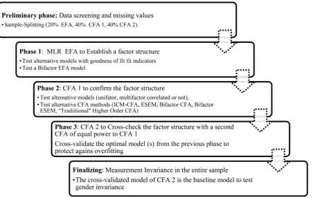
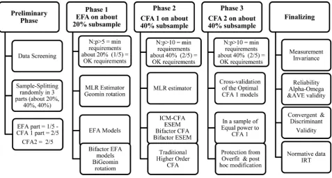
Next, the optimal CFA model that will emerge from the CFA 1 40% subsam-ple will be cross-validated in a different subsamsubsam-ple of equal power to that of CFA 1, i.e. 40%. In this phase, the optimal CFA structure is evaluated further on a different subsample. If alternative competing optimal models emerged, then they all be cross-checked. Then, a multi-group CFA (MGCFA) follows over the entire sample (20% + 40% + 40%) using the optimal model of the CFA 2 as a baseline model, to test for strict measurement invariance across gender. For the EFA phase the cases-per-variable threshold is set above 5:1, preferably above 10:1 (minimum requirements) to create an approximately 20% subsample or 1/5 (adequate conditions). In this 1/5 part of the sample EFA and Bifactor EFA models are evaluated. Then for the first CFA phase the minimum conditions are the cases-per-variable threshold to be above 10:1, preferably above 20:1 to create the adequate conditions for the 40% subsample (2/5) to emerge. In this phase al-ternative CFA models are examined, i.e., ICM-CFA, Bifactor CFA, ESEM and Bifactor ESEM models. For the second CFA phase the optimal model(s) is cross-validated by yet another CFA in a subsample of also 40%. That is an equal-power subsample of 2/5 to keep the minimum and required conditions the same to the ones of the first CFA. This phase is included as a protection against overfitting to safeguard the replicability of the optimal model deriving from the study (see the steps of the method in Table 1 and in Figure 1).
Preliminary Phase
[image:6.595.77.530.422.708.2]Generally, applied research (CFA or other) without missing values is consi-dered a luxury because missing data strategies, as a rule, mean loss of statistical
Figure 1. Description of the basic phases of the 3-faced construct validation method.
power, biased parameter estimates, standard errors, and test statistics (Allison, 2002, 2003; Enders, 2010; Little & Rubin, 2002; Schafer & Graham, 2002)as cited by Brown (2015). However, online digital test-batteries offer ways to overcome the problems inherent in missing data and they are freely available, like Google Forms, by Google®. One of them is to set the fields of the test battery as required
(See the successful implementation of this method in Kyriazos et al., 2018a,
2018b, 2018c). This can reduce or even eliminate the missing values problem (except longitudinal studies where respondents may be missing between
differ-ent research waves (seeBrown, 2015).
Data screening and sample size
Data screening is an equally important first step because CFA and Structural Equation Modeling, in general, are methods based on correlations, therefore the range of the data values, missing data, outliers, or non-linearity can influence the
results (Schumacker & Lomax, 2015). Outliers and influential cases may be
de-leted from the data (Muthen & Muthen, 2012). Additionally, sample size in
fac-tor analysis is a heavily debated issue because the replicability of a facfac-tor struc-ture is at some extend dependable on the sample size of the analysis and as a rule, a factor solution emerging from a large sample is potentially more reliable
than the one from a smaller sample (Devellis, 2017; MacCallum, Widaman,
Zhang, & Hong, 1999). A priori definition of the sample size is suggested to achieve the desired level of statistical power in a CFA or EFA with a given
in-strument (McQuitty, 2004; Brown, 2015; Singh et al., 2016; Tabachnick & Fidell,
2013).
A priori or not, both the relative (i.e., to the number of variables analyzed) and the absolute number of cases in the sample is suggested to be considered in
factor analysis (DeVellis, 2017; MacCallum et al., 1999) as well as additional
pa-rameters pertaining to SEM research in general like the study design (cross- sectional vs. longitudinal), model complexity, items reliability, response scale,
distribution and parameter estimator (Brown, 2015;Kline, 2016). Many rules of
thumb have been proposed about the minimum sample size requirements in factor analysis, e.g., N ≥ 50 (Pedhazur & Schmelkin, 1991), N ≥ 100 (Comrey & Lee, 1992), N ≥ 200 (Sivo et al., 2006; Garver & Menter, 1999; Hoelter, 1983; Hoe, 2008; MacCallum et al., 1999) or N ≥ 300 (Tabachnick & Fidell 2013).
Comrey and Lee (1992, 1973) offer the following guidelines to factor analysis sample size: 100 as poor, 200 as fair, 300 as good, 500 as very good, and 1000 or
more as excellent. Nevertheless, Kline (2016) reports a Monte Carlo study
(Clark, Miller et al., 2013) elaborating on the difficulty with a “one-size-fits-all” approach to sampling size in factor analysis.
Other suggestions include a minimum number of cases for each free model parameter or the “N:q rule” proposing at least 10 cases per free parameter, or the
“N:p rule” suggesting a minimum of 5 to 10 cases per model indicator (Bentler &
Chou, 1987; Ding, Velicer, & Harlow, 1995; Comrey & Lee, 1992; Gorsuch, 1983; Anderson & Gerbing, 1988; Hu, Bentler, & Kano, 1992), or even 20 cases
(Costello & Osborne, 2005; Schumacker & Lomax, 2015). However, as the
sam-ple gets larger, the ratio of cases per indicator can be lowered, therefore Tinsley
and Tinsley (1987) proposed a ratio of 5 to 10 cases per item for N ≥ 300 and a progressively lower ratio for larger sample sizes (DeVellis, 2017).
In brief, in the 3-faced construct validation method, a strategy to eliminate
missing data is to use the digital forms to collect data with the fields of the test battery set as required. Data is then suggested to be screened for outliers. Re-garding sample power, the “N:p rule” is used with a minimum of 5 cases per dicator in the model for the EFA, ideally 10:1 and a minimum of 10 cases per in-dicator in the model for CFA, ideally 20:1. Of course, more sophisticated
me-thods also exist to perform power analysis (McCall, 1982; Satorra & Saris 1985;
Jaccard, Jaccard, & Wan, 1996), including bootstrapping and Monte Carlo, but they are beyond the scope of this work. “Although the relationship of a sample size to the validity of factor analytic solutions is more complex than these rules of thumb indicate, they will probably serve investigators well in most
circums-tances”, as DeVellis (2017: p. 175)concludes.
Sample-Splitting
Sample splitting is generally used in cross-validate modeling in SEM and is
especially recommended for verifying a post hoc CFA model (Byrne, 2012;
Brown, 2015; Wang & Wang, 2012; Kline, 2015) or when testing a new
instru-ment (DeVellis, 2017). A general suggestion is to halve the sample when the size
is large enough to accommodate it (Byrne, 2012;Wang & Wang 2012) or to
di-vide it in two unequal parts when the size is smaller using the larger subsample for a calibration or construction sample and the second as validation sample
(DeVellis, 2017). One additional recommended method of sample splitting is
into one-third and two-thirds (Guadagnoli & Velicer 1988; MacCallum et al.
1996). Singh et al. (2016) abide by this method and they suggest an EFA be car-ried out in one-third data, and a CFA on two-thirds of the data as SEM requires
large samples (Kline, 2016). The factor structure emerges as they suggest form
the final list of domains and items (Singh et al., 2016).
In the 3-faced construct validation method, the sample is randomly split into
three subsamples, 20%, 40% and 40%. The first 20% subsample is used for an EFA, the second 40% subsample for a CFA and the third 40% subsample for an additional “twin” CFA, i.e. a CFA where the findings of the previous CFA are cross-checked in a sample of equal power. Caution is taken to keep the sample to model indicators ratio > 5 in the 20% EFA sample (minimum condition and adequate condition respectively) and >10 in the “twin” 40% CFA samples (>10 is again the minimum condition and 40% is the adequate condition). However, to end up inadequately powerful subsamples, the initial sample must be large enough and this is an issue addressed during the planning of the study. This is not feasible in special population studies and when studying certain the
con-structs, like flow (Csikszentmihalyi, 2000) that require special data collection
processes (e.g. ESM; Csikszentmihalyi, Larson, & Prescott, 1977).
Note that sample sizes in absolute numbers are only a rough guide, to indi-cated the logic pertaining the method, what is of greater importance when split-ting a sample is to maintain the N:p ratios above the threshold of 5:1 for EFA and 10:1 for CFA. However, what to keep in mind is not the exact percentage to split a sample. Instead, what to keep in mind is that when the cases to indicators ratios are at the specified levels the minimum conditions are met. Then the sam-ple can be divided into five parts and the adequate conditions will have been met too. One part can be used for the EFA and the four parts for the two CFAs (2 parts for each). This would result in a sample x for EFA and 2x for each CFA as SEM requires large samples.
Next, the assumption of normality is examined in all four samples emerging
after splitting, i.e. Total, EFA (20%), CFA 1 (40%), CFA 2 (40%), see Table 2.
The assumption of univariate normality is evaluated first using
Kolmogo-rov-Smirnov tests (Massey, 1951)on each of the indicators. Then, multivariate
normality is examined by the following four tests: 1) Mardia’s multivariate
kur-tosis test (Mardia, 1970); 2) Mardia’s multivariate skewness test (Mardia, 1970);
3) Henze-Zirkler’s consistent test (Henze & Zirkler, 1990), and 4)
Door-nik-Hansen omnibus test (Doornik & Hansen, 2008). A multivariate normal
distribution denotes that the univariate and bivariate normality assumption is
also not violated (Hayduk, 1987; Wang & Wang, 2012). See an overview of this
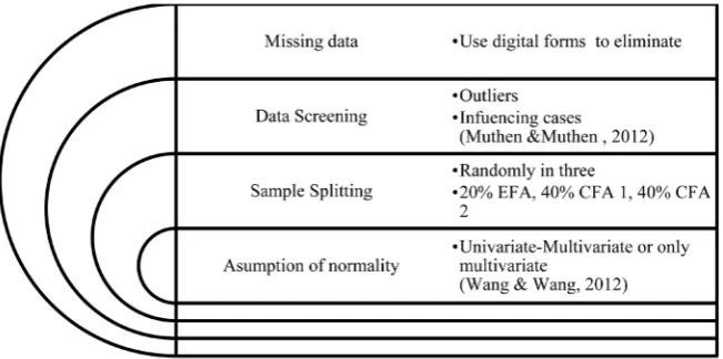
phase in Figure 2.
Phase 1: Establishing a factor structure with Exploratory Factor Analysis (EFA)
Exploratory factor Analysis (Spearman, 1904; Spearman, 1927) adopts the
premises of the common factor model (Thurstone, 1935, 1947). EFA is used to
explore the dimensionality of a measurement instrument (e.g. questionnaire or ability test) by defining a minimum set of factors required to interpret the corre-lations among a set of variables. It is exploratory because it only specifies the number of latent factors without defining an a priori structure on the linear
[image:9.595.212.538.532.694.2]rela-tionships between the observed variables and the latent factors (Muthén &
Figure 2. Description of the Preliminary Phase of the 3-faced construct validation me-thod.
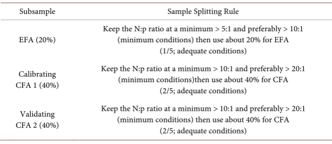
Table 2. Rules for splitting the sample in three pats in the 3-faced construct validation method.
Subsample Sample Splitting Rule
EFA (20%) Keep the N:p ratio at a minimum > 5:1 and preferably > 10:1 (minimum conditions) then use about 20% for EFA (1/5; adequate conditions)
Calibrating CFA 1 (40%)
Keep the N:p ratio at a minimum > 10:1 and preferably > 20:1 (minimum conditions)then use about 40% for CFA
(2/5; adequate conditions)
Validating CFA 2 (40%)
Keep the N:p ratio at a minimum > 10:1 and preferably > 20:1 (minimum conditions) then use about 40% for CFA
(2/5; adequate conditions)
Muthén, 2009a). This set of underlying variables discovered is the factor
solu-tion, which constitutes the construct being measured (Sawilowsky, 2007). Five
basic questions emerge during the EFA process: 1) Is the data suitable for factor analysis? 2) How will the factors be extracted? 3) What criteria will assist in de-termining factor extraction? 4) What rotational method will be used? 5) is the factor solution interpret table? (Williams et al., 2010). Therefore, it is considered an indeterminate solution because there are a plethora of available choices
mak-ing the method rather heuristic (Sawilowsky, 2007; Costello & Osborne, 2005;
Williams, Brown, & Onsman, 2010; Brown, 2015; Thompson, 2004; Tabachnick and Fidell, 2013). Note that in this work EFA is differentiated from Principal
Components Analysis (Costello & Osborne, 2005; Fabrigar & Wegener, 2012;
Brown, 2015 to name a few).
Conventionally, EFA is considered an exploratory method used in absence of a priori assumptions about factor structure and CFA methods are based on a
priori assumptions about the factor structure of a scale (Williams et al., 2010;
Fabrigar & Wegener, 2012; Kahn, 2006; Preacher, MacCallum et al., 2003; How-ard et al., 2016). The fundamental difference between EFA and CFA is that in the former all cross-loadings are freely estimated while in CFA (more precisely in the Independent Cluster Model CFA or ICM-CFA; see Morin et al., 2014) by default all cross-loadings are constrained to be zero. The free estimation of
cross-loadings renders EFA more explorative than CFA (Morin et al., 2013: p.
396; Howard et al., 2016). On the other hand, a presumed advantage of CFA in comparison to EFA is the specific goodness of fit criteria with the calculation of model fit indices.
Nonetheless, when EFA is carried out with estimators used also in CFA the same goodness of fit indicators can be calculated. Such estimators include the maximum likelihood parameter estimate (ML), or the Robust maximum
like-lihood estimation (MLR, Muthen & Muthen, 2012 or MLM; Bentler, 1995) that
are robust to non-normality. Additionally, MLR is appropriate for medium to small samples (Bentler & Yuan, 1999; Muthen & Asparouhov, 2002; Wang & Wang, 2012) like those emerging after sample-splitting. The MLR estimator is a
corrected normal theory method with robust standard errors and corrected
model test statistics (Wang & Wang, 2012; Savalei, 2014; Kline, 2016; Brown,
2015). Actually, MLR (or ML or MLM) EFA is considered as a special case of SEM (Brown, 2015). Like in CFA and SEM, in MLR EFA goodness-of-fit infor-mation is available to determine the appropriate number of factors (such as
chi-square and the root mean square error of approximation, or RMSEA; Steiger
& Lind, 1980).
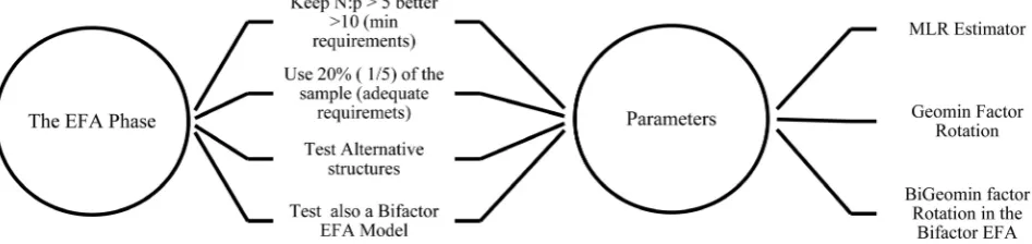
During the EFA phase of the of the 3-faced construct validation method, an
MLR EFA is carried out in the first 20% subsample taking into account the above-mentioned properties of MLR. The factor rotation used is the oblique
ro-tation of GEOMIN (see Muthen & Muthen, 2012). As a rule, an oblique rotation
is preferable in social sciences because it is considered a more realistic
represen-tation of factors interrelations. As Brown (2015) comments if the factors are
ac-tually uncorrelated, the oblique rotation will offer a model identical to the or-thogonal rotation model. On the other hand, if the factors are interrelated, an oblique rotation will offer a more accurate representation of the magnitude of the factor relationships along with important information like redundant factors or a potential higher-order structure. Moreover, when EFA is used in cohort with a subsequent CFA, like in this case, oblique solutions are more likely inter-pretable to CFA models than orthogonal solutions, because uncorrelated factors
tend to have poor model fit (Brown, 2015).
Additionally, MLR (or ML) EFA facilitates estimation of multiple models testing different numbers of factors to compare model fit, in tandem with other
criteria (Brown, 2015)like theoretical background of the solution, cross-loadings,
poorly defined factors and number of items per factor (Fabrigar et al. 1999;
Gorsuch 1983; Russell 2002; Fabrigar & Wegener, 2012; Costello & Osborne, 2005). Thus, multiple EFA models are generally tested in the MLR EFA
subsam-ple (20% of N with an N/p threshold of 5:1, preferably 10:1). MLR EFA is
per-formed to establish a factor structure (Porter & Fabrigar, 2007) testing
alterna-tive models with 1-3 or more factors. Second, an EFA Bifactor model (Jennrich
& Bentler, 2011) is tested subsequently when applicable (m > 1; Muthen & Mu-then, 2012). Reise et al. (2007) suggested that the evaluation of a Bifactor model
is a good practice when establishing construct dimensionality (c.f. Hammer &
Toland, 2016). See MLR EFA process in Figure 3.
Specifically, Bifactor analysis is a form of confirmatory factor analysis originally
introduced by Holzinger (1937). The bifactor model has a general factor and a
set of specific factors (Brown, 2015). An advantage of EFA bi-factor analysis is that an a priori model is not necessary. The results of an EFA bifactor analysis, however,
can be used as a basis for defining a CFA Bifactor model (Howard et al., 2016).
The EFA Bifactor factor analysis (Jennrich & Bentler, 2011, 2012) in the 3-faced construct validation method is carried out using also MLR to estimate model
parameters and a BI-GEOMIN factor rotation (Jennrich & Bentler, 2011, 2012),
as a rule. The BI-GEOMIN is an oblique rotation where the specific factors are
Figure 3. MLR EFA Steps as described by Muthén & Muthén (2009b).
correlated with both the general factor and with each other. If the orthogonal rotation is used, then the specific factors are uncorrelated both with the general
factor and with each other (Muthen & Muthen, 2012). However, a word of
cau-tion is required because Bifactor models always tend to support unidimensional-ity (Joshanloo, Jose, & Kielpikowski, 2017) and higher order factor structure
based only on a Bifactor model is often regarded questionable (Joshanloo &
Jo-vanovic, 2017).
MLR EFA model fit is evaluated by the following criteria (Hu & Bentler, 1999;
Brown, 2015): RMSEA (≤.06, 90% CI ≤ .06), SRMR (≤.08), CFI (≥.95), TLI
(≥.95), and the chi-square/df ratio less than 3 (Kline, 2016). See the EFA phase in
Figure 4.
Like already said, EFA is an exploratory process, therefore, EFA results are
generally with additional CFAs on a different data set (Cudeck, MacCallum et
al., 2007; Bollen, 2002; Brown, 2015; Schumacker & Lomax, 2015). CFA is the
subsequent phase of the 3-faced construct validation method.
Phase 2: Confirming the factor structure with Confirmatory Factor Anal-ysis (CFA)
CFA is integrated into the Structural Equation Modeling (SEM) framework. SEM comprises models in which regressions among continuous latent variables are estimated (Bollen, 1989; Browne & Arminger, 1995; Joreskog, Sorbom, & Magidson, 1979; Muthen & Muthen, 2012). Thus a CFA model construction fol-lows the same steps as an SEM model: 1) Model specification. Theory and prior research play an important role in a CFA model specification because it is based on previous research and knowledge. 2) Model identification. In CFA a model is
identified by constraining some parameters and freely estimating others. 3)
Model estimation. Estimating the fit of the free parameters of the specified factor model. 4) Testing model fit 5) Model modification. Changes to a specified model
are considered when the specified model is less than satisfactory (Kelloway,
2015; Schumacker & Lomax, 2015).
During this phase of the 3-faced construct validation method the factor
struc-ture established in the MLR EFA subsample (20% of N with a N:p threshold of
5:1, preferably 10:1) it is confirmed with an CFA (40% of N with a N:p threshold
Figure 4. Description of the EFA Phase of the 3-faced construct validation method.
of 10:1, preferably 20:1). This is accomplished by testing alternative models with
multiple CFA methods. CFA methods used in the 3-faced construct validation
method are the following: 1) Independent Cluster Model Confirmatory Factor Analysis (ICM-CFA), 2) Exploratory Structural Equation Modeling Analysis (ESEM), 3) Bifactor Confirmatory Factor Analysis (Bifactor CFA), and 4) Bifac-tor ExploraBifac-tory Structural Equation Modeling Analysis (BifacBifac-tor ESEM), 5) Higher order CFA (when applicable).
In ICM-CFA is the basic Independent Clusters Model of Confirmatory Factor Analysis that posits all items have zero factor loadings on all other factors except
the one they are intended to measure (McDonald, 1985; Morin et al., 2016;
Howard et al., 2016). Even trivial cross-loadings when constrained to be zero
results in inflated CFA factor correlations (Asparouhov & Muthén, 2009; Marsh
et al. 2009, 2010). ESEM (Asparouhov & Muthén, 2009) is an integration of CFA and EFA. In EFA all cross-loadings are freely estimated and in ESEM a specific
percentage of cross-loadings are allowed to be freely estimated (Muthen &
Mi-then, 2012). This potentially resolves the factor inflation problem inherent in ICM-CFA, especially pertinent in psychology research where constructs
gener-ally tend to be correlated (Marsh, Morin, Parker & Kaur, 2014). As a rule, ESEM
potentially produces more accurate models in comparison to ICM-CFA (How-ard, Gagne, Morin, Wang & Forest, 2016). Therefore, testing ESEM models
(when m > 1) is generally regarded as a good practice when testing
dimensional-ity of an instrument.
In the3-faced construct validation method the CFA methods is suggested to
test the higher order factor structure are the following: 1) Bifactor Models:
Bi-factor CFA, BiBi-factor ESEM; and 2) Second-order CFA. BiBi-factor analysis
(Har-man, 1976; Holzinger & Swineford, 1937) is another approach to higher-order factor analysis, specifying direct effects of the higher-order dimension (General factor) on the indicators (Specific factors), unlike the classical higher-order CFA method. The benefit of the exploratory Bifactor analysis method is that a specific
a priori bi-factor model is not necessary. In Bifactor ESEM (c.f. Reise, 2012;
Marsh et al., 2014) direct effects of the higher-order dimension are specified and
additionally because ESEM (Asparouhov & Muthén, 2009) can potentially
re-solve misspecifications and inflated factor loadings, inherent in CFA method as
a result of forcing secondary factor loadings to be equal to zero (Marsh et al.,
2014). Concerning the theoretical construct behind the Bifactor higher order structure, bifactor models are most appropriate for unidimensional constructs,
having at the same time smaller latent sub-factors (Brown, 2015). Actually, Reise
et al. (2007) recommended testing a bifactor model when examining dimension-ality. The traditional higher order factor analysis is typically carried out because occasionally first-order factors indicate narrow-scope constructs, interconnected with a higher and broader construct represented in factor analysis by one or
more higher order factors (Cattell, 1978; Comrey, 1988; Gorsuch, 1983 cited in
Wolff & Preising, 2005). Thus, higher-order CFA (most of the times second-order) is a theory-based solution with an additional, more parsimonious higher structure that represents the latent factor interrelationships established in
the CFA (Brown, 2015; Wang & Wang, 2012).
Alternative models evaluated in the 3-faced construct validation method are
the following: 1) a Unidimensional model to test the assumption of maximum
parsimony (Brown, 2015; Crawford & Henry, 2004); 2) Uncorrelated factors
model; or/and 3) Correlated factors model(s) based on theory and previous
em-pirical research (Schumacker & Lomax, 2015); 4) Second-order factor models
are tested if possible. Specifically, when first-order factors > 3, evaluating if the second-order factor improves the model fit when compared to the first-order solution is not possible because of under-identification of the higher order
model (Wang & Wang, 2012); and 5) Bifactor models (CFA and ESEM) are
tested if applicable, i.e. if m > 1 (Muthen & Muthen, 2012), suggested by Reise et al. (2007)to be a good practice (also by Hammer & Tolland, 2016). See all CFA 1 methods tested in Table 3.
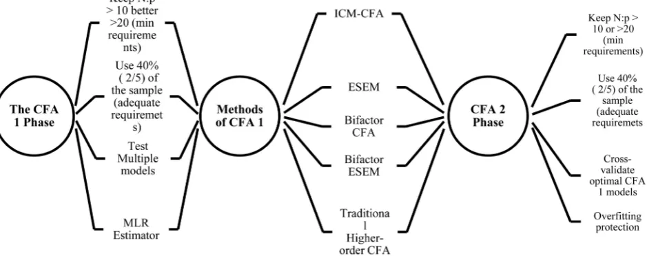
Regarding model parametrization (see also Figure 5) in the 3-faced construct
validation method MLR is generally suggested as a parameter estimator for all CFA models evaluated, like in EFA for reason. Model fit is estimated by the
fol-lowing criteria (Hu & Bentler, 1999; Brown, 2015): RMSEA (≤.06, 90% CI ≤ .06),
SRMR (≤.08), CFI (≥.95), TLI (≥.95), and the chi-square/df ratio less than 3
(Kline, 2016). There are abundant indicators of goodness-of-fit, both absolute
and incremental (Singh et al., 2016), and researchers are generally urged
eva-luating model fit by taking into consideration multiple fit indicators to have
more conservative model fit estimation (Bentler & Wu, 2002; Hair et al., 2010;
Brown, 2015; Kline, 2016). A second CFA in a sample of equal power to the first
[image:14.595.212.530.629.701.2]CFA is the next phase of the 3-faced construct validation method.
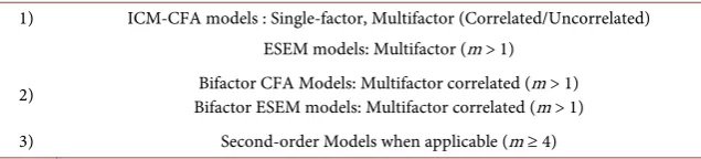
Table 3. CFA methods included in the 3-faced construct validation method and models tested per method.
1) ICM-CFA models : Single-factor, Multifactor (Correlated/Uncorrelated) ESEM models: Multifactor (m > 1)
2) Bifactor ESEM models: Multifactor correlated (m > 1) Bifactor CFA Models: Multifactor correlated (m > 1)
3) Second-order Models when applicable (m ≥ 4)
Note. m = number of latent variables, EFA = Exploratory Factor Analysis, ICM-CFA = Independent Clus-ter Model Confirmatory Factor Analysis, ESEM = Exploratory Structural Equation Modeling.
Figure 5. Description of the CFA 1 Phase and CFA2 Phase of the 3-faced construct validation method.
Phase 3: Cross-checking the factor structure with a second Confirmatory Factor Analysis (CFA)
In the realm of SEM, the cross-validation method of testing replicability (see
the section “Why need a Method?”) is called cross-validation modeling (Wang &
Wang, 2012). A cross-validation CFA is the 3rd phase of the 3-faced construct va-lidation method (see Figure 5). During this phase the optimal model(s)
emerg-ing from the initial CFA of the previous phase (implemented on 40% of N with a
N:p threshold of 10:1, preferably 20:1) are replicated on a new subsample that
has the same sample power to the initial CFA subsample, i.e. in the 40% of N
with a N:p threshold of 10:1, preferably 20:1). Cross-validation is a persuasive strategy for addressing the implications of post hoc modeling and the potential over-optimization inherently connected with post hoc model modification but also partial invariance (Byrne, 2012; Wang & Wang 2012).
In this phase, the optimal models emerging from this phase are compared to each other. An additional model comparison is carried out using the following guidelines: 1) a likelihood ratio test, 2) information criteria and 3) modification indices. The models are considered superior they have: 1) a lower Akaike Infor-mation Criterion (AIC), 2) a lower Bayesian inforInfor-mation criterion (BIC) 3) If models significantly differ, the more complicated model is preferable, 4e) If models do not significantly differ, the less complicated model is preferable
(Epskamp et al., 2017). To compare the fit of the optimal solutions with alterna-tive choices to the ML estimator for non-normal data (like MLR) the MLR res-caled version of the “likelihood ratio test” (2ΔLL; Satorra & Bentler, 2010) is calculated and if it is statistically significant, the equal factor variance hypothesis can be rejected (Wang & Wang, 2012). This essentially suggests that there is a fit difference between the optimal CFA models.
It is generally suggested by the 3-faced construct validation method to
cross-validate a group of optimal models with the comparable goodness of fit
and not just the best fitting solution because often a local optimum fitting model emerges, showing a divergence in fit during the two CFAs. Additionally, this is a protection against over-fitting due to post hoc model revision to achieve a better fit that most often is not replicable in the validation subsample. Overfitting— specifying unnecessary parameters to the model to improve fit—is generally re-garded as a consequence of non-theory-driven specification searches daring
model modification and capitalization on chance (Brown, 2015). This means
that weak effects in the data-set are targeted emerging mainly from sampling
er-ror, thus are non-replicable in a different data-set(MacCallum, Roznowski, &
Necowitz, 1992; MacCallum, 1986; Silvia & MacCallum, 1988; Byrne, 2012; Kline, 2016; Brown, 2015). Cross-validating a post-hoc model in a new subsample generally suggests that the likelihood of non-replicability is lower in comparison to a non-cross-validated sample but not minimal. In other words, cross-validation is a necessary but insufficient requirement to protect against non-replicability
due to sample idiosyncrasies (Karson, 2007). Additionally, there is always the
chance a good fitting model to be non-replicable in the second sample. Then the researcher should choose a different model that is more stable across all three subsamples (EFA, 20%, CFA 1 40% and CFA 2 40%) and not necessarily the
model of the best fit. There are some examples for applying this method
(Kyria-zos et al., 2018a, 2018b, 2018c, 2018d) where such a case emerged (Kyriazos et al, 2018e).
Generally, the post hoc model fitting has been heavily debated in SEM and
CFA literature regarding Type I errors (Byrne, 2012; Brown, 2015) and it is a
strategy mainly recommended for minimizing implications resulting from post
hoc model fitting (Wang & Wang, 2012). It is generally suggested that the final
model of a post hoc analysis to be tested on a second (or more) independent
sample(s) from the same population (see also Byrne, 2012; Byrne, 2006). Several
other approaches were also proposed as a remedy (e.g. Green & Babyak, 1997;
Green, Thompson, & Poirier, 2001; Chou & Bentler, 1990; Green, Thompson, & Poirier, 1999) as Byrne (2012) reviews. The last remedy to the problem of chance
factors—as Byrne (2012) continues—is to cross-validate the final post hoc
mod-ified model in a different sample either new or subsample with sample-splitting
(see also Thompson, 2000 and MacCallum and Austin, 2000).
Byrne et al. (1989), as reported by Wang & Wang (2012), also raised certain practical issues regarding cross-validation. The most important of them is the accessibility to a sufficiently large sample to be split, and the possibility of failure of the cross-validation when multiple parameters are relaxed in the first sample
(Wang & Wang 2012). Some other experts also questioned the method (Cliff, 1983; Cudeck & Browne, 1983) while others (Byrne et al., 1989, Byrne, 2012, Byrne, 2006) suggest that as long as the researcher keeps in mind the exploratory nature of the CFA cross-validation analysis, the cross-validation process is useful
(Byrne, 2011; MacCallum, Roznowski, Mar, & Reith, 1994; MacCallum, We-gener, Uchino, & Fabrigar, 1993). Above all, CFA researchers are aware of the
exploratory nature of the post hoc procedures if not theoretically substantiated
(Byrne, 2012).
Finalizing: Measurement invariance of the cross-validated optimal CFA model
In the final phase of the 3-faced construct validation method measurement
invariance of the instrument is examined across gender in the entire sample
(100% of N). Generally, measurement invariance examines if an instrument
ex-hibits the same psychometric properties across heterogeneous groups (Chen,
2007) or across time (Brown, 2015). When doing multiple-group confirmatory
factor analysis, this assumption can be tested directly (Timmons, 2010).
To test for measurement invariance across gender groups in the 3-faced
con-struct validation method the optimal model, successfully cross-validated in the second CFA, is used as a baseline model. First, gender invariance of the success-fully cross-validated model is tested separately in each gender group, to establish a baseline model. This model should show an equally good fit for both gender groups. Then, this baseline solution is tested in both gender groups
simulta-neously and if the fit is adequate configural invariance is supported (Horn,
McArdle, & Mason, 1983). The chi-square, RMSEA, CFI, and other fit indexes are used to determine whether the combined model has a good model fit to support configural invariance. Next, factor loadings, indicator intercepts, and indicator residuals are consecutively constrained to equality. The ΔCFI and ΔRMSEA for the constrained models are evaluated to indicate weak, strong and
strict invariance respectively the ultimate test of measurement invariance (Wang
& Wang, 2012). The criteria used are the ΔCFI ≤ −.01, and ΔRMSEA ≤ .015 for N > 300 (Chen, 2007: p. 501). Suggested criteria in the literature are also defined by Cheung & Rensvold (2002).
Alternatively, if the sample is not sufficient (e.g. N = 150) measurement
riance can be omitted and population heterogeneity and measurement inva-riance can be evaluated for latent means and item intercepts with the Multiple Indicators Multiple Causes method (MIMIC) controlling for the effects of gend-er or age. Multiple Indicators Multiple Causes Modeling (MIMIC) or CFA with covariates is an alternative method for examining invariance of indicators and latent means in multiple groups, by regressing them onto covariates indicating
group membership (Muthén & Muthén, 2009a). Crucially, MIMIC models are
more appropriate for small samples (even of N = 150) than multiple-group CFA
(Brown, 2015: pp. 273-274). Initially, a viable measurement model is necessary, collapsing across specified groups (i.e., a typical CFA model). For this purpose, in the 3-faced construct validation method the optimal model that was
success-fully cross-validated in the second CFA is used in the full sample (100% of N).
Then, as a rule, the covariates of gender and age are added to examine their di-rect effects on the factor(s) and selected indicators of the model, i.e. the regres-sion of a factor indicator on a covariate in order to study population
heterogene-ity and measurement non-invariance respectively (Muthen & Muthen, 2012;
Brown, 2015). Unlike multiple-groups CFA, MIMIC models test only if there is
invariance in the indicator intercepts and factor means, assuming that all other measurements and structural levels of invariance (i.e., equal factor loadings, er-ror variances/covariances, factor variances/covariances) are supported same across covariates (Brown, 2015).
Remember that to establish measurement invariance in the 3-faced construct
validation method the optimal model that was successfully cross-checked in the second CFA (40% of the sample) is tested over the entire sample to become a baseline model, thus, in essence, this is yet another cross-validation of the op-timal model emerged from the whole process. Note also that measurement inva-riance can be evaluated in higher levels, like vainva-riance and covainva-riance invainva-riance
(Widaman & Reise, 1997). However, configural, factor loading, indicator inter-cepts, and indicator residuals invariance are the most invariance tests carried out in the majority of the studies (Chen, 2007).
4. Method Summary and Applicability
To establish the construct validity of an instrument designed for a different cul-tural context we developed a multiphase cross-validation procedure called the “3-faced construct validation method” (see method phases in Figure 6). Note that this method does not cover the translation phase but the subsequent stages.
The method is based on sample-splitting. Sample-splitting (Guadagnoli &
Velic-er, 1988; MacCallum, Browne, & Sugawara, 1996) is generally regarded as a cross-validation method because factor analysis findings are replicated in a
dif-ferent subsample (Byrne, 2012;Brown, 2015; Schumacker & Lomax, 2015; Singh
[image:18.595.62.540.451.707.2]et al., 2016; DeVellis, 2017). In the “3-faced construct validation method” the
Figure 6. The 3-faced construct validation method.
sample is randomly split into three parts (20%, 40%, and 40%) keeping the N:p ratio threshold for the EFA to 5:1, preferably 10:1 and for CFA to 10:1, preferably 20:1. The first 20% is used for MLR EFA. Multiple structures are tested along with a Bifactor EFA model. Regarding sample power, in all three samples cau-tion is needed to be far beyond the suggested threshold of 5 to10 cases for each
observed variable (Singh et al., 2016) and even the stricter 20 cases for each
ob-served variable (Schumacker & Lomax, 2015).
The second 40% is used for an explorative CFA (CFA 1) to test a minimum of the following alternative models: a single-factor ICM-CFA, a multifactor ICM-CFA with correlated and uncorrelated factors and their ESEM counter-parts. Other theory-driven models to be tested include a Bifactor CFA model, a Bifactor ESEM model and a Higher-order CFA (if applicable). Next, the third 40% is used for a crosscheck CFA (CFA 2). This second CFA is intended to veri-fy the optimal model (or competing optimal models) emerged in the CFA 1 in a different subsample of equal power to the CFA 1 subsample (both 40%). If the CFA 2 fails to revalidate the optimal CFA 1 model, then the second best model is crosschecked etc. Measurement invariance using the cross-validated model as a baseline model is the final phase of the method. Note that, actually, the lesson to take home is not the exact percentages to split a sample but if the cases to indi-cators ratios are above the specified levels these are the minimum conditions to carry out the method. Thus, the sample can be divided into five parts and these are the adequate conditions to carry out the method. One part can be used for the EFA and the four parts for the two CFAs (2 parts for each). This would result in a sample x for EFA and 2x for each CFA as SEM requires large samples. If the sample is not adequate to be split in three and the structure of the validated in-strument is known then the sample can be halved to carry out two CFAs as a protection against overfitting. However, the rules setting the minimum and adequate conditions must be followed. For an unknown structure EFA must be carried out in the first halve and a CFA must follow in the second halve, however in this case the solution is not protected against ovefitting. The study of a known structure must be designed in a way that at least two CFAs can be carried out af-ter halving the sample.
The validation procedure is also suggested to include the following, in line with the general empirical method adopted for evaluating the psychometric properties of measurement instruments: 1) Reliability analysis using Cronbach’s alpha, Omega Total coefficient and AVE-based construct validity, 2) Correlation Analysis to Examine Convergent and Discriminant Validity, 3) Normative Data, 4) Item response theory (IRT). The entire sample is suggested to be used for the above analyses, but alpha could be also calculated for the subsamples too if de-sired (DeVellis, 2017).
More specifically, reliability and validity are evaluated in the entire sample
using the following measures; 1) Cronbach’s alpha (α; Cronbach, 1951) to
ex-amine internal consistency of the responses. Alpha values above .70 are generally acceptable (Hair et al., 2010), and above .80 adequate (Kline, 2000; Nunnally &
Berstein, 1994); 2) Omega Total coefficient (ω total; McDonald, 1999; Werts, Linn, & Jöreskog, 1974). Omega corresponds either to variance accounted by all
factors or by each latent factor separately (Brunner et al., 2012). For omega a,
value of .70 or greater is acceptable (Hair et al., 2010); 3) Average Variance
Ex-tracted (AVE; Fornell & Larcker, 1981) to evaluate convergent validity. Malhotra & Dash (2011) comment that ω alone is weak, potentially allowing an error va-riance as high as 50%. Therefore, AVE in combination with ω coefficient offers a
more conservative estimation of convergent validity (Malhotra & Dash, 2011).
The threshold for AVE is .50 (Fornell & Larcker, 1981; Hair et al., 2010). Regarding normative data, it is included along with the means and ranges of the instrument dimensions. Means are not informative of individual scores,
given the non-normality of the data (Crawford & Henry, 2004). Therefore,
scores are converted to percentiles. Finally, Item response theory (IRT) is carried out during the construction, analysis, scoring, and comparison of measurement instruments (questionnaires or ability tests) intended to measure an unobserva-ble characteristics of the respondents (Binary response models: 1PL, 2PL, 3PL; Categorical response models: GRM, NRM, PCM, RSM; Multiple IRT models combined: Hybrid).
5. Conclusion
In conclusion, the “3-faced construct validation method” is a routine indented
for establishing the validity and reliability of an existing scale when it is adapted in a different cultural context (not including the translation part). However, the routine can also be used for the initial validation of a newly developed instru-ment or for testing the measureinstru-ment model in a SEM study. Empirical
applica-tions of the method were carried out by Kyriazos et al. (2018a, 2018b, 2018c,
2018d, 2018e).
Sample-splitting (Guadagnoli & Velicer, 1988; MacCallum, Browne &
Suga-wara, 1996) is generally an acknowledged cross-validation method (Byrne, 2012; Brown, 2015). Similar approaches to the “3-faced construct validation method”
were also proposed by Brown (2015), by Singh et al. (2016), and by Muthén &
Muthén (2009a). Cross-validation is also used in SEM measurement models (see
Byrne, 2012) or in logistic regression to cross-validate the results (Lomax & Hahs-Vaughn, 2013).
The addition of the “3-faced construct validation method” in the empirical
research of psychometrics regarding the adaption of measurement instruments in a different cultural context than the one they were initially developed is: 1) The rule of keeping the MLR EFA and Bifactor EFA N:p ratio above a minimum of 5 cases per variable and preferably 10 using 20% of the sample 2) The use of the rest 80% of the sample to carry out two “twin” CFAs, i.e. two CFAs in two
subsamples of equal power 40% each(minimum requirements and adequate
re-quirements respectively). The rule here is to keep the CFA N: p ratio above a minimum of 10 cases per variable and preferably 20 using 40% of the sample for
each CFA. 3) The use of multiple methods in the first exploratory CFA and mul-tiple models (ICM-CFA, ESEM, Bifactor CFA, Bifactor ESEM, and “traditional” Higher-order CFA when applicable. What to keep in mind is not the exact per-centage to split a sample. Again it should be emphasized that the central message conveyed is if the cases to indicators ratios are above at the specified levels (minimum conditions) then the sample can be divided into five parts (adequate conditions). One part can be used for the EFA and the four parts for the two CFAs (2 parts for each). This would result in a sample x for EFA and 2x for each CFA as SEM requires large samples. The method is a protection against overfit-ting but it requires careful planning and a large sample.
Conflicts of Interest
The authors declare no conflicts of interest regarding the publication of this paper.
References
Allison, P. D. (2002). Missing Data. Thousand Oaks, CA: Sage. https://doi.org/10.4135/9781412985079
Allison, P. D. (2003). Missing Data Techniques for Structural Equation Modeling. Journal of Abnormal Psychology, 112, 545-557. https://doi.org/10.1037/0021-843X.112.4.545 Anderson, J. C., & Gerbing, D. W. (1988). Structural Equation Modeling in Practice: A
Review and Recommended Two-Step Approach. Psychological Bulletin, 103, 411-423. https://doi.org/10.1037/0033-2909.103.3.411
Asparouhov, T., & Muthén, B. (2009). Exploratory Structural Equation Modeling. Struc-tural Equation Modeling, 16, 397-438. https://doi.org/10.1080/10705510903008204 Bentler, P. M. (1995). EQS Structural Equations Program Manual. Encino, CA:
Multiva-riate Software.
Bentler, P. M., & Chou, C. P. (1987). Practical Issues in Structural Modeling. Sociological Methods & Research, 16, 78-117. https://doi.org/10.1177/0049124187016001004 Bentler, P. M., & Wu, E. J. C. (2002). EQS 6 for Windows Guide. Encino, CA:
Multiva-riate Software.
Bentler, P. M., & Yuan, K. H. (1999). Structural Equation Modeling with Small Samples: Test Statistics. Multivariate Behavioral Research, 34, 181-197.
https://doi.org/10.1207/S15327906Mb340203
Bollen, K. A. (1989). A New Incremental Fit Index for General Structural Equation Mod-els. Sociological Methods & Research, 17, 303-316.
https://doi.org/10.1177/0049124189017003004
Bollen, K. A. (2002). Latent Variables in Psychology and the Social Sciences. Annual Re-view of Psychology, 53, 605-634.
https://doi.org/10.1146/annurev.psych.53.100901.135239
Brown, T. A. (2015). Confirmatory Factor Analysis for Applied Research (2nd ed.). New York: Guilford Publications.
Browne, M. W., & Arminger, G. (1995). Specification and Estimation of Mean- and Co-variance-Structure Models. In Handbook of Statistical Modeling for the Social and Be-havioral Sciences (pp. 185-249). Boston, MA: Springer.
https://doi.org/10.1007/978-1-4899-1292-3_4
Brunner, M., Nagy, G., & Wilhelm, O. (2012). A Tutorial on Hierarchically Structured Constructs. Journal of Personality, 80, 796-846.
https://doi.org/10.1111/j.1467-6494.2011.00749.x
Byrne, B. M. (2006). Structural Equation Modeling with EQS: Basic Concepts,
Applica-tions, and Programming (2nd ed.). Mahwah, NJ: Lawrence Erlbaum Associates, Inc.
Byrne, B. M. (2012). Structural Equation Modeling with Mplus: Basic Concepts,
Applica-tions, and Programming. London: Routledge.
Byrne, B. M., Shavelson, R., & Muthen, B. (1989) Testing for the Equivalence of Factor Covariance and Mean Structures: The Issue of Partial Measurement Invariance. Psy-chological Bulletin, 105, 456-466. https://doi.org/10.1037/0033-2909.105.3.456
Cattell, R. B. (1978). Scientific Use of Factor Analysis in Behavioral and Life Sciences. New York: Plenum Press. https://doi.org/10.1007/978-1-4684-2262-7
Chen, F. F. (2007). Sensitivity of Goodness of Fit Indexes to Lack of Measurement Inva-riance. Structural Equation Modeling, 14, 464-504.
https://doi.org/10.1080/10705510701301834
Cheung, G. W., & Rensvold, R. B. (2002). Evaluating Goodness-of-Fit Indexes for Testing Measurement Invariance. Structural Equation Modeling, 9, 233-255.
https://doi.org/10.1207/S15328007SEM0902_5
Chou, C. P., & Bentler, P. M. (1990). Model Modification in Covariance Structure Mod-eling: A Comparison among Likelihood Ratio, Lagrange Multiplier, and Wald Tests. Multivariate Behavioral Research, 25, 115-136.
https://doi.org/10.1207/s15327906mbr2501_13
Clark, S. L., Miller, M. W., Wolf, E. J., & Harrington, K. M. (2013). Sample Size Require-ments for Structural Equation Models: An Evaluation of Power, Bias, and Solution Propriety. Educational and Psychological Measurement, 73, 913-934.
Cliff, N. (1983). Some Cautions Concerning the Application of Causal Modeling Me-thods. Multivariate Behavioral Research, 18, 115-126.
https://doi.org/10.1207/s15327906mbr1801_7
Comrey, A. L. (1988). Factor-Analytic Methods of Scale Development in Personality and Clinical Psychology. Journal of Consulting and Clinical Psychology, 56, 754.
https://doi.org/10.1037/0022-006X.56.5.754
Comrey, A. L., & Lee, H. B. (1973). A First Course in Factor Analysis. New York, NY: Academic Press.
Comrey, A. L., & Lee, H. B. (1992). A First Course in Factor Analysis. Hillsdale, NJ: Law-rence Eribaum Associates.
Comrey, A. L., & Lee, H. B. (1992). Interpretation and Application of Factor Analytic Results. In A. L. Comrey, & H. B. Lee (Eds.), A First Course in Factor Analysis (p. 2). Hillsdale, NJ: Lawrence Eribaum Associates.
Costello, A. B., & Osborne, J. W. (2005). Best Practices in Exploratory Factor Analysis: Four Recommendations for Getting the Most from Your Analysis. Practical Assess-ment, Research & Evaluation, 10, 1-9.
Crawford, J. R., & Henry, J. D. (2004). The Positive and Negative Affect Schedule (PANAS): Construct Validity, Measurement Properties and Normative Data in a Large Non-Clinical Sample. British Journal of Clinical Psychology, 43, 245-265.
https://doi.org/10.1348/0144665031752934
Crocker, L., & Algina, J. (1986). Introduction to Classical and Modern Test Theory. New York, NY: Holt, Rinehart and Winston.
Cronbach, L. J. (1951). Coefficient Alpha and the Internal Structure of Tests. Psychome-trika, 16, 297-334.https://doi.org/10.1007/BF02310555
Cronbach, L. J., & Meehl, P. E. (1955). Construct Validity in Psychological Tests. Psycho-logical Bulletin, 52, 281-302.https://doi.org/10.1037/h0040957
Csikszentmihalyi, M. (2000). Happiness, Flow, and Economic Equality.
Csikszentmihalyi, M., Larson, R., & Prescott, S. (1977). The Ecology of Adolescent Activ-ity and Experience. Journal of Youth and Adolescence, 6, 281-294.
https://doi.org/10.1007/BF02138940
Cudeck, R., & Browne, M. W. (1983). Cross-Validation of Covariance Structures. Multi-variate Behavioral Research, 18, 147-167.https://doi.org/10.1207/s15327906mbr1802_2 Cudeck, R., MacCallum, R. C., Millsap, R. E., & Meredith, W. (2007). Factor Analysis at
100: Historical Developments and Future Directions.
DeVellis, R. F. (2017). Scale Development: Theory and Applications (4th ed.). Thousand Oaks, CA: Sage.
Ding, L., Velicer, W. F., & Harlow, L. L. (1995). Effects of Estimation Methods, Number of Indicators per Factor, and Improper Solutions on Structural Equation Modeling Fit Indices. Structural Equation Modeling: A Multidisciplinary Journal, 2, 119-143.
https://doi.org/10.1080/10705519509540000
Doornik, J. A., & Hansen, H. (2008). An Omnibus Test for Univariate and Multivariate Normality. Oxford Bulletin of Economics and Statistics, 70, 927-939.
https://doi.org/10.1111/j.1468-0084.2008.00537.x
Enders, C. K. (2010). Applied Missing Data Analysis. New York, NY: Guilford Press. Epskamp, S., Rhemtulla, M., & Borsboom, D. (2017). Generalized Network Pschometrics:
Combining Network and Latent Variable Models. Psychometrika, 82, 904-927.
https://doi.org/10.1007/s11336-017-9557-x
Fabrigar, L. R., & Wegener, D. T. (2012). Exploratory Factor Analysis. New York, NY: Oxford University Press, Inc.
Fabrigar, L. R., Wegener, D. T., MacCallum, R. C., & Strahan, E. J. (1999). Evaluating the Use of Exploratory Factor Analysis in Psychological Research. Psychological Methods, 4, 272-299.https://doi.org/10.1037/1082-989X.4.3.272
Fornell, C., & Larcker, D. F. (1981). Structural Equation Models with Unobservable Va-riables and Measurement Error: Algebra and Statistics. Journal of Marketing Research, 382-388.https://doi.org/10.2307/3150980
Garver, M. S., & Mentzer, J. T. (1999). Logistics Research Methods: Employing Structural Equation Modeling to Test for Construct Validity. Journal of Business Logistics, 20, 33-57.
Gorsuch, R. L. (1983). Factor Analysis (2nd ed.). Hillsdale, NJ: LEA.
Green, S. B., & Babyak, M. A. (1997). Control of Type I Errors with Multiple Tests of Constraints in Structural Equation Modeling. Multivariate Behavioral Research, 32, 39-51.https://doi.org/10.1207/s15327906mbr3201_2
Green, S. B., Thompson, M. S., & Poirier, J. (1999). Exploratory Analyses to Improve Model Fit: Errors Due to Misspecification and a Strategy to Reduce Their Occurrence. Structural Equation Modeling: A Multidisciplinary Journal, 6, 113-126.
https://doi.org/10.1080/10705519909540122
Green, S. B., Thompson, M. S., & Poirier, J. (2001). An Adjusted Bonferroni Method for Elimination of Parameters in Specification Addition Searches. Structural Equation Modeling, 8, 18-39.
Guadagnoli, E., & Velicer, W. F. (1988). Relation of Sample Size to the Stability of Com-ponent Patterns. Psychological Bulletin, 103, 265-275.
https://doi.org/10.1037/0033-2909.103.2.265
Hair, J., Black, W., Babin, B., & Anderson, R. (2010). Multivariate Data Analysis (7th ed.). Upper Saddle River, NJ: Prentice-Hall, Inc.
Hammer, J. H., & Toland, M. D. (2016). Bifactor Analysis in Mplus. http://sites.education.uky.edu/apslab/upcoming-events/
Harman, H. H. (1976). Modern Factor Analysis. Chicago, IL: University of Chicago Press. Hayduk, L. A. (1987). Structural Equation Modeling with LISREL: Essentials and
Ad-vances. Baltimore, MD: JHU Press.
Henze, N., & Zirkler, B. (1990). A Class of Invariant Consistent Tests for Multivariate Normality. Communications in Statistics-Theory and Methods, 19, 3595-3617.
https://doi.org/10.1080/03610929008830400
Hill, C. E., Thompson, B. J., & Williams, E. N. (1997). A Guide to Conducting Consensual Qualitative Research. The Counseling Psychologist, 25, 517-572.
https://doi.org/10.1177/0011000097254001
Hoe, S. L. (2008). Issues and Procedures in Adopting Structural Equation Modeling Technique. Journal of Applied Quantitative Methods, 3, 76-83.
Hoelter, J. W. (1983). The Analysis of Covariance Structures: Goodness-of-Fit Indices. Sociological Methods & Research, 11, 325-344.
https://doi.org/10.1177/0049124183011003003
Holzinger, K. J. (1937). Student Manual of Factor Analysis.
Holzinger, K. J., & Swineford, F. (1937). The Bi-Factor Method. Psychometrika, 2, 41-54.
https://doi.org/10.1007/BF02287965
Horn, J. L., McArdle, J. J., & Mason, R. (1983). When Is Invariance Not Invarient: A Practical Scientist’s Look at the Ethereal Concept of Factor Invariance. Southern Psy-chologist, 1, 179-188.
Howard, J., Gagné, M., Morin, A. J., & Van den Broeck, A. (2016). Motivation Profiles at Work: A Self-Determination Theory Approach. Journal of Vocational Behavior, 95, 74-89.https://doi.org/10.1016/j.jvb.2016.07.004
Hu, L. T., & Bentler, P. M. (1999). Cutoff Criteria for Fit Indexes in Covariance Structure Analysis: Conventional Criteria versus New Alternatives. Structural Equation Model-ing: A Multidisciplinary Journal, 6, 1-55.https://doi.org/10.1080/10705519909540118 Hu, L. T., Bentler, P. M., & Kano, Y. (1992). Can Test Statistics in Covariance Structure
Analysis Be Trusted? Psychological Bulletin, 112, 351-362.
https://doi.org/10.1037/0033-2909.112.2.351
Jaccard, J., Jaccard, J., & Wan, C. K. (1996). LISREL Approaches to Interaction Effects in Multiple Regression (No. 114). London: Sage.https://doi.org/10.4135/9781412984782 Jennrich, R. I., & Bentler, P. M. (2011). Exploratory Bi-Factor Analysis. Psychometrika,
76, 537-549.https://doi.org/10.1007/s11336-011-9218-4
Jennrich, R. I., & Bentler, P. M. (2012). Exploratory Bi-Factor Analysis: The Oblique Case. Psychometrika, 77, 442-454.https://doi.org/10.1007/s11336-012-9269-1
Joreskog, K. G., Sorbom, D., & Magidson, J. (1979). Advances in Factor Analysis and Structural Equation Models.
Joshanloo, M., & Jovanović, V. (2017). The Factor Structure of the Mental Health Conti-nuum-Short Form (MHC-SF) in Serbia: An Evaluation Using Exploratory Structural Equation Modeling. Journal of Mental Health, 26, 510-515.