doi:10.4236/ajor.2011.14032 Published Online December 2011 (http://www.SciRP.org/journal/ajor)
Analysis of Facility Systems’ Reliability Subject to Edge
Failures: Based on the p-Median Problem
Zongtian Wei1,2, Huayong Xiao1, Yuxi Quan2 1
Department of Applied Mathematics, Northwestern Polytechnical University, Xi’an, China
2
Department of Mathematics, Xi’an University of Architecture and Technology, Xi’an, China E-mail: [email protected], [email protected], quanyuxi1216@126.com
Received August 28, 2011; revised October 3, 2011; accepted October 17, 2011
Abstract
We view a facility system as a kind of supply chain and model it as a connected graph in which the nodes represent suppliers, distribution centers or customers and the edges represent the paths of goods or informa-tion. The efficiency, and hence the reliability, of a facility system is to a large degree adversely affected by the edge failures in the network. In this paper, we consider facility systems' reliability analysis based on the classical p-median problem when subject to edge failures. We formulate two models based on deterministic case and stochastic case to measure the loss in efficiency due to edge failures and give computational results and reliability envelopes for a specific example.
Keywords:Facility System, Reliability, Edge Failure, p-Median Problem, Operating Efficiency
1. Introduction
Church and Scaparra [1] defined critical infrastructure as those elements which are necessary for life line support and safety. They include such systems as communication systems, transportation systems, water and sewer sys-tems, health services facilities, etc. Each of these systems has unique properties that may define specific issues in operation and management in order to provide a consis-tent and continuing level of operation.
Every facility system in operation maybe faces various disruptions. Such disruptions have begun to receive sig-nificant attention from practitioners and researchers after the terrorist attacks of September 11, 2001. One reason for this growing interest is the spate of major disruptions since the new century such as the foot-and-mouth disease scare in the UK in 2001, the terrorist attacks on Septem-ber 11, 2001 and the west-coast port lockout in 2002 in the US, the Asia SARS outbreak in 2003, the Indian Ocean tsunami on December 26, 2004, and the Wen-chuan earthquake on May 12, 2008 in China, etc. In fact, various natural disasters or intentional strikes constantly occur in the world, e.g., congestions, inclement weather, earthquakes, debris flows, sandstorms or terrorist attacks. Another reason is that, firms are much less vertically integrated than they were in the past, and their supply chains are increasingly global. Today, firms tend to
as-semble final products from increasingly complex com-ponents, which are procured from suppliers rather than produced in-house. These suppliers are located through-out the globe, many in regions that are unstable politi-cally or economipoliti-cally or subject to wars and natural dis-asters.
Facility system disruptions can have significant physi- cal costs [2]. Therefore, Reliability, Robustness and Re-silience (3R) are receiving high attention in the design of facility systems [3].
The reliability of a facility system is the probability that all suppliers are operable [4]. This concept is intro-duced from the network reliability theory. Generally speaking, the key difference between networks reliability and facility systems reliability is that the former are pri-marily concerned with connectivity; they consider the cost of constructing the network but not the cost that results from a disruption, whereas the latter consider both types of costs and generally assume connectivity after a disruption [5].
summary of different approaches for solving the PMP. A number of papers in the location literature have ad-dressed the problem of finding the optimal location of protection devices to reduce the impact of possible dis-ruptions to infrastructure systems. For example, Carr et al. [11] presented a model for optimizing the placement of sensors in water supply networks to detect mali-ciously injected contaminants. James and Salhi [12] investigated the problem of placing protection devices in electrical supply networks to reduce the amount of outage time.
Church et al. [13] presented a model called the r-in- terdiction median problem. This model can be used to identify which r of the existing set of p-facilities, when interdicted or lost impacts delivery efficiency the most. Such a model can be used to identify the worst case of loss, when losing a pre-specified number of facilities. The model is restricted in two ways: it is based upon the assumption that the terrorist or interdictor is successful in each and every strike, and it is also based upon the as-sumption that exactly r facilities will be struck and lost. Such a model does address a worst case scenario, but it does not exactly capture the issues that would be key to understanding the range of failures and possible out-comes.
In [1], the authors argued that first, it is important to recognize that a strike or disaster may not impair a facil-ity’s operation. That is, a terrorist strike may be success-ful only a certain percentage of the time. The same is true for a natural disaster. When it does occur, there is a threat that operations at a facility may need to be sus-pended, but it is not absolute. Second, interdiction may not be intelligent when the strikes impact a non-critical facility. Although it is important to model “worst-case” scenarios, it is also important to model and understand the range of possible failures and impacts. Therefore, they proposed a family of models which can be used to model the range of possible impacts associated with the threat of losing one or more facilities to a natural disaster or intentional strike. They show how to model determi-nistic loss and probabilistic loss. In addition, they pre-sented results associated with the application of the worst case and the best case expected loss models to a data set.
There is a mature literature on reliable, robust and re-silient network (e.g., supply chain network (SCN)) de-sign and analysis under component failures. Unfortu-nately, so far we have not found the explicit study of facility systems’ reliability subject to edge failures. In fact, generally the reliability, and hence the efficiency, of a facility systems is to a large degree adversely affected by failures of the edges. Thus the network-based facility system reliability models to be investigated are more practical and closer to the reality of facility system
man-agement.
In this paper, adopting the facility location analysis framework, we will mainly consider facility systems’ reliability analysis based on the classical p-median prob-lem when subject to edge disruptions. The remainder of the paper is organized as follows. In Section 2, we for-mulate two reliability models based on the p-median problem and edge failures. We use a scenario based al-gorithm to compute a specific example and give the re-sults and reliability envelopes in Section 3. Section 4 is a summary of this paper.
In the following, by “loss” we refer to the edge disrup-tions (failures) mentioned above or, sometimes the nec-essary closure.
2. Facility System Reliability Analysis
Models
The PMP locates p facilities to minimize the demand- weighted total (or average) distance between demands and the nearest facility. The exact opposite of the p-me- dian problem occurs when an existing system of p facili-ties, which may or may not be located optimally. When either closing or considering the loss of one or more transportation lines by a disaster, the basic question is what happens to the operating efficiency of the system. 2.1. The Deterministic Reliability Models
The following are the notations for our formulations. Sets
I: set of customers, indexed by i.
J: set of potential facility locations, indexed by j. Parameters
i
We view a facility system as a weighted connected simple graph
h: demand at customer iI.
, , ,
G V E H D , where V I ; is the edge set with the edges denoting goods or informa-tion paths;
J
E
H is the vertex weight set with the weight i of vertex i, denoting the demand of customer , and is the edge weight set with the weight ij of edge
h i
D d
i j jj
, , denoting the length (e.g., distance) between and under the existing conditions. By ij we also denote the shortest path length (or distance) between
and if i
i
d
i j, E. Evidently, 0dij . Let be the opened facility (server) set of an exist-ing facility system G, andC
FE be the potential failure edge set, where the edge failure is defined as an edge losses its designed function completely. Therefore, a failed edge in is equivalent to delete (or close) the corresponding line from the facility system. We also as-sume that the edge failures are independent and multiple edge failures may occur simultaneously.
Let r be the set of scenarios corresponding to the closure or deletion of edges from , i.e., every
S
r G
r
sS explicitly specifies the failed r edges in F. Let ijs be the shortest distance between customer and facility in scenario
d i
j s. Define
ijs . Assume that in any scenario
C:
isr
N j d sS
jC
, customer is served by an opened facility which is the nearest one from if is
i
i N . Associated with each customer i
per-unit pen-alty cost i
I is a
t at represents the cost of not serving the customer if Nis
h
. i m y represent a lost-sales cost, or the cost to pay a competitor to serve the customer temporarily. Denote Yijs 1, omer i is assigned to facility j in scenario
a if cust s; 0, othe wise. r
We formulate the deterministic reliability model (DRM) as the following integer-linear programming problem:
, ,
min
s.t. 1, ,
r
is is
i ijs ijs i i
s S i I N j C i I N
ijs r
j C
h d Y h
Y i I s S
(1)
0,1 ijsY , i I, jC, sSr (2) The objective function selects failed edges from F in order to minimize the resulting weighted distance. Constraints (1) require that each customer be served by at most one server in any scenario. Constraints (2) re-quire the assignment variables to be binary.
r
For a given edge loss level (the number of closed or deleted edges), this model can be used to evaluate a facility system’s operational efficiency under the best case, namely the minimal loss of the system’s efficiency. Changing the “min” to “max” in the objective function, then we obtain the worst case model, that is the model to measure the maximal increase in weighted distance un-der the edge failure level .
r
r
2.2. The Stochastic Reliability Models
The reliability model formulated above is based upon a deterministic analysis. Up to this point we have modeled edge loss a certainty. We now consider the case where loss is not a certainty upon an edge failure. Usually, the chances of losing an edge are based upon some probabil-ity. We wish to derive the maximal or minimal expected efficiencies associated with an existing system. To do so we need to identify both the worst case and the best case expected outcomes.
Let FE be the target edge (the potential failure edge) set of an attack. Assume that an attacker can hit each edge in F at most once and that the edges in F will be hit simultaneously.
Let Sr be the scenario set when edges in r F
have been attacked. Each sSr specifies which edges in
r F have been attacked. Denote
is attacked in s
s
E e F e scenario , then any
s s
F E can be used to represent a failed edge set in scenario s, so we call Fs the sub-scenario of s. Let
s
ijF be the shortest distance between customer and
an opened facility in scenario d
j
i s
F. Define
:
iF ijF
N j C d
s s . Assume that in any scenario
s
F, customer is served by an opened facility i jC which is the nearest one from if i NiFs . Let pj be the failure probability of edge after one attack. It is easy to see that scenario
jF s
F occurs with probability
\ 1
s s s
s
F j j
j F
p p
i
j E F
j p 1 Y .Denote the assignment variables as ijFs , if
cus-tomer is served by facility in scenario Fs; 0, otherwise.
Let be the opened facility (server) set of an exist-ing facility system. We formulate the stochastic reliabil-ity model (SRM) as the following integer-linear pro-gramming problem (The penalty cost
C
i
are defined in Section 3.1.):
E ,
min
s.t. 1, ,
r
s s iF
s , s iF s s s s
F i ijF ijF
j C
s
I F
i i s S
F i I N
ijF s
j C
p h d
Y i E
i I N
Y h
(3)
0,1 , ,s
ijF
Y i I j r
,
C FsEs (4) The objective function selects edges from F to minimize the weighted distance expectation after edges in F have been attacked. Constraints (3) require that each customer be served by at most one server in any scenario
r
s
F . Constraints (4) require the assignment variables to be binary.
For a given failure level , this model can be used to evaluate a facility system’s operational efficiency under the best case. Changing “min” in the objective function to “max”, then we obtain the worst case model, i.e., the model to measure the maximal increase in expected weighted distance under failure level .
r
r
3. The Reliability Envelopes
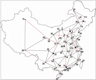
out-Figure 1 shows the optimal solution, where the 6 dis-tribution centers are city 1, city 7, city 10, city 19, city 22 and city 44, and the edges marked by red color represent the delivery routes from each distribution center to its customers.
comes of losing just one edge. One can easily enumerate each of the possible ways of losing one edge as well as calculate the impact of each possible loss in terms of changes in efficiency. The results of this series of calcu-lations will define a range of losses from the best case (i.e. the least decrease in efficiency) to the worst case (i.e. the greatest decrease in efficiency). We then have a re-gion defined by an upper curve and a lower curve, where the upper and the lower curve represent the solutions of the least or the greatest impact associated with a given loss level, respectively. The region depicted between these two curves can be defined as the operational enve-lope or reliability enveenve-lope. For a given edge loss level, this envelope specifies the range of possible system per-formance from the best-case to the worst-case. Actual performance will fall within this range.
Given this operating system of 6 facilities and a poten-tial failure edges set
1 5, 47 , 2 1, 3 , 3 7, 40 , 4 10, 38 , 5 22, 23 , 6 22, 25 , 7 27, 44 ,8 19, 21 ,
F
which is consisted of 8 edges (the sub-graph GF is connected, i.e., both of Nis and NiFs are not ), we
then consider edge loss level from 1 to 8 and solve the worst case DRM and the best case DRM. The solutions are given in Table 1.
In Table 1, for each edge loss level, the objective function values and efficiency for each case are also given as a percentage, where 100% represents the oper-ating level before edge failures. Of cause, the edges shown in volume 6 of Table 1 are the most important objective of protection.
In this section we apply the DRM and the SRM to a data set to generate reliability envelopes. Our data set is derived from the 2008 China census data: a 49-node set consisting of the capitals of all the provinces in China plus the two special administrative regions Hong Kong and Macau, as well as other 15 big cities. The demand of city , i is settled to be the city’s administrative re-gion population divided by 104. The transportation links are the recent national highways and the transportation cost between city and city , equal to the dis-tance between the two cities.
i h
i j dij
Figure 2 presents the values of operational efficien-cies (in percent) as a graph, depicting the lower and the upper boundaries of the reliability envelope. Notice that the greatest marginal impact for the worst case occurs when the edge loss level is small while for the best case occurs when the edge loss level is great.
We optimally solve a 6-median problem in order to
[image:4.595.140.454.444.707.2]obtain an existing facility system. It is also important to note that the greatest difference
Table 1. Results of the worst-case DRM and the best-case DRM.
Level Best-Case Worst-Case
r Objec. Value Failed Edges Efficiency Objec. Value Failed Edges Efficiency
0 11,572,831 - 100% 11,572,831 - 100%
1 11,599,381 6 99.77% 12,989,073 5 89.10%
2 11,669,755 3, 6 99.17% 13,558,323 5, 7 83.54%
3 11,742,050 3, 4, 6 98.56% 13,852,403 2, 5, 7 83.54%
4 11,887,640 3, 4, 6, 8 97.35% 14,059,421 1, 2, 5, 7 82.31%
5 12,051,692 1, 3, 4, 6, 8 96.03% 14,205,011 1, 2, 5, 7, 8 81.47%
[image:5.595.290.536.98.436.2]6 12,345,772 1, 2, 3, 4, 6, 8 93.74% 14,277,306 1, 2, 4, 5, 7, 8 81.06% 7 12,735,040 1, 2, 3, 4, 6, 7, 8 90.87% 14,347,680 1, 2, 3, 4, 5, 7, 8 80.66% 8 14,376,780 1, 2, 3, 4, 5, 6, 7, 8 80.50% 14,376,780 1, 2, 3, 4, 5, 6, 7, 8 80.50%
Figure 2. Reliability envelope of solutions in Table 1.
between the worst case and the best case, or the thickness of the envelop occurs when the edge loss level is moder-ate.
[image:5.595.57.297.102.431.2]By using the same data set as in the above DRM, we then solve the worst case and the best case SRM with edge failure probability p = 0.3 and p = 0.7, respectively. The solutions of the latter and the corresponding reliabil-
Figure 3. Reliability envelope of solutions in Table 2.
ity envelope are showed in Table 2 and Figure 3, re-spectively. Notice that the characteristics of this reliabil-ity envelope are similar to that of the DRM except that, on the same edge loss level, the efficiency losses of the SRM are less than that of the DRM, since we assume that the failure probability of an edge under a strike is 1 in the DRM. We can also observe from Table 2 that, for
Table 2. Results of the worst case SRM and the best case SRM with edge failure probability 0.7.
Level Best-Case Worst-Case
r Objec. Value Attacked Edges Efficiency Objec. Value Attacked Edges Efficiency
0 11,572,831 - 100% 11,572,831 - 100%
1 11,591,416 6 99.84% 12,564,200 5 92.11%
2 11,640,678 3, 6 99.42% 12,915,856 5, 7 89.60%
3 11,691,284 3, 4, 6 98.99% 13,121,712 2, 5, 7 88.20%
4 11,793,197 3, 4, 6, 8 98.13% 13,257,602 1, 2, 5, 7 87.29%
5 11,908,034 1, 3, 4, 6, 8 97.19% 13,359,515 1, 2, 5, 7, 8 86.63%
6 12,113,890 1, 2, 3, 4, 6, 8 95.53% 13,410,122 1, 2, 4, 5, 7, 8 86.30%
7 12,377,354 1, 2, 3, 4, 6, 7, 8 93.50% 13,459,383 1, 2, 3, 4, 5, 7, 8 85.98%
8 13,479,218 1, 2, 3, 4, 5, 6, 7, 8 85.86% 13,479,218 1, 2, 3, 4, 5, 6, 7, 8 85.86%
[image:5.595.102.496.573.717.2]a given edge attacked level, the most important edges of protection are shown in volume 6.
4. Summary and Conclusions
In this paper, we propose two types of scenario based facility location models in order to analyze the reliability of an existing facility system when subject to edge fail-ures. We distinguish deterministic and stochastic cases to formulate and compute a specific example. Reliability envelopes in these two different cases are also given. The information in the reliability envelopes can be very use-ful in looking at ways to protect a facility system. Whether the protection is against a natural disaster or intentional strike, reducing the probability of success even by modest amounts could have an impact on system efficiency. For example, this could be done by placing extra strength in key sections such as bridges or tunnels which spaced in disaster-prone areas, or by adding a surveillance system with guards to help protect against an intruder. Either techniques may not completely elimi-nate a loss, by reduce the edge failure probability to zero, but such strategies may generate more benefits in terms of improved expected system operating efficiencies than what it might cost. Therefore, the value of our analysis could lead to higher levels of safety as well as efficient levels of resource allocation for security measures (whether that involves a possible natural disaster or an attacker).
While a large body of literature focus on the reliable and robust facility system design and analysis under component failures, the existing works are mainly con-centrated on the “node” (e.g., suppliers, distribution cen-ters) losses. To the best of our knowledge, researchers and practitioners have not paid enough attention to the impact of edge failures to facility systems’ efficiency by so far. Comparing to the related works done in this field, our work have at least the following innovations.
Firstly, combining edge failures into facility systems reliability analysis is more realistic than only considering vertex failures. In fact, natural disasters or intentional attacks damage the edges of a facility system more easily. Secondly, in the PMP and other uncapacitated facility location problems, when one or more “nodes” have failed, the overall supplement of the facility system will decrease dramatically but the total demand does not change. If in this situation all demands must to be met, then every node must has no any capacity limit. However, the capacity of nodes are designed a priori, when a vertex failure happen, how can it’s adjacent nodes guarantee the increased demands, let alone more than one vertex fail-ure occur simultaneously?
The recovery time for a failed edge maybe shorter than
that for a failed vertex, but this is not always the case. So we do not explicitly point out the time horizon in our models. In addition, the evaluation of edge failure prob-ability is important and difficult, and we will discuss this question in another work. We set the failure probability of all edges as the same when solving the example since we aimed to demonstrate the impact of edge failures to the efficiency of a facility system.
5. Acknowledgements
This paper was supported by the Open Fund of Xi’an Jiaotong University (No. 2010-4), SXESF (No. 09JK545) and BSF (No. JC0924).
6. References
[1] R. L. Church and M. P. Scaparra, “Critical Infrastruc-ture,” Springer, Berlin, 2007.
[2] R. Kembel, “The Fibre Channel Consultant: A Compre-hensive Introduction,” Northwest Learning Associates, Tucson, 2000.
[3] Y. Sheffi, “The Resilient Enterprise: Overcoming Vul-nerability for Competitive Advantage,” MIT Press, Cam-bridge, 2005.
[4] M. Bundschuh, D. Klabjan and D. L. Thurston, “Model-ing Robust and Reliable Supply Chains,” Work“Model-ing Paper, University of Illinois, Urbana-Champaign, 2003.
[5] L. V. Snyder and Z. J. M. Shen, “Managing Disruptions to Supply Chains,” The Bridge (National Academy of En-gineering), Vol. 36, No. 4, 2006, pp. 39-45.
[6] S. L. Hakimi, “Optimum Location of Switching Centers and the Absolute Centers and Medians of a Graph,” Op-erations Research, Vol. 12, No. 3, 1964, pp. 450-459.
[7] S. L. Hakimi, “Optimum Distribution of Switching Cen-ters and Some Graph Related Theoretic Properties,” Op-erations Research, Vol. 13, 1965, pp. 462-475.
[8] M. B. Teitz and P. Bart, “Heuristic Methods for Estimat-ing the Generalized Vertex Median of a Weighted Graph,”
Operations Research, Vol. 16, No. 5, 1968, pp. 955-961.
doi:10.1287/opre.16.5.955
[9] C. S. Revelle and R. Swain, “Central Facilities Location,”
Geographical Analysis, Vol. 2, No. 1, 1970, pp. 30-42.
doi:10.1111/j.1538-4632.1970.tb00142.x
[10] R. L. Church, “COBRA: A New Formulation for the Classic p-Median Location Problem,” Annals of Opera-tions Research, Vol. 122, No. 1-4, 2003, pp. 103-120.
doi:10.1023/A:1026142406234
[11] R. D. Carr, et al., “Robust Optimization of Contaminant Sensor Placement for Community Water Systems,” Mathe- matical Programming, Vol. 107, No. 1-2, 2005, pp. 337- 356.
Optimization, Vol. 6, No. 1, 2002, pp. 81-98.
doi:10.1023/A:1013322309009
[13] R. L. Church, M. P. Scaparra and R. S. Middleton, “Iden-tifying Critical Infrastructure, The Median and Covering