A Comparative Study of Nonlinear Time-Varying Process
Modeling Techniques: Application to Chemical Reactor
Errachdi Ayachi, Saad Ihsen, Benrejeb Mohamed
LARA Automatique, Tunis, Tunisia.
Email: [email protected], [email protected], [email protected]
Received December 27th, 2010; revised May 12th, 2011; accepted May 22nd, 2011
ABSTRACT
This paper proposes the design and a comparative study of two nonlinear systems modeling techniques. These two ap- proaches are developed to address a class of nonlinear systems with time-varying parameter. The first is a Radial Basis Function (RBF) neural networks and the second is a Multi Layer Perceptron (MLP). The MLP model consists of an input layer, an output layer and usually one or more hidden layers. However, training MLP network based on back propagation learning is computationally expensive. In this paper, an RBF network is called. The parameters of the RBF model are optimized by two methods: the Gradient Descent (GD) method and Genetic Algorithms (GA). However, the MLP model is optimized by the Gradient Descent method. The performance of both models are evaluated first by using a numerical simulation and second by handling a chemical process known as the Continuous Stirred Tank Reactor CSTR. It has been shown that in both validation operations the results were successful. The optimized RBF model by Genetic Algorithms gave the best results.
Keywords: Nonlinear Systems; Time-Varying Systems; Multi Layer Perceptron; Radial Basis Function; Gradient
Descent; Genetic Algorithms; Optimization
1. Introduction
Neural networks are widely used in the characterization of nonlinear systems [1-7], time-varying time-delay non- linear systems [8] and they are applied in various appli- cations [9-12].
The system may be with invariant parameters or time- varying parameters. The variation of some system may be such as; system with slow time-varying parametric uncertainties [13,14], with arbitrarily rapid time-varying parameters in a known compact set [15], with rapid time- varying parameters which converge asymptotically to constants [16], and with unknown parameters with arbi- trarily fast and nonvanishing variations [17].
Using MLP architecture depends on various parame- ters, for instance the number of hidden layers, the num- ber of neurons in each hidden layers, the activation func- tion and the learning rate. These parameters present a difficulty to find the suitable architecture of the MLP.
A renewed interest in Radial Basis Function (RBF) neural network has been found in recent years in various application areas such as modeling and control [1-2], pattern recognition [18] identifying malfunctions of dy- namical systems in the case of the frequency multiplier [19], and in the case of jump phenomenon [20], deter- mining the optimal choice of machine tools [21], pre-
dicting 2D structure of proteins [22], classification [23, 24], solving systems of equations [25], analysis of the interaction of multi-input multi-output [26] and modeling of robots [27].
Using an RBF leads to a general model structure is less complex than that produced by an MLP network. The computational complexity induced by their learning is less than that induced by learning the MLP networks. The RBF network performance depends, to a choice of activation function [1], the number of hidden neurons and synaptic weights. By the time-varying nature of pa- rameters the RBF methods are not applicable. However, the RBF is well used in invariant-system. The MLP is used in estimation of time-varying time-delay nonlinear system [17]. In this work, we investigate the possibility of extending the well conventional methods to model a nonlinear system in presence of time-varying parameters.
Several methods such as iterative methods [28-32] with the gradient descent method and evolutionary algo- rithms [32] that genetic algorithms are used in this paper to optimize the structure and determine the parameters of the RBF model. On the other hand, the gradient descent method is used to optimize the MLP network [33].
chitecture. The proposed algorithms are applied to time- varying nonlinear systems. The RBF using genetic algo- rithms gave the best results.
This paper is organized as follows. Nonlinear system modeling by MLP and RBF network is presented at the second and the third section. A comparative study be- tween the MLP and RBF model, applied to two examples of nonlinear systems is presented in the forth section. Conclusions are given in the fifth section.
2. Nonlinear System Modeling by MLP
Modeling a nonlinear system from its input-output can be for several models. Among these models, the NARMA (Nonlinear Auto-Regressive Moving Average) [19] is used; its expression is given by the following equation:
1
, , y 1 , , , u 1
y k
f y k y k N u k u k N
(1)
where f is a nonlinear mapping, u k
and y k
are the input and output vector, Nu and Ny are the maximum input and output lags, respectively. In this paper, the coefficients of the model (1) depend on time.
The used MLP in this paper is to describe the nonlin- ear system (1). The objective of the modeling is to obtain an MLP that its output follows the output of the system.
2.1. Structure of MLP
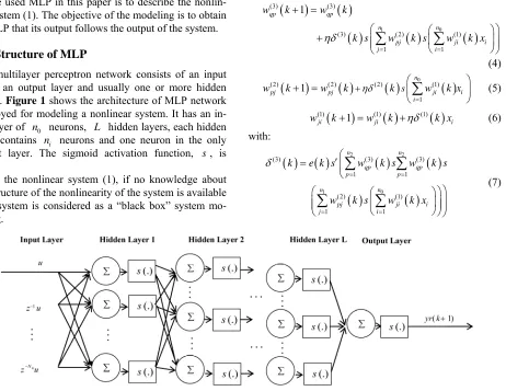
The multilayer perceptron network consists of an input layer, an output layer and usually one or more hidden layers. Figure 1 shows the architecture of MLP network
employed for modeling a nonlinear system. It has an in- put layer of 0 neurons, hidden layers, each hidden
layer contains i neurons and one neuron in the only output layer. The sigmoid activation function,
n n
L
s, is
used.
For the nonlinear system (1), if no knowledge about the structure of the nonlinearity of the system is available such system is considered as a “black box” system mo- deling.
The output of MLP model is given by the
following equation:
1
yr k
0
2 1
( 1) (3) (2) (1)
1
1 1 1 1
1
L n
n n n
L
l qp pj ji i
l p j i
yr k
s w s w s w s w x
(2)
where s is a sigmoid activation function, yr k
(2) is the output vector of MLP. 1
L , p , (L 1)
w (3)
q w
pj and
w (1)
ji
are the synaptic weights of MLP.
w
i
x is the input vector
of MLP.
2.2. Optimization of MLP
Among the optimization methods of MLP, the gradient descent method is used in this paper. Optimization of the MLP is to minimize the mean square error E.
2
20 0
1 1
2 2
N N
k k
E k e k y k yr k
(3)
where E is a function cost.
In this section, 2 hidden layers are taken into account with a single input layer and one output layer, the result of optimization is given by Equations (4) to (10):
1
0
(3) (3)
(3) (2) (1)
1 1
1
qp qp
n n
pj ji i
j i
w k w k
k s w k s w k x
(4)
0
(2) (2) (2) (1)
1
1
n
pj pj ji
i s
w k w k k w k x
i (5)
(1) 1 (1) (1)
ji ji
w k w k k xi (6)
with:
2 2
0 1
(3) (3) (3)
1 1
(2) (1)
1 1
n n
qp qp
p p
n n
pj ji i
j i
k e k s w k s w k
w k s w k x
s
(7) [image:2.595.81.543.368.725.2]
1
0
(2) (2) (1)
1 1
n n
pj ji i
p i
k e k s w k s w k x
(8)
0
(1) (1)
1
n
ji i
i
k e k s w k x
(9)
. . 1
.
s s s (10)
3. Nonlinear System Modeling by RBF
As we did with the MLP model, the RBF is used to de- scribe the nonlinear system (1).
3.1. Structure of RBF
The RBF consists of only three layers; an input layer, an output layer and usually one hidden layers contains a hidden radial basis function. The RBF model calculates a linear combination of radial basis functions as is given by the following equation:
11
1 j j
n
j
ym k v
(11)where ym k
is the output vector of RBF. vj is thesynaptic weights of RBF and j is a Gaussian activa- tion function:
22 exp 2 j j j x
(12)
3.2. Optimization Methods of RBF
Compared to the MLP, the RBF contains a very small number of parameters. The purpose of optimizing RBF is to determine j, j and vj by minimizing the func- tion cost E.
12 1 1 2 1 1 1 1 2 2 1 2 N N k k n N j j k j
E e k y k ym k
y k v
2 (13)In order to find the minimum of j, j and vj
two strategies are proposed in the literature for finding the minimum of . The first is based on supervised methods or algorithms using direct time-consuming cal- culation to determine the minimum of . The second adopts a hybrid scheme (less costly in computation time) to determine the minimum of . Solving these prob- lems can be by various methods such as iterative meth- ods (the Gradient Descent method) and evolutionary al- gorithms (Genetic Algorithm).
E
E
E
3.2.1. Optimization of RBF Using Gradient Descent
The principle of the GD method is applied to optimize the parameters of the RBF model. It uses the rules of delta:
1j j E v k v
(14)
2j j E k
(15)
3j j E k
(16)
Hence the calculation of partial derivatives introduced by the following equations:
11 n j j j j E
y k v
v j
(17)
12
3
1
n j
j j j j
j
j j
x E
v y k v
(18)
12
1
n j
j j j j
j
j j
x E
v y k v
(19)finally, we obtain
1
1j j
j
E
v k v k
v
(20)
1
2j j j E k k
(21)
1
3j j j E k k
(22)
The learning rate i satisfies the following condition: 0i1 i1, 2,3 (23)
E is nonlinear in the parameters, which calls for
finding the minimum, the use of an iterative algorithm that requires an arbitrary initialization of RBF network parameters and a suitable choice of i. To maximize the chances of finding the global minimum of , several initialization parameters and therefore more training is needed, which increases the computing time.
E
Another method is to optimize separately the parame- ters of the hidden layer (the centers and the widths ) by genetic algorithms and the synaptic weights be- tween the hidden layer and output layer by the gradient descent method.
3.2.2. Optimization of RBF Using Genetic Algorithms
tion: crossover, mutation, selection. The GA is often used for optimization of RBF [34-38].
In this paper, the GA is used in order to optimize sep-arately the parameters of the hidden layer (the centers and the widths ) of the RBF model.
To find suitable parameters, five elements of GA are called:
A population is generated randomly. The population size is chosen to achieve a compromise between com- putation time and solution quality.
The evaluation of each individual is performed by an evaluation function called fitness function. This func- tion represents the only link between the physical problem and GA. In this paper, the used fitness func- tion is given by the following equation.
2 21 2 sin 0.9 1
gx x x (24)
with x1 and x2 are respectively the and the
which are used also in the following equation:
1
2 2
2
1 1
1 exp
2 2
n
N j
j
k j j
x
E y k v
(25)
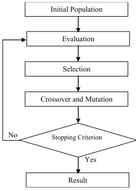
Once the evaluation of generation is realized, it makes a selection from the fitness function. In this paper, the tournament selection is used.
The crossover operator is designed to enrich the di- versity of the population by manipulating the genes of individuals existing in the population. In the other hand, the mutation operator involves the inversion of a bit in a chromosome. The mutation that mathemati- cally guarantees the global optimum can be reached. The stopping criterion indicates that the solution is
[image:4.595.352.490.85.279.2] [image:4.595.308.535.382.508.2]sufficiently approximate the optimum. In this paper, the maximum number of generations is chosen as stopping criterion.
Figure 2 shows the organization of GA to find the
mi-nimal parameters of the hidden layer.
The obtained parameters (, ) by GA are used also in the following equation:
1
2
2 1
1 exp
2 n
j
j j
x ym k
(26)and the synaptic weights are calculated using the gradient descend method:
11
1
1 n
j j j
j
v k v k y k vj j
(27)4. Comparative Study of Models
The effectiveness of the suggested methods applied to
No
Yes Initial Population
Evaluation
Selection
Crossover and Mutation
Stopping Criterion
Result
Figure 2. Organization of genetic algorithm.
the identification of behavior of two nonlinear time- va-rying systems are demonstrated by simulation experi- ments.
The performance of MLP and RBF models are evalu- ated by Normalized root Mean Square Error between the system output and the model output, denoted NMSE.
2
1
2
1
N
k
MLP N
k
y k yr k NMSE
y k
(28)and
2
1
2
1
N
k
RBF N
k
y k ym k NMSE
y k
(29)4.1. Nonlinear Time Varying-System
We consider the nonlinear time-varying system described by input-output model:
2
2
0 1
1
1 2 1 2 1
1 1 2
y k
y k y k y k u k y k u k
a k y k a k y k
(30) with:
0
1
1 0.2 cos 1 0.2sin
a k k
a k k
(31)
The trajectory of a0
k and a k1
are given inFigure 3.
The input u k
is sinusoidal signal and it is defined0 50 100 150 200 250 300 -0.2
-0.1 0 0.1 0.2
k
a0
(k
)
0 50 100 150 200 250 300
0 0.5 1 1.5
k
a1
(k
[image:5.595.170.428.87.274.2])
Figure 3. a0(k) and a1(k) trajectories.
0.325sin 0.95 cos 0.55
u k k k
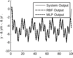
(32)In Figure 4, the time-varying system responses, the
MLP model and the optimized RBF model by the GD method are presented. In this simulation figure, the MLP parameters are n06, n115, n220 and
0.44
. The obtained EMLP
1 0.3
NMS is .
However, the RBF parameters are
3
2.78 10 %
4
, 2 0.01
and 3 0.002. The obtained NMSERBF is .
3%
3.9812 10
In Figure 5, the time-varying system responses, the
MLP model and the optimized RBF model by GA are illustrated. In this simulation the same MLP parameters are taken, while the RBF parameters are 1 0.172,
, and
0.7
Pc Pm0.1 T 100. The obtained
RBF
In these two Figures (4 and 5), it is clear that the
sponses of MLP and RBF models follow the system re-sponse although the variation of parameters.
NMSE is 2.0210 %3 .
In one hand, the obtained MLP model is found by sev-eral tests of parameters and of learning. The large num-ber of MLP parameter increases the difficulty of its use. However, the simplicity of RBF makes modeling is sim-ple and takes much less training time.
In Figure 4, the optimized RBF model by the gradient
descent method depends on an expensive time of training and depends on different learning rate ( 1 0.34,
2 0.01
and 3 0.002) while, in Figure 5, the
pa-rameter of RBF model ( and ) are finding sepa-rately by the GA and the synaptic weights ( ) by the DG method, hence the model is faster than the previous.
v
Noise Effect of Time-Varying Nonlinear System
To validate the quality of the proposed algorithm, an added white noise is used. The influence of the noise of modeling, the Signal Noise Ratio (SNR) is used. The
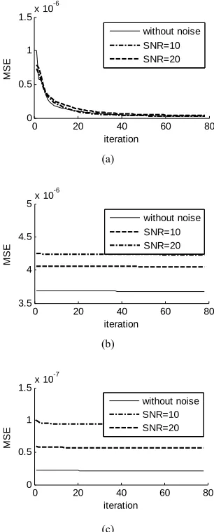
Figures 6(a)-(c) present the evolution of
dif-ferent SNR for the both models.
NMSE
2
1
2
1
SNR N
k N
k
y k y
k
(33)where y and are respectively the output average
value and noise average value.
0 20 40 60 80 100
-8 -6 -4 -2 0 2
k
y
- &
y
m
-.
&
y
r .
[image:5.595.347.497.425.540.2]System Output RBF Output MLP Output
Figure 4. The responses of time-varying system, MLP mo- del and the optimised RBF model by GD.
0 20 40 60 80 100
-10 -8 -6 -4 -2 0 2
k
y
&
ym
-. &
yr
.
System Output RBF Output MLP Output
[image:5.595.348.496.587.704.2]0 20 40 60 80 0
0.5 1 1.5x 10
-6
iteration
MS
E
without noise SNR=10 SNR=20
(a)
0 20 40 60 80
3.5 4 4.5
5x 10
-6
iteration
MS
E
without noise SNR=10 SNR=20
(b)
0 20 40 60 80
0 0.5 1 1.5x 10
-7
iteration
MS
E
without noise SNR=10 SNR=20
(c)
Figure 6. Evolution of MSE of different SNR: (a) MLP; (b) Optimized RBF model with GD method; (c) Optimized RBF model with GA.
In these three Figures 6(a)-(c), we remark firstly the
error goes down when the SNR value goes high, then the lowest MSE is obtained when the GA is used (Figure 6(c)). Finally, in these all figures we see that the re-
sponses of MLP and RBF models follow the time-vary- ing system response despite of the variation of parame- ters and an added noise.
4.2. Chemical Reactor
To test the effectiveness of the MLP and RBF models we test them on a Continuous Stirred Tank Reactor, CSTR, which is a type of slowly time-varying nonlinear system used for the conduct of the chemical reactions [39-41]. However, the input-output are used in discrete time. A diagram of the reactor is given in the Figure 6. The
physical equations describing the process are (34) and (35):
1 2
d
0.2 d
h t
w t w t h t
t (34)
1 2
1 2
1
2 2
d d
1 b
b b b b
b
b
C t w t w t
C C C C
t h t
k C t
k C t
h t
(35)
where h t
is the height of the mixture in the reactor,
1
w t (respectively w t2
C
) is the feed of reactant 1 (respectively reactant 2) and b1 (respectively b2) is
the concentration of reactant 1(respectively reactant 2). is the feed product of reaction and its concentration is
b. 1, 2, 2 and b2 are consumption reactant
rate. They are assumed to be constant. The temperature in the reactor is assumed constant and equal to the ambi- ent temperature. The feed of reactant 1 and the con-
centration b1 are the input of the process however b represents its output. A diagram of the reactor is given in the Figure 7.
C C
w
C k k
C w
w
C
For the purpose of the simulations the CSTR model of the reactor provided with Simulink-Matlab is used.
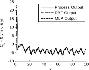
In Figure 8, the responses of the chemical reactor, the
model that produced by MLP and optimized RBF model by the gradient descent method are presented. In Figure 9, the responses of the chemical reactor, the MLP model
and the optimized RBF model by genetic algorithms are illustrated.
In Figures 8 and 9, the responses of the optimized
RBF model by the GD method and MLP model follow the response of chemical reactor. Indeed, in Figure 8, the
MLP model is carried out with 5 neurons in input layer, 25 neurons in first hidden layer, 22 neurons in hidden layer and the learning rate equal to 0.4. However, the RBF model depends only 3 layers, the second and the only hidden layer contains 11 neurons. The used para- meters in the GD method are 1 0.37, 2 0.003
and 3 0.02. In contrary, in Figure 9, the parameter of
w1: Feed of reactant 1
Cb1:Concentration of reactant 1
w2: Feed of reactant 2
Cb2: Concentration of reactant 2
w: Feed Product Cb: Product Concentration
[image:6.595.333.539.87.182.2]h
[image:6.595.95.248.88.468.2] [image:6.595.307.539.561.715.2]0 20 40 60 80 100 -10
-5 0 5 10 15 20 25
k
Cb
& y
m
-. & y
r .
[image:7.595.93.250.89.213.2]Process Output RBF Output MLP Output
Figure 8. The responses of process, MLP model and the op- timized RBF model by GD.
0 20 40 60 80 100
-10 -5 0 5 10 15 20 25
k
Cb
& y
m
-. &
y
r
.
[image:7.595.91.254.259.387.2]Process Output RBF Output MLP Output
Figure 9. The responses of process, MLP model and the op- timized RBF model by GA.
RBF model are optimized separately ( and ) using GA and (v) using gradient descent. These parameters are
1 0.11
, Pc0.8, Pm0.2 and T 100. The NMSE is given in the table below:
- MLP RBF + GD RBF + GA
NMSE (%) 1.45e−003 5.97e−002 2.50e−002
From this table, the NMSE computed in the RBF
mod-el optimized by the genetic algorithms method is lower than that found by applying the gradient descent method which proves that the evolutionary algorithms give good accuracy for modeling methods of dynamical systems.
5. Conclusion
This paper has dealt with the study and the comparison of two systems modeling techniques the multilayer net-work model and the radial basis function neural netnet-work model. These two approaches are applied in a class of nonlinear system with time-varying parameters. It has been shown that the MLP architecture depends on vari- ous parameters and of course a much training time. However, the RBF model depends on the synaptic weights, center and width of its function. In this paper, the RBF
model is optimized by gradient descent method and ge- netic algorithms. Each optimized RBF models are com- pared with multilayer perceptron. Mean square error is carried out to evaluate performance of both models and the influence of an additive noise on the identification qualities. These models have been tested for modeling of chemical reactor and results are successful. The RBF model optimized by genetic algorithms showed good performance compared to that optimized by gradient de- scent method.
REFERENCES
[1] V. T. S. Elanayar and C. S. Yung, “Radial Basis Function Neural Network for Approximation and Estimation of Nonlinear Stochastic Dynamic,” IEEE Transactions on Neural Networks, Vol. 5, No. 4, 1994, pp. 594-603. doi:10.1109/72.298229
[2] P. Borne, M. Benrejeb and J. Haggege, “Les Réseaux de Neurones. Présentation et Applications,” Editions Ophrys, Paris, 2007.
[3] S. Chabaa, A. Zeroual and J. Antari, “Identification and Prediction of Internet Traffic Using Artificial Neural Networks,” Journal of Intelligent Learning Systems & Applications, Vol. 2, No. 3, 2010, pp. 147-155.
[4] A. Errachdi, I. Saad and M. Benrejeb, “On-Line Identifi- cation Method Based on Dynamic Neural Network,” In- ternational Review of Automatic Control, Vol. 3, No. 5,
2010, pp. 474-479.
[5] H. Vijay and D. K. Chaturvedi, “Parameters Estimation of an Electric Fan Using ANN,” Journal of Intelligent Learning Systems & Applications, Vol. 2, No. 1, 2010, pp.
43-48.
[6] A. Mishra and Zaheeruddin, “Design of Hybrid Fuzzy Neural Network for Function Approximation,” Journal of Intelligent Learning Systems & Applications, Vol. 2, No.
2, 2010, pp. 97-109.
[7] A. Errachdi, I. Saad and M. Benrejeb, “Internal Model Control for Nonlinear Time-Varying System Using Neu- ral Networks,” 11th International Conference on Sciences and Techniques of Automatic Control & Computer Engi- neering, Monastir, 19-21 December 2010, pp. 1-13.
[8] Y. Tan, “Time-Varying Time-Delay Estimation for Non- linear Systems Using Neural Networks,” International Journal of Applied Mathematics and Computer Science,
Vol. 14, No. 1, 2004, pp. 63-68.
[9] R. Sollacher and H. Gao, “Towards Real-World Applica- tions of Online Learning Spiral Recurrent Neural Net- works,” Journal of Intelligent Learning Systems & Ap- plications, Vol. 1, No. 1, 2009, pp. 1-27.
[10] S. H. Ling, “A New Neural Network Structure: Node-to- Node-Link Neural Network,” Journal of Intelligent Learn- ing Systems & Applications, Vol. 2, No. 1, 2010, pp. 1-
11.
Sys-tems & Applications, Vol. 2, No. 1, 2010, pp. 12-18.
[12] K. N. Sujatha and K. Vaisakh, “Implementation of Adap- tive Neuro Fuzzy Inference System in Speed Control of Induction Motor Drives,” Journal of Intelligent Learning Systems & Applications, Vol. 2, No. 2, 2010, pp. 110-
118.
[13] R. H. Middleton and G. C. Goodwin, “Adaptive Control of Time-Varying Linear Systems,” IEEE Transactions on Automatic Control, Vol. 33, No. 2, 1988, pp. 150-155.
doi:10.1109/9.382
[14] F. Giri, M. Saad, J. M. Dion and L. Dugard, “Pole Place- ment Direct Adaptive Control for Time-Varying Ill-Mod- eled Plants,” IEEE Transactions on Automatic Control,
Vol. 35, 1990, pp. 723-726. doi:10.1109/9.53553
[15] K. S. Tsakalis and P. A. Ioannou, “Linear Time-Varying Systems: Control and Adaptation,” Prentice-Hall, Upper Saddle River, 1993.
[16] R. Marino and P. Tomei, “Adaptive Control of Linear Time-Varying Systems,” Automatica, Vol. 39, No. 4, 2003,
pp. 651-659. doi:10.1016/S0005-1098(02)00287-X [17] R.-H. Chi, S.-L. Sui and Z.-S. Hou, “A New Discrete-
Time Adaptive ILC for Nonlinear Systems with Time- Varying Parametric Uncertainties,” ACTA Automatica Si- nica, Vol. 34, No. 7, 2008, pp. 805-808.
doi:10.3724/SP.J.1004.2008.00805
[18] M. R. Berthold, “A Time Delay Radial Basis Function Network for Phoneme Recognition,” IEEE Rerthold Intel Corporation, Santa Clara, 1994, pp. 4470-4472.
[19] M. Zarouan, J. Haggège and M. Benrejeb, “Anomalies de Fonctionnement de Systèmes Dynamiques et Modélisa- tion par Réseaux de Neurones des Non-Linearités: Cas de la Démultiplication de Fréquence,” Premières Journées Scientifiques des Jeunes Chercheurs en Genie Electrique et Informatique, 23-24 March 2001, Sousse-Tunisie, pp.
123-128.
[20] J. Haggège, M. Zarouan and M. Benrejeb, “Anomalies de Fonctionnement et Modélisation de systèMes Dynamiques par réSeaux de Neurones: Cas du Phénomène de Saut,”
Premières Journées Scientifiques des Jeunes Chercheurs en Genie Electrique et Informatique, 23-24 March 2001,
Sousse-Tunisie, pp. 134-138.
[21] S. Allali and M. Benrejeb, “Application des Réseaux de Neurones Multicouches pour le Choix Optimal des Ma- chines Outils,” 4 ème Conférence Internationale JTEA,
Hammamet, 12-14 March 2006.
[22] H. Bouziane, B. Messabih and A. Chouarfia, “Prédiction de la Structure 2D des Protéines par les Réseaux de Neu- rones,” Communications of the IBIMA, Vol. 6, 2008, pp.
201-207.
[23] J. Park and I. Sandberg, “Universal Approximation Using Radial-Basis-Function Networks,” Neural Computation,
Vol. 3, No. 2, 1991, pp. 246-257. doi:10.1162/neco.1991.3.2.246
[24] A. Sifaoui, A. Abdelkrim, S. Alouane and M. Benrejeb, “On new RBF Neural Network Construction Algorithm for Classification,” SIC, Vol. 18, No. 2, 2009, pp. 103-
110.
[25] A. Golbabai, M. Mammadov and S. Seifollahi, “Solving a
System of Nonlinear Integral Equations by an RBF Net-work,” Computer and Mathematics with Applications,
Vol. 57, No. 10, 2009, pp. 1651-165. doi:10.1016/j.camwa.2009.03.038
[26] X. Chengying and C. S. Yung, “Interaction Analysis for MIMO Nonlinear Systems Based on a Fuzzy Basis Func- tion Network Model,” Fuzzy Sets and Systems, Vol. 158,
No. 18, 2007, pp. 2013-2025. doi:10.1016/j.fss.2007.02.012
[27] S. S. Chiddarwar and N. R. Babu, “Comparison of RBF and MLP Neural Networks to Solve Inverse Kinematic Problem for 6R Serial Robot by a Fusion Approach,” En- gineering Applications of Artificial Intelligence, Vol. 23,
No. 7, 2010, pp. 1-10.
[28] R. P. Brent, “Fast Training Algorithms for Multilayer Neural Net,” IEEE Transactions on Neural Networks, Vol.
5, No. 6, 1991, pp. 989-993.
[29] M. T. Hagan and M. Menhaj, “Training Feedforward Networks with Marquardt Algorithm,” IEEE Transac- tions on Neural Networks, Vol. 5, No. 6, 1994, pp. 989- 993. doi:10.1109/72.329697
[30] R. A. Jacobs, “Increased Rates of Converge through Learn- ing Rate Adaptation,” Neural Networks, Vol. 1, No. 4,
1988, pp. 295-307. doi:10.1016/0893-6080(88)90003-2 [31] D. C. Park., M. A. El Sharkawi and R. J. Marks II, “An
Adaptively Trained Neural Network,” IEEE Transactions on Neural Networks, Vol. 2, No. 3, 1991, pp. 334-345.
doi:10.1109/72.97910
[32] M. Schoenauer and Z. Michalewicz, “Evolutionary Com- putation,” Control and Cybernetics, Vol. 26, No. 3, 1997,
pp. 307-338.
[33] A. Errachdi, I. Saad and M. Benrejeb, “Neural Modeling of Multivariable Nonlinear System. Variable Learning Rate Case,” Intelligent Control and Automation, Vol. 2, No. 3, 2011, pp. 165-175.
[34] W. L. Cheol and C. S. Yung, “Growing Radial Basis Func- tion Networks Using Genetic Algorithm and Orthogo- nalization,” International Journal of Innovative Com- puting, Information and Control ICIC International, Vol.
5, No. 11A, 2009, pp. 3933-3948.
[35] G. Lin, H. De-Shuang and Z. Wenbo, “Combining Ge- netic Optimization with Hybrid Learning Algorithm for Radial Basis Function Neural Networks,” Electronic Let- ters, Vol. 39, No. 22, 2003, pp. 1600-1601.
[36] T. Renato and O. M. J. Luiz, “Selection of Radial Basis Functions via Genetic Algorithms in Pattern Recognition Problems,” 10th Brazilian Symposium on Neural Net- works, Salvador, 26-30 October 2008, pp. 71-176.
[37] M. L. Huang and Y. H. Hung, “Combining Radial Basis Function Neural Network and Genetic Algorithm to Im- prove HDD Driver IC Chip Scale Package Assembly Yield,” Expert Systems with Applications, Vol. 34, No. 1,
2008, pp. 588-595. doi:10.1016/j.eswa.2006.09.030 [38] R. Niranjan and G. Ranjan, “Filter Design Using Radial
[39] C. Junghui and H. Tien-Chih, “Applying Neural Net-works to On-Line Updated PID Controllers for Nonlinear Process Control,” Journal of Process Control, Vol. 14,
No. 2, 2004, pp. 211-230.
doi:10.1016/S0959-1524(03)00039-8
[40] J. Van Grop, J. Schoukens and R. Pintelon, “Learning
Neural Networks with Noise Inputs Using the Errors in Variables Approach,” IEEE Transactions on Neural Net- works, Vol. 11, No. 2, 2000, pp. 402-414.
doi:10.1109/72.839010
[41] H. Demuth, M. Beale and M. Hagan, “Neural Network Toolbox 5,” User’s Guide, The MathWorks, Natick, 2007.
Nomenclature
: learning rate,: regularization coefficient,
y k : process output,
u k : process input, ym k
: output of RBF,f : unknown function, j: hidden radial basis function,
: hidden center, y
N : output delay, j
: hidden width, u
N : input delay, NuNy, j
v
yr k : output of MLP,
x
j: synaptic weights of RBF,
Pc: crossover probability,
: input vector of (MLP or RBF),
Pm: mutation probability, L: number of hidden layer,
T: size generation, 0
n n
: number of nodes of input layer, : white noise,
i
n
: number of nodes of hidden layer,
N: number of observations,
: number of nodes of output layer, SNR: Signal Noise Ratio.