Abstract—This paper investigates inventory control policies in a manufacturing/remanufacturing system during the product life-cycle, which consists of four phases: introduction, growth, maturity, and decline stages. Both demand rate and return rate of products are random variables with normal distribution, and the mean of the distribution also varies according to the time in the product life-cycle. Closed-form formulas of optimal production lot size, reorder point, and safety stock in each phase of product life-cycle are derived. A numerical example is presented. The result shows that different inventory control policies should be adopted in different phases of product life-cycle.
Index Terms—inventory, product life-cycle, remanufacturing, reverse logistics
I. INTRODUCTION
For the last decades, many electronic companies encountered two major pressures: shortening product life-cycle and environmental sustainability. Inventory management under short product life-cycle is not easy. It is necessary to consider the constantly varying demand and its uncertainty when making inventory control policy. Due to short product life-cycle, the product may be returned even if it is still in good condition. On the other hand, many companies are required to conform to the Waste of Electric and Electronic Equipment (WEEE) directives in many countries. Environmental sustainability and green supply chain management have become more and more important and have received increasing attention since 1990s [1]. Several international journals have published special issues about sustainable/green supply chain management in recent years [2]-[5]. Two review articles also provide deep discussion about sustainable supply chain management [1], [6]. These articles indicate that the global trend of environmental sustainability is inevitable.
The pressures from shortening product life-cycle and environmental sustainability make remanufacturing become a reasonable choice. Remanufacturing is an industrial process where used/broken products are restored to useful life. Remanufacturing is also an important part of sustainable supply chain and reverse logistics. The motives for product remanufacturing include legislation, increased profitability, ethical responsibility, secured spare part supply, brand
Manuscript received January 28, 2010. This work was supported in part by the National Science Council of Taiwan under Grant NSC 98-2410-H-231-004.
C.-F. Hsueh is with the Department of Marketing and Distribution Management, Ching Yun University, Taoyuan 32097, Taiwan. E-mail: [email protected].
protection, and the reasons for returning used products include end-of-life returns, end-of-use returns, commercial returns, and re-usable components [7]. After remanufacturing, the returned products, together with the new products, compose the serviceable inventory and satisfy the customers’ demand. Inventory control in such remanufacturing systems becomes complicated and receives a lot of attention.
In literature of inventory control with remanufacturing, there are two different assumptions about returned products: one is as-good-as-new and the other is not. Under “as-good-as-new” assumption, the used products are collected and remanufactured to as-good-as-new state. The customers cannot distinguish ‘‘new’’ (‘‘manufactured’’) and ‘‘remanufactured’’ (‘‘repaired’’) products, or they consider these two products as being interchangeable. In this paper, we also apply this assumption to the analysis procedure. The relevant literature in this field is reviewed in the following. Reference [8] considers several inventory control strategies with remanufacturing and disposal. The product demands and product returns are assumed to be independent Poisson processes. Later, the PUSH and PULL strategies are considered in the inventory model to coordinate production, remanufacturing and disposal operations efficiently [9]-[10], although the strategies may still be non-optimal. Lead-time effects are further investigated in a similar remanufacturing system to improve the system performance [11]-[12]. Recently, reference [13] studies a single-echelon inventory system with disposal for remanufacturing. It compares the disposal strategy with the non-disposal strategy and investigates the robustness of the optimal solution. Reference [14] studies joint procurement and production decisions in remanufacturing under quality and demand uncertainty.
All above articles assume that demand rate and return rate are independent. To improve this improper assumption, [15] develops an inventory model in which the random returns depend explicitly on the demand stream. It assumes a constant probability that an item is returned. Reference [16] considers inventory strategies for a reverse logistics system, in which demand is a known continuous function in a given planning horizon and the return rate of used items is also a given function of time; there is a constant delay between these two functions.
As to our knowledge, there is no article that considers product life-cycle in inventory control with remanufacturing. Most articles assume that demand rate and return rate follow specific distributions with fixed parameters, which are consistent through product life-cycle. Although [17] has developed strategies to balance supply and demand for remanufactured products during life-cycle, it does not present a clear inventory control policy.
Inventory Control for Stochastic Reverse
Logistics with Product's Life Cycle
The purpose of this paper is to investigate the effects of product life-cycle on inventory control in a manufacturing/remanufacturing system and to determine the optimal production lot size, reorder point, and safety stock during each phase of product life-cycle. The remainder of the paper is organized as follows. Section 2 presents the assumptions and notations. Section 3 is for mathematical modeling. Section 4 is for numerical examples. Finally, the paper summarizes and concludes in Section 5.
II. ASSUMPTIONS AND NOTATIONS
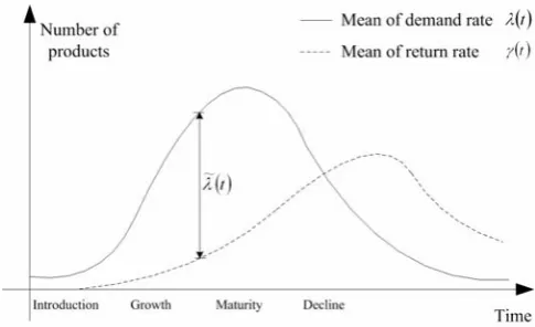
[image:2.595.47.287.427.530.2]The scheme of the manufacturing/remanufacturing system in this paper is illustrated in Fig. 1. The serviceable inventory stocks the manufactured and remanufactured products to satisfy the demand. There are two sources to replenish the serviceable inventory; one is manufacturing new products and the other is remanufacturing the returned products. The remanufactured products are assumed to be as good as new ones. We also assume that both demand rate and return rate of products are random variables with normal distribution, and the mean of the distribution also varies according to the time in the product life-cycle, as illustrated in Fig. 2. We can see that the return rate is not independent to the demand rate. There is a time lag between two functions, and the peak of return rate function is lowered. The product life-cycle is composed of four phases (i.e., introduction, growth, maturity, and decline) and is distinguished by the sales or the demand over time.
Fig. 1 Scheme of the manufacturing/remanufacturing system
Fig. 2 Product life-cycle and the relation between demand rate and return rate
Other assumptions include: (1) the lead time for manufacturing is constant, (2) a returned product is either remanufactured or recycled/disposed immediately; the remanufacturing time is ignored, (3) the unit cost for remanufacturing a returned product is less than the unit cost for manufacturing a new product, (4) no salvage value or disposal costs are applied to a recycled/disposed product.
Notations used in this paper are listed below: Decision variables:
i
y number of production activities in phase i of product life-cycle
i
s safety stock in phase i of product life-cycle Dependent variables:
j i
Q, production lot size in th
j production activity in phase i
j i
ROP, inventory level of reorder point forjthproduction activity in phase i
j i
D, mean of the total demand during the lead time of th
j
production activity in phase ii
TC sum of the fixed cost of manufacturing orders and the holding cost in phase i
( )
tI inventory level at time t
Parameters:
( )
tλ mean of demand rate at time t
2
λ
σ variance of demand rate
( )
tγ mean of return rate at time t
2
γ
σ variance of return rate
( )
tλ~ mean of net demand rate at time t;
( ) ( ) ( )
t λt γ tλ~ = −
i
T length of phase i
τ lead time for manufacturing f fixed cost per manufacturing order
h holding cost of a product per unit time i
i b
a, constants
LOS preset level of service, referring to the probability of no stockout
III. MATHEMATICAL MODELING
In this section we will discuss how to manage the inventory during different phases of product life-cycle, including determining the optimal production lot size, reorder point, and safety stock.
A. Introduction phase (phase 1)
In this phase, the demand rate remains at a low level; the returned products are rarely seen and can be ignored. Therefore we suppose λ
( )
t =a1 and γ( )
t =0. Since λ( )
t is a constant, we can use Economic Order Quantity (EOQ) model to determine the optimal production lot size. The sum of the fixed cost of manufacturing orders and the holding cost is expressed as follows:(
aT Q) (
f Q)
ThTC1= 11/ 1 + 1/2 1 (1)
[image:2.595.46.289.596.744.2]as follows:
h f a
Q1 1
2
= (2)
Since total demand during the lead time is also a random variable that follows normal distribution: N(τa1,
2
λ τσ ), the safety stock is necessary for preventing stockout and keeping a high level of service (LOS). The higher LOS is, the higher safety stock is needed. Suppose F−1 is the reverse cumulated probability function of the standard normal distribution; the safety stock can then be derived as follows:
(
LOS)
τσλ Fs1= −1 (3)
After the safety stock is determined, the reorder point for each production activity in this phase can be calculated:
1 1
1 a s
ROP =τ + (4)
Once the inventory level is less than ROP1, an order for manufacturing Q1 products is placed.
B. Growth phase (phase 2)
In this phase, the demand begins to rise rapidly; on the other hand, some returned products also emerge due to end-of-use or end-of-life. For simplification, we suppose the means of both demand rate and return rate increase linearly over time in this phase. Since the demand rate is greater than the return rate and the unit cost for remanufacturing a returned product is less than the unit cost for manufacturing a new product, all returned products will be remanufactured. The mean of net demand rate for new manufactured products equals λ −
( ) ( )
t γ t , which is a linear function( )
2 2~
b t a
t = +
λ
as shown in Fig. 3. Since λ~
( )
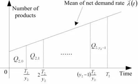
t increases over time, the production lot size may not be the same each time. Suppose that there are y2 production activities in this phase and that the lengths of time periods between production activities are the same. Once y2 is determined, the production lot sizesj
Q2, can be calculated as shown in Fig. 3 and the following:
( )
( )
(
2 1)
, 0,..., 1.2 ~ 2 2 2 2 2 2 2 2 1 , 2 2 2 2 2 − = ⎟⎟ ⎠ ⎞ ⎜⎜ ⎝ ⎛ + ⎟⎟ ⎠ ⎞ ⎜⎜ ⎝ ⎛ + = =
∫
+ y j y T b y T j a dt tQ j T y
y T j
j λ
(5)
[image:3.595.313.539.594.754.2]To choose an optimal y2, we establish the following mathematical model, in which TC2 is the sum of the fixed
Fig. 3 Relations between net demand rate and decision variables in phase 2
cost of manufacturing orders and the holding cost:
( )
( ) . ~ min 2 2 22 2 2
2 2 1 , 2 1 0 2 2
∫
∫
∑
− + = ⎟ ⎠ ⎞ ⎜ ⎝ ⎛ − + = y T j y T j t y T j j y j y dt dx x Q h fy TCλ (6)
The second term in Eq.(6) refers to the holding cost, which is the integration of the inventory level multiplied by the unit holding cost h. The inventory level function I
( )
t (safety stock not considered yet) is illustrated in Fig. 4 and the following:( )
( )
(
)
2 22 2 2 2 2 2 2 2 2 2 2 , 2 , 2 1 ; 1 ,..., 0 , 2 ~ 2 2 y T j t y T j y j y T j t b y T j t a Q dx x Q t I j t y T j j + ≤ ≤ − = ⎟⎟ ⎟ ⎠ ⎞ ⎜⎜ ⎜ ⎝ ⎛ ⎟⎟ ⎠ ⎞ ⎜⎜ ⎝ ⎛ − + ⎟ ⎟ ⎠ ⎞ ⎜ ⎜ ⎝ ⎛ ⎟⎟ ⎠ ⎞ ⎜⎜ ⎝ ⎛ − − = −
=
∫
λ(7)
Applying Eqs. (5) and (7) to Eq.(6), we obtain the following model:
. 2
4 12
min 2 2 2 23 22 2 23 2 22 21
2 ⎟⎟⎠
⎞ ⎜⎜ ⎝ ⎛ ⎟ ⎠ ⎞ ⎜ ⎝ ⎛ + + +
= fy h a T y− a T b T y−
TC
y (8)
To prove that TC2 is a convex function, we calculate the first order and the second order derivatives of TC2 in the following: ⎟⎟ ⎠ ⎞ ⎜⎜ ⎝ ⎛ ⎟ ⎠ ⎞ ⎜ ⎝ ⎛ + + −
= − −2
2 2 2 2 3 2 2 3 2 3 2 2 2 2 2 4
6 T y
b T a y T a h f dy dTC (9) ⎟⎟ ⎠ ⎞ ⎜⎜ ⎝ ⎛ ⎟ ⎠ ⎞ ⎜ ⎝ ⎛ + +
= − −3
2 2 2 2 3 2 2 4 2 3 2 2 2 2 2 2 2
2 T bT y
a y T a h dy TC d . (10) Qa2,b2,h,T2>0 and y2≥1,
∴ 0 2 2 2 2 > dy TC d
, TC2 is convex.
Therefore, we let 0
2 2 = dy dTC
to calculate the optimal y2 that minimizes TC2. It follows:
0 6 2 4 3 2 2 2 2 2 2 3 2 2 3
2 ⎟ − =
⎠ ⎞ ⎜
⎝
⎛ +
−h a T b T y a hT
fy . (11)
[image:3.595.59.281.624.760.2]Eq. (11) is a cubic equation in y2 and can be solved using Cardano formula or other suitable methods.
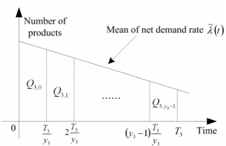
Fig. 5 Relations between net demand rate and decision variables in phase 3
However, the solution obtained from Cardano formula may not be an integer solution. Recall that TC2 is a convex function; we can calculate TC2 values of the nearest two integers to the solution obtained from Cardano formula and choose the one with smaller TC2 value as the optimal solution for y2.
The net demand of new manufactured products at time t follows normal distribution with the mean
( ) ( ) ( )
2 2~ b t a t t
t =λ −γ = +
λ and the variance σλ2+σγ2 . Therefore, the total demand for new manufactured products during the lead time of jthproduction activity in this phase also follows normal distribution with the mean
( )
2 2 2 2 2 2 2 , 2 ,..., 1 , 2 ~ 2 2 2 2 y j b a y T j a dt tD jT y
y jT j = + − = =
∫
− τ τ τ λ τ (12)and the variance τ
(
σλ2+σγ2)
. To prevent stockout, the following safety stock is necessary:(
)
(
2 2)
1
2= τσλ+σγ
−
LOS F
s . (13)
The reorder point forjthproduction activity in this phase is then derived:
(
)
(
)
, 1,..., 2. 2 2 1 , 2 2 , 2 , 2 y j LOS F D s D ROP j j j = + + = + = − γ λ σ σ τ (14)Once the inventory level is less than ROP2,j, an order for manufacturing Q2,j products is placed. Note that both the reorder point and the production lot size will increase each time due to the increasing net demand in this phase.
C. Maturity phase (phase 3)
[image:4.595.305.550.89.285.2]In this phase, the demand stops increasing and keeps in a steady state, while more and more end-of-use and end-of-life products are returned. For simplification, we suppose λ
( )
t is a constant and γ( )
t increase linearly over time in this phase. Fig. 5 illustrates the relations between the mean of net demand rate λ~( )
t and other decision variables in this phase. Suppose( )
3 3~
b t a
t = +
λ ; we can derive the production lot
sizes Q3,j and the reorder point ROP3,j following a similar procedure as in phase 2. First, Q3,j can be derived as
( )
( )
(
2 1)
, 0,..., 12 ~ 3 3 3 3 2 3 3 3 1 , 3 3 3 3 3 − = ⎟⎟ ⎠ ⎞ ⎜⎜ ⎝ ⎛ + ⎟⎟ ⎠ ⎞ ⎜⎜ ⎝ ⎛ + = =
∫
+ y j y T b y T j a dt tQ j T y
y T j
j λ
(15)
where y3 is obtained by solving the following mathematical model:
( )
( ) . ~ min 3 3 33 3 3
3 3 1 , 3 1 0 3 3
∫
∫
∑
− + = ⎟ ⎠ ⎞ ⎜ ⎝ ⎛ − + = y T j y T j t y T j j y j y dt dx x Q h fy TCλ (16)
Eq.(16) can be simplified as follow:
⎟⎟ ⎠ ⎞ ⎜⎜ ⎝ ⎛ ⎟ ⎠ ⎞ ⎜ ⎝ ⎛ + + +
= − −1
3 2 3 3 3 3 3 2 3 3 3 3 3 3 2 4 12 min 3 y T b T a y T a h fy TC
y . (17)
To prove that TC3 is a convex function, we calculate the first order and the second order derivatives of TC3 as follows: ⎟⎟ ⎠ ⎞ ⎜⎜ ⎝ ⎛ ⎟ ⎠ ⎞ ⎜ ⎝ ⎛ + + −
= − −2
3 2 3 3 3 3 3 3 3 3 3 3 3 3 2 4
6 T y
b T a y T a h f dy dTC (18)
(
) (
)
⎟ ⎠ ⎞ ⎜ ⎝ ⎛ − + + = ⎟⎟ ⎠ ⎞ ⎜⎜ ⎝ ⎛ ⎟ ⎠ ⎞ ⎜ ⎝ ⎛ + + = − − − 3 3 3 3 3 3 3 4 3 2 3 3 3 2 3 3 3 3 3 4 3 3 3 3 2 3 3 2 1 2 2 2 y b T a y T a y hT y T b T a y T a h dy TC d (19)Qa3T3+b3≥0, a3<0 and y3≥1,
∴ 2 0
3 3 2 ≥ dy TC d
, TC3 is convex.
Therefore, we let 0 3
3 =
dy dTC
to derive the optimal y3 that minimizes TC3. It follows:
0 6 2 4 3 3 3 3 2 3 3 3 3 3 3
3 ⎟ − =
⎠ ⎞ ⎜
⎝
⎛ +
−h a T b T y a hT
fy . (20)
Eq. (20) is a cubic equation in y3 and can be solved using Cardano formula. After that, we calculate TC3 values of the nearest two integers to the solution obtained from Cardano formula and choose the one with smaller TC3 value as the optimal solution fory3.
The net demand of new manufactured products at time t follows normal distribution with the mean
( ) ( ) ( )
3 3~ b t a t t
t =λ −γ = +
λ and the variance σ +λ2 σγ2 . Therefore, the total demand for new manufactured products during the lead time of jthproduction activity in this phase also follows normal distribution with the mean
( )
3 3 2 3 3 3 3 , 3 ,..., 1 , 2 ~ 3 3 3 3 y j b a y T j a dt tD jT y
y jT j = + − = =
∫
− τ τ τ λ τ (21)(
)
(
2 2)
13= τσλ+σγ
−
LOS F
s . (22)
The reorder point forjthproduction activity in this phase is then derived:
(
)
(
)
, 1,..., 3. 22 1
, 3
3 , 3 , 3
y j LOS
F D
s D ROP
j j j
= +
+ =
+ =
−
γ
λ σ
σ
τ (23)
Once the inventory level is less than ROP3,j, an order for manufacturing Q3,j products is placed. Note that both the reorder point and the production lot size will decrease each time due to the decreasing net demand in this phase.
From Eqs. (13) and (22), we can see that the safety stocks required in phase 2 and phase 3 are the same. This result shows that the safety stock is only relevant to the length of lead time, the variance of net demand and the required level of service. If all these items in different phases are the same, the safety stocks will be the same, too.
D. Decline phase
In this phase, the demand rate starts to decline. If the demand rate is still greater than the return rate, all returned products will be remanufactured; otherwise, there will be no production of new products and some of returned products will be disposed or recycled. We further discuss these two scenarios of decline phase in the following two subsections.
D.1 Decline phase I (phase 4)
In this phase, we suppose λ
( )
t is decreasing linearly but still greater than γ( )
t , which is also assumed to be a linearly increasing function over time. The net demand rate for new manufactured products is then defined as( )
4 4~
b t a
t = +
λ ,
which is also a decreasing linear function. Therefore, we can repeat the analysis procedure in Section 3.3 and derive the following results.
Production lot size:
( )
( )
(
2 1)
, 0,..., 12
~
4 4
4 4 2
4 4 4
1 , 4
4 4
4 4
− =
⎟⎟ ⎠ ⎞ ⎜⎜ ⎝ ⎛ + ⎟⎟ ⎠ ⎞ ⎜⎜ ⎝ ⎛ + =
=
∫
+y j
y T b y T j a
dt t
Q j T y
y T j
j λ
(24)
where y4 is obtained by solving the following integer cubic equation:
1 , integer
, 0 6
2 4
4 4
3 4 4 4 2 4 4 3 4 4 3 4
≥ ∈
= −
⎟ ⎠ ⎞ ⎜
⎝
⎛ +
−
y y
hT a y T b T a h fy
. (25)
Reorder point:
(
)
(
)
42 2 1
, 4 ,
4 D F LOS , j 1,...,y
ROP j= j+ + =
−
γ
λ σ
σ
τ (26)
where 4 4
2 4
4 4 4 ,
4 , 1,...,
2 b j y
a y T j a
D j = τ − τ + τ = .
D.2 Decline phase II (phase 5)
In this phase, the demand rate keeps declining and is lower than the return rate. Therefore, the excess returned products appears and some will be disposed or recycled to reduce the unnecessary remanufacturing and holding costs. In addition, all products come from remanufacturing and no new products
will be produced. As a result, there is no need to calculate the production lot size and the reorder point. However, to ensure the required level of service, we have to control the inventoryI
( )
t at the following level:( ) ( )
t λ t F(
LOS)
σλI = + −1 (27)
When a product is returned at time t, it will be remanufactured if the current inventory level is less than
( )
(
)
σλλt +F−1 LOS ; otherwise, it will be disposed or recycled.
E. Summary
From above analysis, we make some remarks in the following. Although the prediction of the phase length is usually regarded as an important issue, the production lot size
1
Q and the reorder point ROP1 in phase 1 are irrelevant to the phase length according to Eqs. (2) through (4). The prediction of the demand rate, instead, is more important in this phase (phase 1). Different from phase 1, the phase lengths in phase 2 to phase 4 will affect the inventory policies. In addition, the production lot sizes and the reorder points in phase 2 to phase 4 can be calculated using the same formula, as long as the net demand rate function λ~
( )
t is derived first.IV. NUMERICAL EXAMPLES
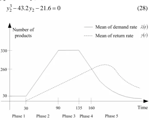
In this section, we provide a numerical example to show how the proposed method works. Fig. 6 shows the demand rate and return rate functions for the numerical example. Other parameters are given as: τ=3, f =500, h=0.1,
100 2=
λ
σ , σγ2=200 and LOS=0.97 . The inventory control policy in each phase is discussed in the following. Phase 1:
Let a1=30. The optimal production lot size, reorder point, and safety stock are derived as follows:
1
Q =547.72; ROP1=122.58; s1=32.58 Phase 2:
From Fig. 6, we have a2=3, b2=30, T2=60. First, we have to calculate the optimal number of production activities
2
y . From Eq.(11), we have 0 6 . 21 2 . 43 2 3
2− y − =
[image:5.595.307.548.559.752.2]y (28)
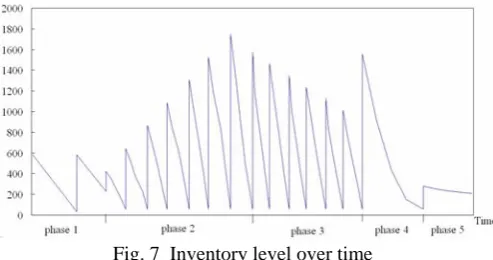
Fig. 7 Inventory level over time
Solve Eq. (28) using Cardano formula or any other capable tools, we have y2=6.809685. The integer solution will be
2
y =7, because TC2
( )
6 >TC2( )
7 . The optimal production lot size and reorder point are then derived as follows:6 ,..., 0 ,
35 . 367 41 . 220
,
2 = j+ j=
Q j (29)
7 ,..., 1 ,
92 . 132 14 . 77 ,
2 = j+ j=
ROP j . (30)
The safety stock s2=56.42. Phase 3:
Let a3=-2, b3=210, T3=45. From Eq.(20), we have
0 5 . 3037 25
. 16706
500y33− y3+ = (31)
Solve Eq. (31) and we have y3=5.687206. The integer solution will be y3 =6, because TC3
( )
5 >TC3( )
6 . The optimal production lot size and reorder point are then derived as follows:5 ,..., 0 ,
75 . 1518 5 . 112 ,
3 =− j+ j=
Q j (32)
6 ,..., 1 ,
42 . 695 45 ,
3 =− j+ j=
ROP j . (33)
The safety stock s3=56.42. Phase 4:
Let a4=-4.8, b4=120, T4=25. From Eq.(20), we have
0 5 . 2 75 .
3 4
3
4− y + =
y (34)
Solve Eq. (34) and we have y4=1.402801. The integer solution will be y4 =1, because TC4
( )
2 >TC4( )
1 . The optimal production lot size and reorder point are Q4,0=1500 and ROP4,1=78.02 , respectively. The safety stock42 . 56 4 =
s .
Phase 5:
In this phase we have to control the inventory level at:
( ) ( )
t = t +18.81I λ (35)
A returned product will be disposed or recycled if the current inventory level is higher than λ
( )
t +18.81.Under the above inventory control policy, the inventory level over time is illustrated in Fig. 7.
V. CONCLUDING REMARKS
In this paper, we have analyzed the relation between demand rate and return rate in a manufacturing/ remanufacturing system during each phase of product life-cycle. The major contribution of the paper is that the closed-form formulas of optimal production lot size, reorder point, and safety stock in each phase of product life-cycle are successfully derived. The numerical example shows the
practicability of our model and indicates that different inventory control policies should be adopted in different phases of product life-cycle. In phase 1, the EOQ model with safety stock is workable. In phase 2, the production lot size should be increased each time. On the contrary, the production lot size should be decreased each time in phase 3 and phase 4. Finally, there is no need to manufacture new products in phase 5. Some returned products are even disposed to reduce the unnecessary remanufacturing and holding costs. In phase 5 we only have to keep the inventory at a decreasing level that can ensure the required level of service.
REFERENCES
[1] S. Seuring and M. Müller, “From a literature review to a conceptual framework for sustainable supply chain management,” Journal of Cleaner Production, vol. 16, 2008, pp. 1699-1710.
[2] R. Piplani, N. Pujawan and S. Ray, “Sustainable supply chain management,” International Journal of Production Economics, vol. 111, 2007, pp. 193-194.
[3] S. Rahimifard and A.J. Clegg, “Aspects of sustainable design and manufacture,” International Journal of Production Research, vol. 45, 2007, pp. 4013-4019.
[4] S. Seuring, J. Sarkis, M. Müller and P. Rao, “Sustainability and supply chain management - An introduction to the special issue,” Journal of Cleaner Production, vol. 16, 2008, pp. 1545-1551.
[5] V. Jayaram, R. Klassen and J.D. Linton, “Supply chain management in a sustainable environment,” Journal of Operations Management vol. 25, 2007, pp. 1071-1074.
[6] S.K. Srivastava, “Green supply-chain management: A state-of-the-art literature review,” International Journal of Management Reviews, vol. 9, 2007, pp. 53-80.
[7] J. Östlin, E. Sundin and M. Björkman, “Importance of closed-loop supply chain relationships for product remanufacturing,” International Journal of Production Economics, vol. 115, 2008, pp. 336-348. [8] E. Van der Laan, R. Dekker and M. Salomon, “Product
remanufacturing and disposal: A numerical comparison of alternative control strategies,” International Journal of Production Economics, vol. 45, 1996, pp. 489-498.
[9] E. van der Laan and M. Salomon, “Production planning and inventory control with remanufacturing and disposal,” European Journal of Operational Research, vol. 102, 1997, pp. 264-278.
[10] E. van der Laan, M. Salomon, R. Dekker and L. van Wasserihove, “Inventory control in hybrid systems with remanufacturing,”
Management Science, 1999, vol. 45, pp. 733-747.
[11] E. van der Laan, M. Salomon and R. Dekker, “An investigation of lead-time effects in manufacturing/remanufacturing systems under simple PUSH and PULL control strategies,” European Journal of Operational Research, vol. 115,1999, pp.195-214.
[12] G.P. Kiesmüller, “Optimal control of a one product recovery system with leadtimes,” International Journal of Production Economics, vol. 81-82, 2003, pp. 333-340.
[13] H. Ouyang and X. Zhu, “An inventory control model with disposal for manufacturing/remanufacturing hybrid system,” Computers & Industrial Engineering, 2008, doi:10.1016/j.cie.2008.07.008
[14] S.K. Mukhopadhyay and H. Ma, “Joint procurement and production decisions in remanufacturing under quality and demand uncertainty,”
International Journal of Production Economics, vol. 120, 2009, pp.5-17.
[15] G.P. Kiesmüller and E. van der Laan, “An inventory model with dependent product demands and returns,” International Journal of Production Economics, vol. 72, 2001, pp. 73-87.
[16] I. Dobos, “Optimal production–inventory strategies for a HMMS-type reverse logistics system,” International Journal of Production Economics, vol. 81-82, 2003, pp. 351-360.