A Fast Boosting-based Learner for Feature-Rich Tagging and Chunking
Tomoya Iwakura Seishi Okamoto
Fujitsu Laboratories Ltd.
1-1, Kamikodanaka 4-chome, Nakahara-ku, Kawasaki 211-8588, Japan {iwakura.tomoya,seishi}@jp.fujitsu.com
Abstract
Combination of features contributes to a significant improvement in accuracy on tasks such as part-of-speech (POS) tag-ging and text chunking, compared with us-ing atomic features. However, selectus-ing combination of features on learning with large-scale and feature-rich training data requires long training time. We propose a fast boosting-based algorithm for learning rules represented by combination of fea-tures. Our algorithm constructs a set of rules by repeating the process to select sev-eral rules from a small proportion of can-didate rules. The cancan-didate rules are gen-erated from a subset of all the features with a technique similar to beam search. Then we propose POS tagging and text chunk-ing based on our learnchunk-ing algorithm. Our tagger and chunker use candidate POS tags or chunk tags of each word collected from automatically tagged data. We evaluate our methods with English POS tagging and text chunking. The experimental results show that the training time of our algo-rithm are about 50 times faster than Sup-port Vector Machines with polynomial ker-nel on the average while maintaining state-of-the-art accuracy and faster classification speed.
1 Introduction
Several boosting-based learning algorithms have been applied to Natural Language Processing problems successfully. These include text catego-rization (Schapire and Singer, 2000), Natural Lan-guage Parsing (Collins and Koo, 2005), English syntactic chunking (Kudo et al., 2005) and so on.
c
°2008. Licensed under the Creative Commons Attribution-Noncommercial-Share Alike 3.0 Unported li-cense (http://creativecommons.org/licenses/by-nc-sa/3.0/). Some rights reserved.
Furthermore, classifiers based on boosting-based learners have shown fast classification speed (Kudo et al., 2005).
However, boosting-based learning algorithms require long training time. One of the reasons is that boosting is a method to create a final hypoth-esis by repeatedly generating a weak hypothhypoth-esis in each training iteration with a given weak learner. These weak hypotheses are combined as the fi-nal hypothesis. Furthermore, the training speed of boosting-based algorithms becomes more of a problem when considering combination of features that contributes to improvement in accuracy.
This paper proposes a fast boosting-based algo-rithm for learning rules represented by combina-tion of features. Our learning algorithm uses the following methods to learn rules from large-scale training samples in a short time while maintaining accuracy; 1) Using a rule learner that learns sev-eral rules as our weak learner while ensuring a re-duction in the theoretical upper bound of the train-ing error of a boosttrain-ing algorithm, 2) Repeattrain-ing to learn rules from a small proportion of candidate rules that are generated from a subset of all the fea-tures with a technique similar to beam search, 3) Changing subsets of features used by weak learner dynamically for alleviating overfitting.
We also propose feature-rich POS tagging and text chunking based on our learning algorithm. Our POS tagger and text chunker use candidate tags of each word obtained from automatically tagged data as features.
The experimental results with English POS tag-ging and text chunking show drastically improve-ment of training speeds while maintaining compet-itive accuracy compared with previous best results and fast classification speeds.
2 Boosting-based Learner
2.1 Preliminaries
We describe the problem treated by our boosting-based learner as follows. LetX be the set of ex-amples and Y be a set of labels {−1,+1}. Let
F = {f1, f2, ..., fM}beM types of features rep-resented by strings. LetSbe a set of training
##S={(xi, yi)}mi=1:xi⊆ X,yi∈ {±1}
## a smoothing valueε=1
## rule number r: the initial value is 1.
Initialize: Fori=1,...,m:w1,i=exp(12log(WW+1−1)); While(r≤R)
## Train weak-learner using (S,{wr,i}mi=1)
## Getνtypes of rules:{fj}νj=1
{fj}νj=1←weak-learner(S,{wr,i}mi=1);
## Update weights with confidence value Foreachf∈ {fj}νj=1
c= 1
2log(WWr,r,−+11((ff)+)+εε)
Fori=1,...,m: wr+1,i=wr,iexp(−yihhf,ci)
fr=f;cr =c;r++; endForeach
endWhile
Output:F(x) =sign(log(W+1
W−1) +
PR
r=1hhfr,cri(x))
Figure 1: A generalized version of our learner ples{(x1, y1), ...,(xm, ym)}, where each example
xi ∈ X consists of features inF, which we call a feature-set, andyi ∈ Yis a class label. The goal is to induce a mapping
F :X → Y
fromS.
Let|xi|(0<|xi| ≤M)be the number of fea-tures included in a feature-set xi, which we call the size ofxi, andxi,j ∈ F (1 ≤ j ≤ |xi|) be a feature included in xi. 1 We call a feature-set of size ka k-feature-set. Then we define subsets of feature-sets as follows.
Definition 1 Subsets of feature-sets
If a feature-setxj contains all the features in a
feature-setxi, then we callxiis a subset ofxjand
denote it as
xi⊆xj.
Then we define weak hypothesis based on the idea of the real-valued predictions and abstaining (RVPA, for short) (Schapire and Singer, 2000).2
Definition 2 Weak hypothesis for feature-sets
Let f be a feature-set, called a rule, x be a feature-set, andc be a real number, called a con-fidence value, then a weak-hypothesis for feature-sets is defined as
hhf,ci(x) =
½
c f⊆x
0 otherwise.
1Our learner can handle binary vectors as in (Morishita,
2002). When our learner treats binary vectors forMattributes {X1,...,Xm}, the learner converts each vector to the
corre-sponding feature-set asxi ← {fi|Xi,j ∈ Xi∧Xi,j = 1}
(1≤i≤m,1≤j≤M).
2We use the RVPA because training with RVPA is faster
than training with Real-valued-predictions (RVP) while main-taining competitive accuracy (Schapire and Singer, 2000). The idea of RVP is to output a confidence value for samples which do not satisfy the given condition too.
2.2 Boosting-based Rule Learning
Our boosting-based learner selectsRtypes of rules for creating a final hypothesisFon several training iterations. TheFis defined as
F(x) =sign(PR
r=1hhfr,cri(x)).
We use a learning algorithm that generates several rules from a given training samples
S = {(xi, yi)}mi=1 and weights over samples
{wr,1, ..., wr,m}as input of our weak learner. wr,i is the weight of sample number i after selecting
r−1types of rules, where0<wr,i,1≤i≤mand
1≤r≤R.
Given such input, the weak learner selects ν
types of rules{fj}νj=1(fj ⊆ F)withgain:
gain(f) def= |pW
r,+1(f)−
p
Wr,−1(f)|,
wherefis a feature-set, and Wr,y(f)is
Wr,y(f) =Pmi=1wr,i[[f⊆xi∧yi=y]], and[[π]]is 1 if a propositionπ holds and 0 other-wise.
The weak learner selects a feature-set having the highestgainas the first rule, and the weak learner finally selectsν types of feature-sets havinggain
in topνas{fj}νj=1at each boosting iteration. Then the boosting-based learner calculates the confidence value of eachf in{fj}νj=1 and updates the weight of each sample. The confidence value
cj forfjis defined as
cj=12log(WWr,r,+1−1((ffjj))).
After the calculation ofcj for fj, the learner up-dates the weight of each sample with
wr+1,i = wr,iexp(−yihhfj,cji). (1)
Then the learner adds (fj, cj) to F as the r -th rule and its confidence value. 3 When we calculate the confidence value cj+1 for fj+1, we use{wr+1,1, ..., wr+1,m}. The learner adds (fj+1,
cj+1) toFas ther+1-th rule and confidence value. After the updates of weights with {fj}νj=1, the learner starts the next boosting iteration. The learner continues training until obtainingRrules.
Our boosting-based algorithm differs from the other boosting algorithms in the number of rules learned at each iteration. The other boosting-based algorithms usually learn a rule at each iteration 3Eq. (1) is the update of the AdaBoost used in ADTrees
##sortByW(F,fq): Sort features (f∈ F) ## in ascending order based on weights of features ##(a%b): Return the reminder of(a÷b) ##|B|-buckets:B={B[0], ..., B[|B| −1]}
proceduredistFT(S,|B|)
##Calculate the weight of each feature
Foreach(f∈F) Wr(f) =Pmi=1wr,i[[{f} ⊆xi]]
##Sort features based on thier weights and ## store the results inF s
F s←sortByW(F, Wr)
## Distribute features to buckets
Fori=0...M: B[(i%|B|)] = (B[(i%|B|)]∪F s[i]) returnB
Figure 2: Distribute features to buckets based on weights
(Schapire and Singer, 2000; Freund and Mason, 1999). Despite the difference, our boosting-based algorithm ensures a reduction in the theoretical up-per bound of training error of the AdaBoost. We list the detailed explanation in Appendix.A.
Figure 1 shows an overview of our boosting-based rule learner. To avoid to happen that
Wr,+1(f) orWr,−1(f) is very small or even zero, we use the smoothed values ε (Schapire and Singer, 1999). Furthermore, to reflect imbalance class distribution, we use the default rule (Freund and Mason, 1999), defined as 1
2log(WW+1−1), where Wy = Pmi=1[[yi = y]]for y ∈ {±1}. The initial weights are defined with the default rule.
3 Fast Rule Learner
3.1 Generating Candidate Rules
We use a method to generate candidate rules with-out duplication (Iwakura and Okamoto, 2007). We denotef0=f+f as the generation ofk+ 1 -feature-set f0 consisting of a feature f and a k -feature-set f. Let ID(f) be the integer corre-sponding to f, called id, and φbe 0-feature-set. Then we definegengenerating a feature-set as
gen(f, f) =
(
f+f if ID(f)>max f0∈f ID(f
0)
φ otherwise .
We assign smaller integer to more infrequent fea-tures as id. If there are features having the same frequency, we assign idto each feature with lexi-cographic order of features. Training based on this candidate generation showed faster training speed than generating candidates by an arbitrary order (Iwakura and Okamoto, 2007).
3.2 Training with Redistributed Features We propose a method for learning rules by repeat-ing to select a rule from a small portion of can-didate rules. We evaluated the effectiveness of four types of methods to learn a rule from a sub-set of features on boosting-based learners with a text chunking task (Iwakura and Okamoto, 2007). The results showed that Frequency-based distribu-tion (F-dist) has shown the best accuracy. F-dist
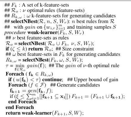
##Fk: A set of k-feature-sets
##Ro:νoptimal rules (feature-sets)
##Rk,ω:ωk-feature-sets for generating candidates
##selectNBest(R,n,S,Wr):nbest rules fromR
## withgainon{wi,r}mi=1and training samplesS procedureweak-learner(Fk,S,Wr)
##νbest feature-sets as rules
Ro=selectNBest(Ro∪Fk, ν,S,Wr); if(ζ≤k)returnRo; ## Size constraint
##ωbest feature-sets inFkfor generating candidates
Rk,ω=selectNBest(Fk,ω,S,Wr);
τ=min
f∈Rogain(f); ## Thegainofν-th optimal rule Foreach(fk∈Rk,ω)
if(u(fk)< τ)continue; ## Upper bound of gain
Foreach(f∈ F) ## Generate candidates
fk+1=gen(fk, f);
if (ξ≤Pm
i=1[[fk+1⊆xi]])Fk+1= (Fk+1∪fk+1);
end Foreach end Foreach
[image:3.595.310.530.72.268.2]return weak-learner(Fk+1, S, W);
Figure 3: Find optimal feature-sets with given weights
distributes features to subsets of features, called buckets, based on frequencies of features.
However, we guess training using a subset of features depends on how to distribute features to buckets like online learning algorithms that gener-ally depend on the order of the training examples (Kazama and Torisawa, 2007).
To alleviate the dependency on selected buck-ets, we propose a method that redistributes fea-tures, called Weight-based distribution (W-dist).
W-dist redistributes features to buckets based on the weight of feature defined as
Wr(f) =Pmi=1wr,i[[{f} ⊆xi]]
for eachf ∈ F after examining all buckets. Fig-ure 2 describes an overview ofW-dist.
3.3 Weak Learner for Learning Several Rules We propose a weak learner that learns several rules from a small portion of candidate rules.
Figure 3 describes an overview of the weak learner. At each iteration, one of the|B|-buckets is given as an initial 1-feature-setsF1. The weak learner findsν best feature-sets as rules from can-didates consisting ofF1and feature-sets generated fromF1. The weak learner generates candidatesk -feature-sets (1< k) fromωbest (k-1)-feature-sets inFk−1withgain.
We also use the following pruning techniques (Morishita, 2002; Kudo et al., 2005).
•Frequency constraint: We examine candidates
seen on at leastξdifferent examples.
•Size constraint: We examine candidates whose
size is no greater than a size thresholdζ.
•Upper bound of gain: We use the upper bound
of gain defined as
u(f)def=max(pW
r,+1(f),pWr,−1(f)).
For any feature-setf0⊆F, which contains f (i.e.
f ⊆f0), thegain(f0)is bounded underu(f), since
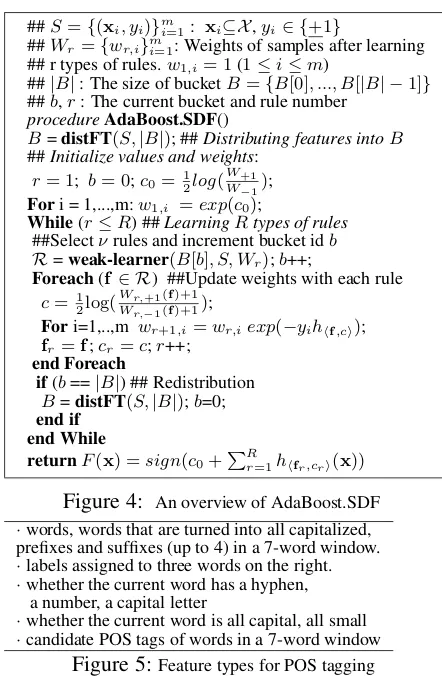
##S={(xi, yi)}mi=1: xi⊆X,yi∈ {+1}
##Wr ={wr,i}mi=1: Weights of samples after learning
## r types of rules.w1,i= 1(1≤i≤m)
##|B|: The size of bucketB={B[0], ..., B[|B| −1]} ##b,r: The current bucket and rule number
procedureAdaBoost.SDF()
B=distFT(S,|B|); ##Distributing features intoB ##Initialize values and weights:
r= 1; b= 0;c0=21log(WW+1−1);
Fori = 1,...,m:w1,i =exp(c0);
While(r≤R) ##LearningRtypes of rules
##Selectνrules and increment bucket idb R=weak-learner(B[b], S, Wr);b++;
Foreach(f ∈ R) ##Update weights with each rule c=1
2log(WWr,r,+1−1((ff)+1)+1);
Fori=1,..,m wr+1,i=wr,iexp(−yihhf,ci);
fr=f;cr=c;r++; end Foreach
if(b==|B|) ## Redistribution B=distFT(S,|B|);b=0; end if
end While
[image:4.595.70.291.67.405.2]returnF(x) =sign(c0+PRr=1hhfr,cri(x))
Figure 4: An overview of AdaBoost.SDF ·words, words that are turned into all capitalized, prefixes and suffixes (up to 4) in a 7-word window. ·labels assigned to three words on the right. ·whether the current word has a hyphen,
a number, a capital letter
·whether the current word is all capital, all small ·candidate POS tags of words in a 7-word window
Figure 5:Feature types for POS tagging
is less than thegainof the current optimal ruleτ, candidates containingfare safely pruned.
Figure 4 describes an overview of our algorithm, which we call AdaBoost for a weak learner learn-ing Several rules from Distributed Features ( Ad-aBoost.SDF, for short).
The training of AdaBoost.SDF with (ν = 1, ω =∞,1<|B|) is equivalent to the approach of AdaBoost.DF (Iwakura and Okamoto, 2007). If we use (|B|= 1,ν = 1), AdaBoost.SDF examines all features on every iteration like (Freund and Ma-son, 1999; Schapire and Singer, 2000).
4 POS tagging and Text Chunking
4.1 English POS Tagging
We used the Penn Wall Street Journal treebank (Marcus et al., 1994). We split the treebank into training (sections 0-18), development (sections 19-21) and test (sections 22-24) as in (Collins, 2002). We used the following candidate POS tags, called candidate feature, in addition to commonly used features (Gim´enez and M`arquez, 2003; Toutanova et al., 2003) shown in Figure 5.
We collect candidate POS tags of each word from the automatically tagged corpus provided for the shared task of English Named Entity recog-nition in CoNLL 2003. 4 The corpus includes 17,003,926 words with POS tags and chunk tags
4http://www.cnts.ua.ac.be/conll2003/ner/
·words and POS tags in a 5-word window. ·labels assigned to two words on the right.
·candidate chunk tags of words in a 5-word window
Figure 6:Feature types for text chunking
annotated by a POS tagger and a text chunker. Thus, the corpus includes wrong POS tags and chunk tags.
We collected candidate POS tags of words that appear more than 9 times in the corpus. We express these candidates with one of the following ranges decided by their frequencyfq; 10 ≤ fq < 100,
100≤fq <1000and1000≤fq.
For example, we express ’work’ annotated as NN 2000 times like “1000≤NN”. If ’work’ is cur-rent word, we add1000≤NN as a candidate POS tag feature of the current word. If ’work’ appears the next of the current word, we add1000≤NN as a candidate POS tag of the next word.
4.2 Text Chunking
We used the data prepared for CoNLL-2000 shared tasks. 5 This task aims to identify 10 types of chunks, such as, NP, VP and PP, and so on.
The data consists of subsets of Penn Wall Street Journal treebank; training (sections 15-18) and test (section 20). We prepared the development set from section 21 of the treebank as in (Tsuruoka and Tsujii, 2005).6
Each base phrase consists of one word or more. To identify word chunks, we useIOE2 representa-tion. The chunks are represented by the following tags: E-X is used for end word of a chunk of class X. I-X is used for non-end word in an X chunk. O is used for word outside of any chunk.
For instance, “[He] (NP) [reckons] (VP) [the current account deficit] (NP)...” is represented by IOE2 as follows; “He/E-NP reckons/E-VP the/I-NP current/I-the/I-NP account/I-the/I-NP deficit/E-the/I-NP”.
We used features shown in Figure 6. We col-lected the followings as candidate chunk tags from the same automatically tagged corpus used in POS tagging.
• Candidate tags expressed with frequency infor-mation as in POS tagging
• The ranking of each candidate decided by fre-quencies in the automatically tagged data
• Candidate tags of each word
For example, if we collect “work” anno-tated as I-NP 2000 times and as E-VP 100 time, we generate the following candidate fea-tures for “work”; 1000≤I-NP,100≤E-VP<1000, rank:I-NP=1 rank:E-NP=2, candidate=I-NP and candidate=E-VP.
5http://lcg-www.uia.ac.be/conll2000/chunking/ 6We usedhttp://ilk.uvt.nl/˜sabine/chunklink/chunklink 2-2-2000 for conll.pl
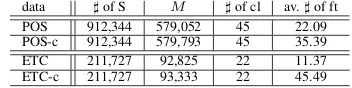
Table 1: Training data for experiments: ]of S,M,] of cl and av. ]of ft indicate the number samples, the distinct number of feature types, the number of class in each data set, and the average number of features, respectively. POS and ETC indicate POS-tagging and text chunking. The “-c” in-dicates using candidate features collected from parsed unla-beled data.
data ]of S M ]of cl av.]of ft
POS 912,344 579,052 45 22.09
POS-c 912,344 579,793 45 35.39
ETC 211,727 92,825 22 11.37
ETC-c 211,727 93,333 22 45.49
We converted the chunk representation of the automatically tagged corpus to IOE2 and we col-lected chunk tags of each word appearing more than nine times.
4.3 Applying AdaBoost.SDF
AdaBoost.SDF treats the binary classification problem. To extend AdaBoost.SDF to multi-class, we used the one-vs-the-rest method.
To identify proper tag sequences, we use Viterbi search. We map the confidence value of each clas-sifier into the range of 0 to 1 with sigmoid function 7, and select a tag sequence which maximizes the sum of those log values by Viterbi search.
5 Experiments
5.1 Experimental Settings
We compared AdaBoost.SDF with Support Vec-tor Machines (SVM). SVM has shown good per-formance on POS tagging (Gim´enez and M`arquez, 2003) and Text Chunking (Kudo and Matsumoto, 2001). Furthermore, SVM with polynomial kernel implicitly expands all feature combinations with-out increasing the computational costs. Thus, we compared AdaBoost.SDF with SVM.8
To evaluate the effectiveness of candidate fea-tures, we examined two types of experiments with candidate features and without them. We list the statics of training sets in Table 1.
We tested R=100,000, |B|=1,000, ν =
{1,10,100}, ω={1,10,100,∞}, ζ={1,2,3}, and
ξ={1,5} for AdaBoost.SDF. We tested the soft margin parameter C={0.1,1,10} and the kernel degreed={1,2,3}for SVM.9
We used the followings for comparison; Train-ing timeis time to learn 100,000 rules. Best train-ing time is time for generating rules to show the best F-measure (Fβ=1) on development data.
Ac-curacyisFβ=1on a test data with the rules atbest
training time.
7s(X) = 1/(1 +exp(−βX)), where X = F(x)is a
output of a classifier. We usedβ=5 in this experiment.
8We used TinySVM(http://chasen.org/˜taku/software/TinySVM/). 9We used machines with 2.66 GHz QuadCore Intel Xeon
and 10 GB of memory for all the experiments.
Table 2: Experimental results of POS tagging and Text Chunking (TC) with candidate features. F and time indicate the averageFβ=1of test data and time (hour) to learn 100,000
rules for all classes withF-dist. These results are listed sepa-rately with respect to eachξ={1,5}.
ν POS(ξ= 1) POS (ξ= 5) TC (ξ= 1) TC (ξ= 5)
F time F time F time F time
1 97.27 196.3 97.23 195.7 93.98 145.3 93.95 155.8
10 97.23 23.05 97.17 22.35 93.96 2.69 93.88 2.70
100 96.82 2.99 96.83 2.91 93.16 0.74 93.14 0.56
88 89 90 91 92 93 94
0 2 4 6 8 10
Accuracy (F-measure)
Training Time (hour)
ζ=3 ω=∞ ν=1 ζ=3 ω=∞ ν=10 ζ=3 ω=∞ ν=100 ζ=3 ω=1 ν=1 ζ=3 ω=1 ν=10 ζ=3 ω=1 ν=100 ζ=3 ω=10 ν=1 ζ=3 ω=10ν=10 ζ=3 ω=10 ν=100 ζ=3 ω=100 ν=1 ζ=3 ω=100 ν=10 ζ=3 ω=100 ν=100
Figure 7: Accuracy on development data of Text Chunk-ing (ζ= 3) obtained with parsers based onF-dist. We mea-sured accuracy obtained with rules at each training time. The widest line is AdaBoost.SDF (ν=1,ω=∞). The others are
Ad-aBoost.SDF (ν=10(◦),ν=100(•),ν=1&ω={1,10,100}). 5.2 Effectiveness of Several Rule Learning
Table 2 shows average accuracy and training time. We usedF-dist as the distribution method. These average accuracy obtained with rules learned by AdaBoost.SDF (ν=10) on both tasks are competi-tive with the average accuracy obtained with rules learned by AdaBoost.SDF (ν=1). These results have shown that learning several rules at each iter-ation contributes significant improvement of train-ing time. These results have also shown that the learning several rule at each iteration methods are more efficient than training by just using the fre-quency constraintξ.
Figure 7 shows a snapshot for accuracy ob-tained with chunkers using different number of rules. This graph shows that chunkers based on AdaBoost.SDF (ν=10,100) and AdaBoost.SDF (ν=1,ω={1,10,100}) have shown better accuracy than chunkers based on AdaBoost.SDF (ν=1,ω=∞) at each training time. These result have shown that learning several rules at each iteration and learning combination of features as rules with a technique similar to beam search are effective in improving training time while giving a better convergence.
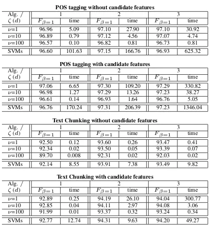
[image:5.595.92.268.143.187.2]Table 3: Experimental results on POS tagging and Text Chunking. Accuracies(Fβ=1) on test data and training time
(hour) of AdaBoost.SDF are averages ofω={1,10,100,∞}for eachζwithF-distandξ= 1.Fβ=1and time (hour) of SVMs
are averages ofC={0.1,1,10}for each kernel parameterd.
POS tagging without candidate features
Alg./ 1 2 3
ζ(d) Fβ=1 time Fβ=1 time Fβ=1 time
ν=1 96.96 5.09 97.10 27.90 97.10 30.92
ν=10 96.89 0.79 97.12 4.56 97.07 4.74
ν=100 96.57 0.10 96.82 0.81 96.73 0.81
SVMs 96.60 101.63 97.15 166.76 96.93 625.32
POS tagging with candidate features
Alg./ 1 2 3
ζ(d) Fβ=1 time Fβ=1 time Fβ=1 time
ν=1 97.06 6.65 97.30 109.20 97.29 330.82
ν=10 96.98 1.27 97.29 13.26 97.23 38.27
ν=100 96.61 0.14 96.93 1.64 96.76 5.05
SVMs 96.76 170.24 97.31 206.39 97.23 1346.04
Text Chunking without candidate features
Alg./ 1 2 3
ζ(d) Fβ=1 time Fβ=1 time Fβ=1 time
ν=1 92.50 0.12 93.60 0.26 93.47 0.41
ν=10 92.34 0.02 93.50 0.05 93.39 0.07
ν=100 89.70 0.008 92.31 0.02 92.03 0.02
SVMs 92.14 8.55 93.91 7.38 93.49 9.82
Text Chunking with candidate features
Alg./ 1 2 3
ζ(d) Fβ=1 time Fβ=1 time Fβ=1 time
ν=1 92.89 0.25 94.19 26.10 94.04 300.77
ν=10 92.85 0.04 94.11 2.97 94.08 3.06
ν=100 91.99 0.01 93.37 0.32 93.24 0.34
SVMs 92.77 12.74 94.31 9.63 94.20 49.27
5.3 Comparison with SVM
Table 3 lists average accuracy and training time on POS tagging and text chunking with respect to each (ν, ζ) for AdaBoost.SDF anddfor SVM. AdaBoost.SDF with ν=10 and ν=100 have shown much faster training speeds than SVM and Ad-aBoost.SDF ( ν=1,ω=∞) that is equivalent to the AdaBoost.DF (Iwakura and Okamoto, 2007).
Furthermore, the accuracy of taggers and chun-kers based on AdaBoost.SDF (ν=10) have shown competitive accuracy with those of SVM-based and AdaBoost.DF-based taggers and chunkers. AdaBoost.SDF (ν=10) showed about 6 and 54 times faster training speeds than those of Ad-aBoost.DF on the average in POS tagging and text chunking. AdaBoost.SDF (ν=10) showed about 147 and 9 times faster training speeds than the training speeds of SVM on the average of POS tagging and text chunking. On the average of the both tasks, AdaBoost.SDF (ν=10) showed about 25 and 50 times faster training speed than Ad-aBoost.DF and SVM. These results have shown that AdaBoost.SDF with a moderate parameter ν
can improve training time drastically while main-taining accuracy.
These results in Table 3 have also shown that rules represented by combination of features and the candidate features collected from automati-cally tagged data contribute to improved accuracy. 5.4 Effectiveness of Redistribution
We compared Fβ=1 andbest training time of
[image:6.595.306.532.123.304.2]F-dist andW-dist. We used ζ = 2that has shown
Table 4: Results obtained with taggers and chunkers based onF-dist andW-dist. These results obtained with taggers and chunkers trained withω = {1,10,100,∞}andζ = 2. F and time indicate averageFβ=1on test data and averagebest training time.
POS tagging withF-dist
ν ω=1 ω=10 ω=100 ω=∞
F time F time F time F time
1 97.31 30.03 97.31 64.25 97.32 142.9 97.26 89.59
10 97.26 3.21 97.32 9.57 97.30 15.54 97.30 19.64
100 96.86 0.62 96.95 1.32 96.95 2.13 96.96 2.43
POS tagging withW-dist
ν ω=1 ω=10 ω=100 ω=∞
F time F time F time F time
1 97.32 29.96 97.31 57.05 97.31 163.2 97.32 98.71
10 97.24 2.66 97.30 25.70 97.28 16.20 97.29 20.49
100 97.00 0.54 97.02 1.31 97.07 2.22 97.08 2.58
Text Chunking withF-dist
ν ω=1 ω=10 ω=100 ω=∞
F time F time F time F time
1 93.95 7.42 94.30 23.30 94.22 34.74 94.31 21.26
10 93.99 0.98 94.08 2.44 94.19 3.11 94.18 3.18
100 93.32 0.16 93.33 0.32 93.42 0.40 93.42 0.40
Text Chunking withW-dist
ν ω=1 ω=10 ω=100 ω=∞
F time F time F time F time
1 93.99 2.93 94.24 24.77 94.32 35.72 94.32 35.61
10 93.98 0.71 94.30 2.82 94.29 3.60 94.30 4.05
100 93.66 0.17 93.65 0.36 93.50 0.42 93.50 0.42
better average accuracy than ζ = {1,3} in both tasks. Table 4 lists comparison of F-dist and W-diston POS tagging and text chunking. Most of accuracy obtained with W-dist-based taggers and parsers better than accuracy obtained withF-dist -based taggers and parsers. These results have shown thatW-distimproves accuracy without dras-tically increasing training time. The text chunker and the tagger trained with AdaBoost.SDF (ν= 10, ω = 10 and W-dist) has shown competitive
accu-racy with that of the chunker trained with Ad-aBoost.SDF (ν= 1,ω=∞andF-dist) while main-taining about 7.5 times faster training speed. 5.5 Tagging and Chunking Speeds
We measured testing speeds of taggers and chun-kers based on rules or models listed in Table 5.10
We examined two types of fast classification al-gorithms for polynomial kernel: Polynomial Ker-nel Inverted (PKI) and Polynomial KerKer-nel Ex-panded (PKE). The PKI leads to about 2 to 12 times improvements, and the PKE leads to 30 to 300 compared with normal classification approach of SVM (Kudo and Matsumoto, 2003).11
The POS-taggers based on AdaBoost.SDF, SVM with PKI, and SVM with PKE processed 4,052 words, 159 words, and 1,676 words per sec-ond, respectively. The chunkers based on these three methods processed 2,732 words, 113 words, and 1,718 words per second, respectively.
10We list average speeds of three times tests measured with
a machine with Xeon 3.8 GHz CPU and 4 GB of memory.
11We use a chunker YamCha for evaluating classification
speeds based on PKI or PKE (http://www.chasen.org/˜taku/software/
yamcha/). We list the average speeds of SVM-based tagger and
Table 5: Comparison with previous best results: (Top : POS tagging, Bottom: Text Chunking )
POS tagging Fβ=1
Perceptron (Collins, 2002) 97.11
Dep. Networks (Toutanova et al., 2003) 97.24
SVM (Gim´enez and M`arquez, 2003) 97.05
ME based a bidirectional inference (Tsuruoka and Tsujii, 2005) 97.15
Guided learning for bidirectional sequence classification (Shen et al., 2007) 97.33
AdaBoost.SDF with candidate features(ζ=2,ν=1,ω=100,W-dist) 97.32
AdaBoost.SDF with candidate features(ζ=2,ν=10,ω=10,F-dist) 97.32
SVM with candidate features (C=0.1,d=2) 97.32
Text Chunking Fβ=1
Regularized Winnow + full parser output (Zhang et al., 2001) 94.17
SVM-voting (Kudo and Matsumoto, 2001) 93.91
ASO + unlabeled data (Ando and Zhang, 2005) 94.39
CRF+Reranking(Kudo et al., 2005) 94.12
ME based a bidirectional inference (Tsuruoka and Tsujii, 2005) 93.70
LaSo (Approximate Large Margin Update) (Daum´e III and Marcu, 2005) 94.4
HySOL (Suzuki et al., 2007) 94.36
AdaBoost.SDFwith candidate featuers (ζ=2,ν=1,ω=∞,W-dist) 94.32
AdaBoost.SDFwith candidate featuers (ζ=2,ν=10,ω=10,W-dist) 94.30
SVM with candidate features (C=1,d=2) 94.31
One of the reasons that boosting-based classi-fiers realize faster classification speed is sparseness of rules. SVM learns a final hypothesis as a linear combination of the training examples using some coefficients. In contrast, this boosting-based rule learner learns a final hypothesis that is a subset of candidate rules (Kudo and Matsumoto, 2004).
6 Related Works
6.1 Comparison with Previous Best Results We list previous best results on English POS tag-ging and Text chunking in Table 5. These results obtained with the taggers and chunkers based on AdaBoost.SDF and SVM showed competitive F-measure with previous best results. These show that candidate features contribute to create state-of-the-art taggers and chunkers.
These results have also shown that
AdaBoost.SDF-based taggers and chunkers show competitive accuracy by learning combi-nation of features automatically. Most of these previous works manually selected combination of features except for SVM with polynomial kernel and (Kudo and Matsumoto, 2001) a boosting-based re-ranking (Kudo et al., 2005). 6.2 Comparison with Boosting-based
Learners
LazyBoosting randomly selects a small proportion of features and selects a rule represented by a fea-ture from the selected feafea-tures at each iteration (Escudero et al., 2000).
Collins and Koo proposed a method only up-dates values of features co-occurring with a rule feature on examples at each iteration (Collins and Koo, 2005).
Kudo et al. proposed to perform several pseudo iterations for converging fast (Kudo et al., 2005) with features in the cache that maintains the fea-tures explored in the previous iterations.
AdaBoost.MHKRlearns a weak-hypothesis rep-resented by a set of rules at each boosting iteration
(Sebastiani et al., 2000).
AdaBoost.SDF differs from previous works in the followings. AdaBoost.SDF learns several rules at each boosting iteration like AdaBoost.MHKR. However, the confidence value of each hypothe-sis in AdaBoost.MHKRdoes not always minimize the upper bound of training error for AdaBoost because the value of each hypothesis consists of the sum of the confidence value of each rule. Compared with AdaBoost.MHKR, AdaBoost.SDF computes the confidence value of each rule to min-imize the upper bound of training error on given weights of samples at each update.
Furthermore, AdaBoost.SDF learns several rules represented by combination of features from limited search spaces at each boosting itera-tion. The creation of subsets of features in Ad-aBoost.SDF enables us to recreate the same classi-fier with same parameters and training data. Recre-ation is not ensured in the random selection of sub-sets in LazyBoosting.
7 Conclusion
We have proposed a fast boosting-based learner, which we call AdaBoost.SDF. AdaBoost.SDF re-peats to learn several rules represented by combi-nation of features from a small proportion of can-didate rules. We have also proposed methods to use candidate POS tags and chunk tags of each word obtained from automatically tagged data as features in POS tagging and text chunking.
The experimental results have shown drastically improvement of training speed while maintaining competitive accuracy compared with previous best results.
Future work should examine our approach on several tasks. Future work should also compare our algorithm with other learning algorithms.
Appendix A: Convergence
The upper bound of the training error for AdaBoost of (Freund and Mason, 1999), which is used in Ad-aBoost.SDF, is induced by adopting THEOREM 1 presented in (Schapire and Singer, 1999). LetZR be Pmi=1wR+1,i that is a sum of weights updated withRrules. The bound holds on the training er-ror after selectingRrules,
Pm
i=1[[F(xi)6=yi]]≤ZR is induced as follows.
By unraveling the Eq. (1), we obtain
wR+1,i=exp(−yiPrR=1hhfr,cri(xi)). Thus, we obtain [[F(xi) 6= yi]] ≤ exp(−yiPRt=1hhfr,cri(xi)),
m X
i=1
[[F(xi)6=yi]] ≤ m X
i=1
exp(−yi R X
t=1
hhfr,cri(xi))
= Xm i=1
wR+1,i=ZR. (2)
Then we show that the upper bound of training er-rorZRforRrules shown in Eq. (2) is less than or equal to the upper bound of the training errorZR−1 for R-1 rules. By unraveling the (2) and plug-ging the confidence valuescR={12log(WWr,r,+1−1((ffRR))), 0
} given by the weak hypothesis into the unraveled
equation, we obtainZR≤ZR−1, since
ZR = m X
i=1
wR+1,i= m X
i=1
wR,iexp(−yihhfR,cRi)
= m X
i=1
wR,i−Wr,+1(fR)−Wr,+1(fR) +
Wr,+1(fR)exp(−cR) +Wr,−1(fR)exp(cR) = ZR−1−(
p
WR,+1(fR)− p
WR,−1(fR))2
References
Ando, Rie and Tong Zhang. 2005. A high-performance semi-supervised learning method for text chunking. InProc. of 43rd Meeting of Association for Computational Linguis-tics, pages 1–9.
Collins, Michael and Terry Koo. 2005. Discriminative reranking for natural language parsing. Computational Linguistics, 31(1):25–70.
Collins, Michael. 2002. Discriminative training methods for Hidden Markov Models: theory and experiments with perceptron algorithms. InProc. of the 2002 Conference on Empirical Methods in Natural Language Processing, pages 1–8.
Daum´e III, Hal and Daniel Marcu. 2005. Learning as search optimization: Approximate large margin methods for structured prediction. InProc. of 22th International Conference on Machine Learning, pages 169–176. Escudero, Gerard, Llu´ıs M`arquez, and German Rigau. 2000.
Boosting applied to word sense disambiguation. InProc. of 11th European Conference on Machine Learning, pages 129–141.
Freund, Yoav and Llew Mason. 1999. The alternating de-cision tree learning algorithm,. InProc. of 16th Interna-tional Conference on Machine Learning, pages 124–133. Gim´enez, Jes´us and Llu´ıs M`arquez. 2003. Fast and
accu-rate part-of-speech tagging: The SVM approach revisited. InProc. of International Conference Recent Advances in Natural Language Processing 2003, pages 153–163. Iwakura, Tomoya and Seishi Okamoto. 2007. Fast training
methods of boosting algorithms for text analysis. InProc. of International Conference Recent Advances in Natural Language Processing 2007, pages 274–279.
Kazama, Jun’ichi and Kentaro Torisawa. 2007. A new per-ceptron algorithm for sequence labeling with non-local features. InProc. of the 2007 Joint Conference on Empiri-cal Methods in Natural Language Processing and Compu-tational Natural Language Learning, pages 315–324.
Kudo, Taku and Yuji Matsumoto. 2001. Chunking with Sup-port Vector Machines. InProc. of The Conference of the North American Chapter of the Association for Computa-tional Linguistics, pages 192–199.
Kudo, Taku and Yuji Matsumoto. 2003. Fast methods for kernel-based text analysis. InProc. of 41st Meeting of As-sociation for Computational Linguistics, pages 24–31. Kudo, Taku and Yuji Matsumoto. 2004. A boosting
algo-rithm for classification of semi-structured text. In Proc. of the 2004 Conference on Empirical Methods in Natural Language Processing 2004, pages 301–308, July. Kudo, Taku, Jun Suzuki, and Hideki Isozaki. 2005.
Boosting-based parse reranking with subtree features. In
Proc. of 43rd Meeting of Association for Computational Linguistics, pages 189–196.
Marcus, Mitchell P., Beatrice Santorini, and Mary Ann Marcinkiewicz. 1994. Building a large annotated corpus of english: The Penn Treebank. pages 313–330.
Morishita, Shinichi. 2002. Computing optimal hypotheses efficiently for boosting.Proc. of 5th International Confer-ence Discovery SciConfer-ence, pages 471–481.
Schapire, Robert E. and Yoram Singer. 1999. Improved boosting using confidence-rated predictions. Machine Learning, 37(3):297–336.
Schapire, Robert E. and Yoram Singer. 2000. Boostexter: A boosting-based system for text categorization. Machine Learning, 39(2/3):135–168.
Sebastiani, Fabrizio, Alessandro Sperduti, and Nicola Val-dambrini. 2000. An improved boosting algorithm and its application to text categorization. InProc. of International Conference on Information and Knowledge Management, pages 78–85.
Shen, Libin, Giorgio Satta, and Aravind Joshi. 2007. Guided learning for bidirectional sequence classification. InProc. of 45th Meeting of Association for Computational Linguis-tics, pages 760–767.
Suzuki, Jun, Akinori Fujino, and Hideki Isozaki. 2007. Semi-supervised structured output learning based on a hybrid generative and discriminative approach. InProc. of the 2007 Joint Conference on Empirical Methods in Natu-ral Language Processing and Computational NatuNatu-ral Lan-guage Learning, pages 791–800.
Toutanova, Kristina, Dan Klein, Christopher D. Manning, and Yoram Singer. 2003. Feature-rich part-of-speech tagging with a cyclic dependency network. InProc. of the 2003 Human Language Technology Conference of the North American Chapter of the Association for Computational Linguistics, pages 173–180.
Tsuruoka, Yoshimasa and Junichi Tsujii. 2005. Bidirec-tional inference with the easiest-first strategy for tagging sequence data. InProc. of Human Language Technology Conference and Conference on Empirical Methods in Nat-ural Language Processing, pages 467–474.