Unsupervised learning of word sense disambiguation rules by estimating an
optimum iteration number in the EM algorithm
Hiroyuki Shinnou
Department of Systems Engineering,
Ibaraki University
4-12-1 Nakanarusawa, Hitachi, Ibaraki
316-8511 JAPAN
[email protected]
Minoru Sasaki
Department of Computer and
Information Sciences,
Ibaraki University
4-12-1 Nakanarusawa, Hitachi, Ibaraki
316-8511 JAPAN
[email protected]
Abstract
In this paper, we improve an unsuper-vised learning method using the Expectation-Maximization (EM) algorithm proposed by Nigam et al. for text classification problems in order to apply it to word sense disambigua-tion (WSD) problems. The improved method stops the EM algorithm at the optimum itera-tion number. To estimate that number, we pro-pose two methods. In experiments, we solved 50 noun WSD problems in the Japanese Dic-tionary Task in SENSEVAL2. The score of our method is a match for the best public score of this task. Furthermore, our methods were con-firmed to be effective also for verb WSD prob-lems.
1
Introduction
In this paper, we improve an unsupervised learning method using the Expectation-Maximization (EM) algo-rithm proposed by (Nigam et al., 2000) for text classifi-cation problems in order to apply it to word sense disam-biguation (WSD) problems. The original method works well, but often causes worse classification for WSD. To avoid this, we propose two methods to estimate the opti-mum iteration number in the EM algorithm.
Many problems in natural language processing can be converted into classification problems, and be solved by an inductive learning method. This strategy has been very successful, but it has a serious problem in that an in-ductive learning method requires labeled data, which is expensive because it must be made manually. To over-come this problem, unsupervised learning methods using huge unlabeled data to boost the performance of rules learned by small labeled data have been proposed re-cently(Blum and Mitchell, 1998)(Yarowsky, 1995)(Park et al., 2000)(Li and Li, 2002). Among these methods,
the method using the EM algorithm proposed by the pa-per(Nigam et al., 2000), which is referred to as the EM method in this paper, is the state of the art. However, the target of the EM method is text classification. It is hoped that this method can be applied to WSD, because WSD is the most important problem in natural language process-ing.
The EM method works well in text classification, but often causes worse classification in WSD. The EM method is expected to improve the accuracy of learned rules step by step in proportion to the iteration number in the EM algorithm. However, this rarely happens in prac-tice, and in many cases, the accuracy falls after a certain iteration number in the EM algorithm. In the worst case, the accuracy of the rule learned through only labeled data is degraded by using unlabeled data. To overcome this problem, we estimate an optimum iteration number in the EM algorithm, and in actual learning, we stop the itera-tion of the EM algorithm at the estimated number. If the estimated number is 0, it means that the EM method is not used. To estimate the optimum iteration number, we propose two methods: one uses cross validation and the other uses two heuristics besides cross validation. In this paper, we refer to the former method as CV-EM and the latter method as CV-EM2.
In experiments, we solved 50 noun WSD problems in the Japanese Dictionary Task in SENSEVAL2(Kurohashi and Shirai, 2001). The original EM method failed to boost the precision (76.78%) of the rule learned through only labeled data. On the other hand, EM and CV-EM2 boosted the precision to 77.88% and 78.56%. The score of CV-EM2 is a match for the best public score of this task. Furthermore, these methods were confirmed to be effective also for verb WSD problems.
2
WSD by Naive Bayes
list
x= (f1, f2,· · ·, fn).
We can solve the classification problem by estimating the probabilityP(c|x). Actually, the classcxof x, is given by
cx=argmax
c∈C P(c|x). Bayes theorem shows that
P(c|x) = P(c)P(x|c) P(x) .
As a result, we get
cx=argmax
c∈C P(c)P(x|c).
In the above equation,P(c)is estimated easily; the ques-tion is how to estimateP(x|c). Naive Bayes models as-sume the following:
P(x|c) =
n
i=1
P(fi|c). (1)
The estimation of P(fi|c)is easy, so we can estimate
P(x|c)(Mitchell, 1997). In order to use Naive Bayes ef-fectively, we must select features that satisfy the equation 1 as much as possible. In text classification tasks, the appearance of each word corresponds to each feature.
In this paper, we use following six attributes (e1toe6) for WSD. Suppose that the target word iswiwhich is the
i-th word in the sentence.
e1: the wordwi−1
e2: the wordwi+1
e3: two content words in front ofwi
e4: two content words behindwi
e5: thesaurus ID number of e3 e6: thesaurus ID number of e4
For example, we make features from the following sen-tence1in which the target word is ‘kiroku’2.
kako/saikou/wo/kiroku/suru/ta/.
Because the word to the left of the word ‘kiroku’ is ‘wo’, we get‘e1=wo’. In the same way, we get‘e2=suru’. Content words to the left of the word ‘kiroku’ are the word ‘kako’ and the word ‘saikou’. We select two words from them in the order of proximity to the target word. Thus, we get‘e3=kako’and‘e3=saikou’. In the same way, we get‘e4=suru’ and ‘e4=.’. Note
1
A sentence is segmented into words, and each word is transformed to its original form by morphological analysis.
2
‘kiroku’ has at least two meanings: ‘memo’ and ‘record’.
that the comma and the period are defined as a kind of content words in this paper. Next we look up the the-saurus ID of the word ‘saikou’, and find 3.1920_43. In our thesaurus, as shown in Figure 1, a higher number corresponds to a higher level meaning.
3 31
319
31920
[image:2.612.388.464.144.264.2]31920_4 `saikou'
Figure 1: Japanese thesaurus: Bunrui-goi-hyou
In this paper, we use a four-digit number and a five-digit number of a thesaurus ID. As a re-sult, for ‘e3=saikou’, we get ‘e5=3192’ and
‘e5=31920’. In the same way, for ‘e3=kako’, we get‘e5=1164’and‘e5=11642’. Following this pro-cedure, we should look up the thesaurus ID of the word ‘suru’. However, we do not look up the thesaurus ID for a word that consists of hiragana characters, because such words are too ambiguous, that is, they have too many the-saurus IDs. When a word has multiple thethe-saurus IDs, we create a feature for each ID.
As a result, we get following ten features from the above example sentence:
e1=wo, e2=suru, e3=saikou, e3=kako,
e4=suru, e4=., e5=3192, e5=31920,
e5=1164, e5=11642.
3
Unsupervised learning using EM
algorithm
We can use the EM method if we use Naive Bayes for classification problems. In this paper, we show only key equations and the key algorithm of this method(Nigam et al., 2000).
Basically the method computesP(fi|cj)wherefiis a feature andcjis a class. This probability is given by4
P(fi|cj) = 1 +
|D|
k=1N(fi, dk)P(cj|dk)
|F|+|mF=1| |kD=1| N(fm, dk)P(cj|dk).
(2)
3
In this paper we use the bunrui-goi-hyou as a Japanese the-saurus.
4
D: all data consisting of labeled data and
unla-beled data
dk: an element inD F: the set of all features
fm: an element inF
N(fi, dk): the number offiin the instancedk.
In our problem,N(fi, dk)is 0 or 1, and almost all of them are 0. Ifdkis labeled,P(cj|dk)is 0 or 1. Ifdkis unlabeled,P(cj|dk)is initially 0, and is updated to an ap-propriate value step by step in proportion to the iteration of the EM algorithm.
By using equation 2, the following classifier is con-structed:
P(cj|di) =
P(cj)f
n∈KdiP(fn|cj)
|C|
r=1P(cr)
fn∈KdiP(fn|cr)
. (3)
In this equation,Kdiis the set of features in the instance
di.
P(cj)is computed by
P(cj) = 1 +
|D|
k=1P(cj|dk)
|C|+|D| . (4)
The EM algorithm computesP(cj|di)by using equa-tion 3 (E-step). Next, by using equation 2, P(fi|cj)
is computed (M-step). By iterating E-step and M-step,
P(fi|cj) and P(cj|di) converge. In our experiment, when the difference between the currentP(fi|cj)and the updatedP(fi|cj)comes to less than8·10−6or the itera-tion number reaches 10 times, we judge that the algorithm has converged.
4
Estimation of the optimum iteration
number
In this paper, we propose two methods (EM and CV-EM2) to estimate the optimum iteration number in the EM algorithm.
The CV-EM method is cross validation. First of all, we divide labeled data into three parts, one of which is used as test data and the others are used as new labeled data. By using this new labeled data and huge unlabeled data, we conduct the EM method. After each iteration in the EM algorithm, the learned rules at the time are evaluated by using test data. This experiment is conducted three times by changing the labeled data and test data. The precision of each iteration number is given by the mean of three experiments. The optimum iteration number is estimated to be the iteration number at which the highest precision is achieved.
The CV-EM2 method also uses cross validation, but estimates the optimum iteration number by ad-hoc mech-anism.
First, we judge whether we can use the EM method without modification or not. To do this, we compare the precision at convergence with the precision of the itera-tion number 1. If the former is higher than the latter, we judge that we can use the EM method without modifica-tion. In this case, the optimum iteration number is esti-mated to be the converged number. On the other hand, if the former is not higher than the latter, we go to the sec-ond judgment, namely whether the EM method should be used or not. To judge this, we compare the two precisions of the iteration number 0 and 1. The iteration number 0 means that the EM method is not used. If the precision of the iteration number 0 is higher than the precision of the iteration number 1, we judge that the EM method should not be used. In this case, the optimum iteration number is estimated to be 0. Conversely, if the precision of the iteration number 1 is higher than the precision of the it-eration number 0, we judge that the EM method should be used. In this case, the optimum iteration number is estimated to be the number obtained by CV-EM.
In the many cases, the CV-EM2 outputs the same num-ber as the CV-EM. However, the basic idea is different. Roughly speaking, the CV-EM2 relies on two heuris-tics: (1) Basically we only have to judge whether the EM method can be used or not, because the EM algorithm improves or degrades the precision monotonically. (2) Whether the EM algorithm succeeds correlates closely with whether the precision is improved by the first iter-ation of the EM algorithm. Therefore, we estimate the optimum iteration number by comparing three precisions, the precision of the iteration number 0, 1 and at conver-gence.
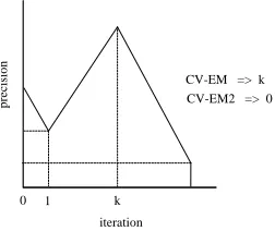
The figure 2 shows a typical case that the CV-EM2 dif-fers from the CV-EM. In the cross validation, the preci-sion is degraded by the first iteration of the EM algorithm, and then it is improved by iteration, and the maximum precision is achieved at thek-th iteration, but the preci-sion converges to the lower point than the precipreci-sion of the iteration number 1. In this case, the CV-EM giveskas the estimation, but the CV-EM2 gives 0.
0 1 k
iteration
preci
sion CV-EM => k
[image:3.612.365.491.573.679.2]CV-EM2 => 0
5
Experiments
To confirm the effectiveness of our methods, we tested with 50 nouns of the Japanese Dictionary Task in SEN-SEVAL2(Kurohashi and Shirai, 2001).
The Japanese Dictionary Task is a standard WSD prob-lem. As the evaluation words, 50 noun words and 50 verb words are provided. These words are selected so as to balance the difficulty of WSD. The number of labeled in-stances for nouns is 177.4 on average, and for verbs is 172.7 on average. The number of test instances for each evaluation word is 100, so the number of test instances of noun and verb evaluation words is 5,000 respectively. However, unlabeled data are not provided. Note that we cannot use simple raw texts including the target word, be-cause we must use the same dictionary and part of speech set as labeled data. Therefore, we use Mainichi newspa-per articles for 1995 with word segmentations provided by RWC. This data is the origin of labeled data. As a re-sult, we gathered 7585.5 and 6571.9 unlabeled instances for per noun and per verb evaluation word on average, respectively.
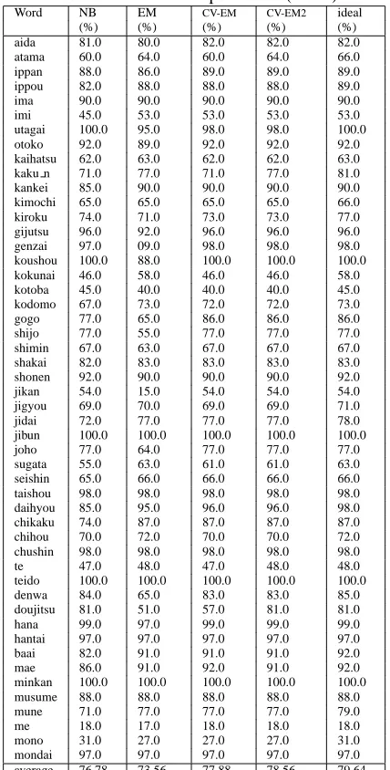
Table 1 shows the results of experiments for noun eval-uation words. In this table, NB means Naive Bayes,
EM the EM method, and ideal the EM method stopping at the ideal iteration number. Note that the pre-cision is computed by mixed-gained scoring(Kurohashi and Shirai, 2001) which gives partial points in some cases.
The precision of Naive Bayes which learns through only labeled data was 76.58%. The EM method failed to boost it, and degraded it to 73.56%. On the other hand, by using CV-EM the precision was boosted to 77.88%. Fur-thermore, CV-EM2 boosted it to 78.56%. This score is a match for the best public score of this task. As success-ful results in this task, two researches are reported. One used Naive Bayes with various attributes, and achieved 78.22% precision(Murata et al., 2001). Another used Adaboost of decision trees, and achieved 78.47% preci-sion(Nakano and Hirai, 2002). Our score is higher than these scores5. Furthermore, their methods used syntactic analysis, but our methods do not need it.
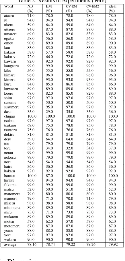
In the same way, we performed experiments for verb evaluation words. Table 2 shows the results. In the ex-periment, Naive Bayes achieved 78.16% precision. The EM method boosted it to 78.74%. Furthermore, CV-EM and CV-EM2 boosted it to 79.22% and 79.26% respec-tively. CV-EM2 is marginally higher than CV-EM.
5
[image:4.612.320.534.99.521.2]The best score for the total of noun words and verb words is reported to be 79.33% in (Murata et al., 2001).
Table 1: Results of experiments (Noun)
Word NB EM CV-EM CV-EM2 ideal
(%) (%) (%) (%) (%)
aida 81.0 80.0 82.0 82.0 82.0
atama 60.0 64.0 60.0 64.0 66.0
ippan 88.0 86.0 89.0 89.0 89.0
ippou 82.0 88.0 88.0 88.0 89.0
ima 90.0 90.0 90.0 90.0 90.0
imi 45.0 53.0 53.0 53.0 53.0
utagai 100.0 95.0 98.0 98.0 100.0
otoko 92.0 89.0 92.0 92.0 92.0
kaihatsu 62.0 63.0 62.0 62.0 63.0
kaku n 71.0 77.0 71.0 77.0 81.0
kankei 85.0 90.0 90.0 90.0 90.0
kimochi 65.0 65.0 65.0 65.0 66.0
kiroku 74.0 71.0 73.0 73.0 77.0
gijutsu 96.0 92.0 96.0 96.0 96.0
genzai 97.0 09.0 98.0 98.0 98.0
koushou 100.0 88.0 100.0 100.0 100.0
kokunai 46.0 58.0 46.0 46.0 58.0
kotoba 45.0 40.0 40.0 40.0 45.0
kodomo 67.0 73.0 72.0 72.0 73.0
gogo 77.0 65.0 86.0 86.0 86.0
shijo 77.0 55.0 77.0 77.0 77.0
shimin 67.0 63.0 67.0 67.0 67.0
shakai 82.0 83.0 83.0 83.0 83.0
shonen 92.0 90.0 90.0 90.0 92.0
jikan 54.0 15.0 54.0 54.0 54.0
jigyou 69.0 70.0 69.0 69.0 71.0
jidai 72.0 77.0 77.0 77.0 78.0
jibun 100.0 100.0 100.0 100.0 100.0
joho 77.0 64.0 77.0 77.0 77.0
sugata 55.0 63.0 61.0 61.0 63.0
seishin 65.0 66.0 66.0 66.0 66.0
taishou 98.0 98.0 98.0 98.0 98.0
daihyou 85.0 95.0 96.0 96.0 98.0
chikaku 74.0 87.0 87.0 87.0 87.0
chihou 70.0 72.0 70.0 70.0 72.0
chushin 98.0 98.0 98.0 98.0 98.0
te 47.0 48.0 47.0 48.0 48.0
teido 100.0 100.0 100.0 100.0 100.0
denwa 84.0 65.0 83.0 83.0 85.0
doujitsu 81.0 51.0 57.0 81.0 81.0
hana 99.0 97.0 99.0 99.0 99.0
hantai 97.0 97.0 97.0 97.0 97.0
baai 82.0 91.0 91.0 91.0 92.0
mae 86.0 91.0 92.0 91.0 92.0
minkan 100.0 100.0 100.0 100.0 100.0
musume 88.0 88.0 88.0 88.0 88.0
mune 71.0 77.0 77.0 77.0 79.0
me 18.0 17.0 18.0 18.0 18.0
mono 31.0 27.0 27.0 27.0 31.0
mondai 97.0 97.0 97.0 97.0 97.0
Table 2: Results of experiments (Verb)
Word NB EM CV-EM CV-EM2 ideal
(%) (%) (%) (%) (%)
ataeru 71.0 78.0 78.0 78.0 78.0
iu 94.0 94.0 94.0 94.0 94.0
ukeru 59.0 64.0 59.0 64.0 64.0
uttaeru 84.0 87.0 87.0 87.0 88.0
umareru 69.0 83.0 82.0 83.0 83.0
egaku 58.0 56.0 56.0 56.0 58.0
omou 90.0 89.0 89.0 89.0 90.0
kau 83.0 83.0 83.0 83.0 83.0
kakaru 58.0 57.0 58.0 58.0 58.0
kaku v 72.0 66.0 72.0 72.0 72.0
kawaru 92.0 92.0 92.0 92.0 92.0
kangaeru 99.0 99.0 99.0 99.0 99.0
kiku 56.0 55.0 55.0 55.0 56.0
kimaru 96.0 96.0 96.0 96.0 96.0
kimeru 93.0 93.0 93.0 93.0 93.0
kuru 84.0 85.0 86.0 85.0 86.0
kuwaeru 89.0 89.0 89.0 89.0 89.0
koeru 78.0 82.0 85.0 82.0 88.0
shiru 97.0 97.0 97.0 97.0 97.0
susumu 49.0 50.0 50.0 50.0 50.0
susumeru 97.0 95.0 97.0 97.0 97.0
dasu 35.0 29.0 35.0 35.0 36.0
chigau 100.0 100.0 100.0 100.0 100.0
tsukau 97.0 97.0 97.0 97.0 97.0
tsukuru 69.0 75.0 78.0 75.0 78.0
tsutaeru 75.0 76.0 76.0 76.0 76.0
dekiru 81.0 81.0 81.0 81.0 81.0
deru 59.0 64.0 64.0 64.0 64.0
tou 69.0 79.0 79.0 79.0 79.0
toru 32.0 34.0 32.0 34.0 37.0
nerau 99.0 99.0 99.0 99.0 99.0
nokosu 79.0 79.0 79.0 79.0 79.0
noru 54.0 54.0 54.0 54.0 54.0
hairu 36.0 36.0 36.0 36.0 36.0
hakaru 92.0 92.0 92.0 92.0 92.0
hanasu 100.0 87.0 100.0 100.0 100.0
hiraku 86.0 94.0 94.0 94.0 94.0
fukumu 99.0 99.0 99.0 99.0 99.0
matsu 52.0 50.0 51.0 51.0 52.0
matomeru 79.0 80.0 80.0 80.0 80.0
mamoru 79.0 71.0 70.0 71.0 79.0
miseru 98.0 98.0 98.0 98.0 98.0
mitomeru 89.0 89.0 89.0 89.0 89.0
miru 73.0 71.0 73.0 73.0 73.0
mukaeru 89.0 89.0 89.0 89.0 89.0
motsu 57.0 62.0 57.0 57.0 62.0
motomeru 87.0 87.0 87.0 87.0 87.0
yomu 88.0 88.0 88.0 88.0 88.0
yoru 97.0 97.0 97.0 97.0 97.0
wakaru 90.0 90.0 90.0 90.0 90.0
average 78.16 78.74 79.22 79.26 79.92
6
Discussion
6.1 Cause of failure of the EM method
Why does the EM method often fail to boost the perfor-mance? One reason may be the difference among class distributions of labeled dataL, unlabeled dataU and test dataT. PracticallyL,UandTare the same because they consist of random samples from all data. However, there are differences among them.
Intuitively, learning by combining labeled data and un-labeled data is regarded as learning from the distribution ofL+U. It is expected that the EM method is effective ifd=d(L, T)−d(L+U, T)>0, and is counterproduc-tive ifd <0, in whichd(·,·)means the distance of two distributions.
To confirm the above expectation, we conduct an ex-periment by using Kullback-Leibler divergence asd(·,·). The distribution ofL+U can be obtained from Equation 4 when the EM algorithm converges. The result of the experiment is shown in Table 3.
Table 3: Effects of the distribution of meanings
d >0 d <0
improvement 6 7
deterioration 2 8
The columns of the table are divided into positive (d >0) and negative (d <0). Positive means thatL+U
gets close toT and negative means thatL+U goes away fromT. The rows of the table are divided into improve-ment of precision and deterioration of precision. In this paper, improvement of precision is when the precision is improved by over 5%, and deterioration of precision is when the precision is degraded by over 5%.
This result indicates that there is a weak correlation be-tween whetherL+U gets close toTor goes away from
Tand whether the EM method is effective or not, but we cannot conclude they are completely dependent. How-ever, the evaluation word ‘genzai’ whose precision falls most by the EM method is precisely the above case. The
dfor this word is the smallest, –0.30, among all evalua-tion words. Further investigaevalua-tion of the causes of failure of the EM method is our future work.
6.2 Effectiveness of estimation of CV-EM2
CV-EM2 achieved ideal estimation for 29 of 50 evalua-tion words, that is 58%. Furthermore, for 15 of the other 21 evaluation words, the difference between the preci-sion through our method and that through ideal estima-tion did not exceed 2%. Therefore, estimaestima-tion of CV-EM2 is mostly effective.
The words ‘kokunai’ and ‘kotoba’ are typical cases where estimation fails. The difference between the pre-cision of CV-EM2 and that through ideal estimation ex-ceeded 5%. The failure of estimation for these two words reduced the whole precision.
Figure 3 compares the precision for cross validation and that for actual evaluation for the word ‘kokunai’. In the same way, Figure 3 shows the case of the word ‘ko-toba’. In these figures, the x-axis shows the iteration number of the EM algorithm. To clarify the change of precision, the initial precision is set to 0, and the y-axis shows the difference (%) between the actual and initial precision.
use-less, so it is difficult to estimate an optimum iteration number in the EM algorithm. However, such cases are rare. In the experiment, this case arises for only this word ‘kokunai’. Consider next the case of ‘kotoba’. In cross validation, the precision improved in the first iteration of the EM algorithm, but got worse step by step thereafter. On the other hand, in the actual evaluation, the precision got worse even in the first iteration of the EM algorithm. The difference of these results in the first iteration of the EM algorithm causes our estimation to fail. In future, we must improve our method by further investigation of these words.
-5 0 5 10
0 2 4 6 8 10
difference from base precision (%)
iteration
[image:6.612.95.273.235.357.2]REAL CROSS-VAL
Figure 3: Comparison between cross validation and ac-tual evaluation (‘kokunai’)
-6 -5 -4 -3 -2 -1 0 1
0 2 4 6 8 10
difference from base precision (%)
iteration
[image:6.612.338.513.247.369.2]REAL CROSS-VAL
Figure 4: Comparison between cross validation and ac-tual evaluation (‘kotoba’)
6.3 Comparison of CV-EM and CV-EM2
CV-EM2 is slightly superior to CV-EM. In the evaluation word ‘doujitu’, there is a remarkable difference between the two methods.
Figure 5 shows the change of the precision for ‘dou-jitsu’ in cross validation, and Figure 6 shows that in ac-tual evaluation.
The precision goes up in cross validation, but goes down largely in actual evaluation. In CV-EM, the best
point is selected in cross validation, that is 3. On the other hand, CV-EM2 estimates 0 by using the relation of three precisions: the initial precision, the precision for the iter-ation 1 and the precision at convergence.
Let’s count the number of words for which CV-EM2 is better or worse than CV-EM. For one word ‘mae’ in nouns and three words ‘kuru’, ‘koeru’ and ‘tukuru’ in verbs, CV-EM was superior to CV-EM2. On the other hand, for four words ‘atama’, ‘kaku n’, ‘te’ and ‘dou-jitsu’ in nouns and four words ‘ukeru’, ‘umareru’, ‘toru’ and ‘mamortu’ in verbs, CV-EM2 was better to CV-EM. These numbers show that our method is somewhat supe-rior to CV-EM.
-6 -5 -4 -3 -2 -1 0 1 2
0 2 4 6 8 10
difference from base precision (%)
iteration
CROSS-VAL
Figure 5: Cross validation in ‘doujitsu’
-30 -25 -20 -15 -10 -5 0
0 2 4 6 8 10
difference from base precision (%)
iteration
[image:6.612.336.512.430.558.2]CROSS-VAL
Figure 6: Actual evaluation in ‘doujitsu’
6.4 Unsupervised learning for verb WSD
[image:6.612.96.271.431.555.2]by the EM method, that is 1.022 times. This shows that the EM method does not work so well for verb words.
We consider that feature independence plays a key role in unsupervised learning. Suppose the instance x con-sists of two features f1 andf2. When class cx of xis judged from featuref1, the probabilityP(cx|f2)is tuned to be larger. The question is whether it is actually right or not to increase P(cx|f2). If it is right, unsupervised learning works well, but if it is not, unsupervised learn-ing fails. Intuitively, feature independence warrants in-creasingP(cx|f2). In noun WSD, the left context of the target word corresponds to the words modifying the tar-get word, and the right context of the tartar-get word cor-responds to the verb word whose case slot can have the target word. Both the left context and right context can judge the meaning of the target word by itself, and are in-dependent. Left context and right context act as indepen-dent features. On the other hand, we cannot find such an opportune interpretation for the features of verbs (Shin-nou, 2002). Therefore, the EM method is not so effective for verb words.
Naive Bayes assumes the independence of features, too. However, this assumption is not so rigid in practice. We believe that the improvement by the EM method for verb words depends on the robustness of Naive Bayes. In our experiments, the EM method for noun words failed to boost the precision. We think that the cause is the im-balance of labeled data, unlabeled data and test data. We should investigate this in a future study.
6.5 Related works
Co-training(Blum and Mitchell, 1998) is a powerful un-supervised learning method. In Co-training, if we can find two independent feature sets for the target problem, any supervised learning method can be used. Further-more, it is reported that Co-training is superior to the EM method if complete independent feature sets can be used(Nigam and Ghani, 2000). However, Co-training requires consistency besides independence for two fea-ture sets. This condition makes it difficult to apply Co-training to multiclass classification problems. On the other hand, the EM method requires Naive Bayes to be used as the supervised learning method, but can be ap-plied to multiclass classification problems without any modification. Therefore, the EM method is more prac-tical than Co-training.
Yarowsky proposed the unsupervised learning method for WSD(Yarowsky, 1995). His method is reported to be a special case of Co-training(Blum and Mitchell, 1998). As two independent feature sets, one is the context sur-rounding the target word and the other is the heuristic of ‘one sense per discourse’. However, it is unknown how valid this heuristic is for granularity of meanings of our evaluation words. Furthermore, this method needs
doc-uments in which the target word appears multiple times, as unlabeled data. Therefore, it is not so easy to gather unlabeled data. On the other hand, the EM method does not have such problem because it uses sentences includ-ing the target word as unlabeled data.
6.6 Future works
We have three future works. First, we must raise the pre-cision for verb words, which may be impossible unless we use other features, so we need to investigate other fea-tures. Second, we must improve the estimation method of the optimum iteration number in the EM algorithm. The difference between the precision through our estimation and that through the ideal estimation is large. We can im-prove the accuracy by improving the estimation method. Finally, we will investigate the reason for the failure of the EM method, which may be the key to unsupervised learning.
7
Conclusions
In this paper, we improved the EM method proposed by Nigam et al. for text classification problems in order to apply it to WSD problems. To avoid some failures in the original EM method, we proposed two methods to esti-mate the optimum iteration number in the EM algorithm. In experiments, we tested with 50 noun WSD problems in the Japanese Dictionary Task in SENSEVAL2. Our two methods greatly improved the original EM method. Es-pecially, the score of noun evaluation words was equiva-lent to the best public score of this task. Furthermore, our methods were also effective for verb WSD problems. In future, we will tackle three works: (1) To find other effec-tive features for unsupervised learning of verb WSD, (2) To improve the estimation method of the optimum itera-tion number in the EM algorithm, and (3) To investigate the reason for the failure of the EM method.
References
Avrim Blum and Tom Mitchell. 1998. Combining La-beled and UnlaLa-beled Data with Co-Training. In 11th Annual Conference on Computational Learning The-ory (COLT-98), pages 92–100.
Sadao Kurohashi and Kiyoaki Shirai. 2001. SENSEVAL-2 Japanese Tasks (in Japansese). In Technical Report of IEICE, NLC-36–48, pages 1–8.
Cong Li and Hang Li. 2002. Word Translation Dis-ambiguation Using Bilingual Bootstrapping. In 40th Annual Meeting of the Association for Computational Linguistics (ACL-02), pages 343–351.
Masaki Murata, Masao Utiyama, Kiyotaka Uchimoto, Qing Ma, and Hitoshi Isahara. 2001. CRL at Japanese dictionary-based task of SENSEVAL-2 (in Japanese). In Technical Report of IEICE, NLC-36–48, pages 31– 38.
Keigo Nakano and Yuuzou Hirai. 2002. AdaBoost wo motiita gogi no aimaisei kaisyou (in Japanese). In 8th Annual Meeting of the Association for Natural Lan-guage Processing, pages 659–662.
Kamal Nigam and Rayid Ghani. 2000. Analyzing the effectiveness and applicability of co-training. In 9th International Conference on Information and Knowl-edge Management, pages 86–93.
Kamal Nigam, Andrew McCallum, Sebastian Thrun, and Tom Mitchell. 2000. Text Classification from Labeled and Unlabeled Documents using EM. Machine Learn-ing, 39(2/3):103–134.
Seong-Bae Park, Byoung-Tak Zhang, and Yung Taek Kim. 2000. Word sense disambiguation by learning from unlabeled data. In 38th Annual Meeting of the Association for Computational Linguistics (ACL-00), pages 547–554.
Hiroyuki Shinnou. 2002. Learning of word sense disambiguation rules by Co-training, checking co-occurrence of features. In 3rd international conference on Language resources and evaluation (LREC-2002), pages 1380–1384.