Abstract—In this paper a theoretical study of a new Spray On Demand print-head (SOD) is performed. This work leads us to study (i) fluid structure/interaction with a vibrating tube conveying fluid, assimilated to a cantilever beam excited by a pointwise piezoactuator (PZA) (ii) fluid film instability with spray generation. After establishing a more general equation of the motion of a vibrating tube filled with fluid using Hamilton’s modified principle, an analytical solution is proposed allowing to determine the volume flow rate generated by the motion of the tube motion. The maximum entropy formalism (MEF) is used to predict the drop size distribution and the Sauter Mean Diameter of the SOD. The coupling of the three-parameter generalized Gamma distribution with physical based-distribution constraints is proposed leading to new predictions in the framework of the MEF formalism.
Index Terms— Tube conveying fluid, Vibration, Hamilton’s modified principle, Spray, Maximum Entropy Formalism.
I. INTRODUCTION
A great number of engineering applications are concerned with the dispense of minute quantities of fluid [1], [2]. Whereas it is familiar to use ink-jet print-heads for printing with ink in the graphics industry; this technology offers an amazingly broad range of adaptability in wide range areas as in biomedicine, electronics, pharmacology, micro-optics, and many others limited only by our imagination. However these different applications need printing devices more or less robust. Printing technique could be classified in three categories with respect to their performance: Drop On Demand (DOD), Continuous Ink Jet (CIJ), electro-valve and spray technologies. DOD classes are well known technologies for graphic art industries and now more and more used for micro-deposition. While CIJ is much more dedicated for coding and marking applications even if more recently it is also used for commercial very high speed printings. This technology could also be able to jet
Manuscript received March 21, 2008.
M. Tembely is with the LEGI-Laboratory of Geophysical and Industrial Fluid Flows-, UMR 5519, University Joseph Fourier, Grenoble, BP 53,
38041 Grenoble cedex, France.(corresponding author phone:
(00)33-456-521-120, fax:(00)33-475-561-620, e-mail: [email protected]).
Prof. C. Lecot is with the LAMA-Laboratory of Applied Mathematics-, UMR 5127 CNRS, University of Savoie, 73376 Le Bourget-du-Lac Cedex, France
(e-mail: [email protected]).
Prof. A. Soucemarianadin is with the LEGI-Laboratory of Geophysical and Industrial Fluid Flows-, UMR 5519, University Joseph Fourier, Grenoble, BP 53, 38041 Grenoble cedex, France
(e-mail: [email protected]).
micro-deposit quantities for deep penetration on porous substrate.
For high throughput device, electro-valve technologies is used mainly for coding and marking secondary packaging like box, we can find those technologies also to print long mesh fabrics such as carpets, but those technologies are dedicated for large volume of liquid jetting. Finally, Spray Technology, largely used for paint sprays guns (mix of air and liquid or air and toner), though our work will focus on a new finer spray technology, which could be qualified as a Spray On Demand (SOD) print-head technology. Generally classical print-heads are adapted to applications dealing with Newtonian fluids. However large engineering applications need robust devices allowing ejection of rheological complex fluid (like polymer). Here we present and undertake a theoretical study of the new Spray On Demand device (SOD). The applications covered by this device range from ejection of complex fluid (polymer), fuel cell fabrication, jet printing metallization (copper and gold electrodes) by electroless plating based in our pending patent on impervious and porous substrate.
From a theoretical point of view the study of the new spray on demand device, leads us to study one of the most intriguing problems (i) fluid structure/interaction with vibrating tube conveying fluid, assimilated to a cantilever beam. It is to be noticed here that many engineering application deals with fluid flow fluid in cantilever tube. These applications range from nuclear power plants, fuel carrying tube, medicals devices and many others applications [12], [13], [28]. These problems have been studied theoretically and experimentally for nearly half a century. The complexity of the interaction fluid/structure associated with boundary moving condition, as in our case, is one of the most interesting and difficult problem in dynamical system; (ii) fluid film instability with spray generation. Due to the wide range applications of the new SOD, interest in the size and velocity distribution of droplets is obvious, since in some applications droplet size distribution must have a particular form. There is profuse literature discussing the prediction of representative drop diameter in spray. However, there are relatively few publications dealing with drop size distribution prediction. One of the mean to describe quantitatively a spray is thus to adopt the tools of statistical analysis. Following [31], there are three methods for modeling drop size distribution: discrete probability function, empirical method and Maximum Entropy Formalism (MEF) [21]. The latter is the one adopted to predict the drop size distribution of the SOD.
The modeling of this problem is more complicated than those implied tube vibration in the literature due to the external pointwise force of the piezo-actuator (PZA) and fluid film instability leading to spray generation.
Obviously our findings will be easily extendible to the many others applications implied such a consideration.
Moussa Tembely, Christian Lecot and Arthur Soucemarianadin
A.Presentation of the new spray on demand device
The new Spray On Demand device (SOD) mark traded as Flatjet® is a new liquid dispensing device [3], [4] with high throughput printings, simple and of robust construction.
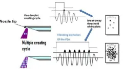
In this technology the coupled fluid/structure vibrations of a nozzle make possible to obtain pulverization with a given angle. The process aims at various applications of new technologies ranging from ejection of pico-to-micro-liter, Newtonian, to non-Newtonian fluids. This technological process makes possible to diffuse by spraying complex fluids through a tube vibrating by a piezoceramic component placed in its middle (Fig. 1).
In the next sub-sections we propose the principle, modeling and prediction of the drop-size generated by the print-head.
Flexibilities and precisions offered by Flatjet® make it ideal candidate for different manufacturing applications to which we will be back later. That is the reason among others our study be focused on the theoretical understanding of the device so that to improve it.
B. Principle of SOD operating: from nozzle vibration to atomization
The principle of spray formation is due to Faraday instability provoked by ultrasonic vibration of the tube [5]. It is a parametric resonance in which instability modes on hung drop at the SOD needle tip appear when a critical acceleration value is reached. As proposed by many authors [6]-[8] when exciting frequency is a multiple of vibrating frequency of the free surface, the first instable mode is a sub-harmonic frequency equal half of the exciting frequency. The limit acceleration in which droplet is generated depends on the exciting frequency, fluid and tube (structure) properties. The acceleration exerted on the fluid at the nozzle tip (Fig. 2) could be expressed as:
A
a
∝
ω
2 (1) where we assume a sinusoidal displacement of the SOD beveled tip. Respectively a, ω, A are acceleration, pulsation and amplitude of the film at nozzle tip.So when the limit acceleration at which film instability occur is known we easily can deduce the maximum amplitude of the film at which instability generates droplets leading to atomization:
2
/
ω
la
A
∝
(2) This amplitude is about some micrometers for classical ultrasonic spray generator [8]. [image:2.595.362.482.50.118.2]The existence of this limit acceleration allowing droplet generation is the principle exploited by the SOD device. In fact as sketched in Fig.2, when the tip acceleration reach the limit acceleration al atomization takes place. The number time per cycle in which this limit is reached give the density of droplets generated by the SOD.
[image:2.595.323.527.657.738.2]Figure 1: Principle of Flatjet® print-head and visualization of the spray
Figure 2: principle of spray generation
Then to complete modeling of the SOD, we need to know displacement and/or acceleration at the tip of the nozzle coupling with the fluid motion inside the tube.
Before carrying out further analysis, we need to determine the force exerted on the nozzle by the piezo-ceramics actuator (PZA) as show in Fig. 1.
C. Piezoelectric Actuator (PZA) modeling: force determination
The SOD nozzle vibrates due to the soldered piezoceramic disc movement. Here we propose to determine the force exerted by the PZA on the needle knowing the voltage wave form applied to the actuator.
We model the relationship between the voltage Vp applied to the PZA to the radial force generated by:
31
2 g
V r
Fp p p
π
= (3) Where Fp is the radial force, rp is PZA radius. Whereas g31 is piezoelectric voltage constant (Vm/N). For further information on piezo-ceramic applications and uses see [9], [10].
We extend (3) for a sinusoidal excitation of the PZA, with the voltage of the following form
) 2 sin( )
(t A ft
Vp = p πr with Ap=5V,fr=150kHz,rp=2cm, )
/ ( 310 .
7 3
31 Vm N
g =− − .
This force and of sine form is not a restriction as any other force could be broken down through Fourier decomposition series. In addition, linking the force with the characteristics of PZA is a very useful approach for a comprehensive modeling of SOD. So that parametric study and effect of PZA properties on SOD operation be possible.
II. FLUID/ TUBE EQUATION OF MOTION
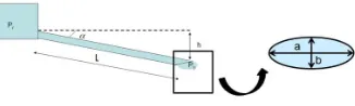
We consider the system as an approximation of the SOD shown in Fig. 3. A straight cantilever tube is fixed along the x-axis. The fluid enters the tube at the fixed end and exits at the free end. At the middle of the tube is soldered a piezoelectric actuator allowing transversal motion of the nozzle. The free end of the tube is beveled.
[image:2.595.95.244.678.725.2]The exerted force generated by the piezoelectric actuator induces a vibrating motion of the tube. Unlike the unconstrained pipe dynamical stability done by many others [11]-[13], our system aim is quite different in the way that we want to cause the meniscus droplet at the nozzle tip to break-up, leading to spray generation.
We decompose the problem in order to evaluate the fluid-flow and PZA fixation effect on tube vibrating motion. For this purpose, the first consideration will be only “structural” without fluid, the second be the coupling between fluid and structure interaction. Analytical solutions are proposed for these two cases with an external punctual excitation force. We conclude by applying these results to predict the flow rate generated by tube motion and of the drop size distribution by new formulation of the Maximum Entropy Formalism. An analytical expression will be proposed for as well as Sauter Mean Diameter(SMD) and drop size distribution of the SOD. Firstly, we start by establishing a more general formulation taking into account PZA position effect, non-linear and other configurations of the SOD depicted in Fig. 5.
Hypothesis
Let establish the equation motion of the annular tube with an external force on the tube with the following hypothesizes. Standard hypothesis for these development assumes,(i) the tube is of uniform annular cross-section, (ii) tube is long compared to its diameter (iii)effect of rotary inertia and shear deformation are ignored, (iv) center line of the tube is inextensible(v) tube is elastic and initially straight, (vi)plane sections remain plane and perpendicular to the beam axis (Bernoulli-Euler beam theory) (vii) effect of internal dissipation and damping are neglected.
A.General fluid/tube equation of motion with PZA position effect
It is to be stressed here that our analysis is not for high speed flow where flutter instability (via a Hopf bifurcation) is observed once the flow velocity exceeds a critical velocity [12]-[14]. The dynamical stability analysis and flutter instability control of pipes conveying fluid has been done by many authors [11], [15], [28]. For our case, let us establish the equation of motion for fluid flowing inside the tube using the elegant Hamilton Principle taking into account non-linear and SOD configuration effect.
At rest the tube extends along the x-axis of a Cartesian co-ordinate system (Fig. 3). Since the tube is inextensible the arc-length along the deformed tube coincides with the x in the underformed state and it can be used as a material variable. Following [19], let the location of a material point on the tube be given by
j y i x j t s v i t s u s r
r r r r
r
+ = +
+
=( ( , )) ( , ) (4) Where i
r
, j
r
, k
r
are fixed orthogonal unit vectors. And x, y, are Euleurian coordinate.
Since the tube is inextensible and along the x-axis, the curvilinear coordinate is as s>>u(s,t) , axial elongation is negligible.
The unit tangent tr vector is then
s r t
∂ ∂ =
r
r (5)
And the normal vector,
n
r
, is given byn
s tr r
κ
= ∂
∂ (6) nr,tr, are thus determined by
v
the transversal displacementof the tube, κ denotes for the curvature.
During the tube motion the loading is due to the acceleration of the tube and the fluid as well as the punctual force. Let
m
and M be the mass per unit length of the tube and fluid, respectively. Then we deduce:
2 2
) , (
t t s r m
∂
∂ r as the inertial force per unit length of the tube And
2
2 (,)
dt t s r d M
r
as the inertial force per unit length due to fluid. Where material derivative with respect to the fluid is given
s U t dt d
∂ • ∂ + ∂
• ∂ = •
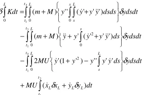
As previously mentioned this study will be carried out by using the modified Hamilton’s principle. The aim is to establish the more general equation of motion of the tube by taking into account different effect. Hamilton formulation seems to be the most convenient for our study, it could be formulated as follows [11], [16], [18] :
∫
∫
∫
+ =2
1 2
1 2
1
t
t t
t
L L t
t
dt r dt
r d MU Wdt
dt r
r
l δ δ
δ (7)
The determination of the different terms of this equation will lead to a more general equation of motion of the nozzle conveying fluid. Here we will take into account non-linear terms, gravity effect and PZA position. In (1)
l
represents the Lagrangian of the system given by,t t f
f V K V
K − + −
=
l (8)
l
is composed of fluid and tube Lagrangian, respectively in turn represented by the sum of kinetic K and potential energy V , subscripts f and t denote for fluid and tube.W
δ represents the virtual work accounting for forces not included in the Lagrangian.
M
F W
W
W δ δ
δ = + (9)
F
W
δ represents the virtual work to due to PZA excitation force. And δWM virtual work due to moment created by PZA fixed on the tube, this effect takes into account the fact that the PZA is not soldered to the center line of the tube as classical analysis could assume, instead of the boundary of the tube. Then, soldered position of PZA engenders moment during SOD operating. In (7) the right-hand term represents the momentum transport due to fluid motion across the open surface of the tube.
In the following sub-sections, we will determine the expression of the different terms of (7) mentioned above. Before we recall some useful relationship, for the curvature
2 2 2 2 2 2
2 ( ) ( )
s v s
u ∂ ∂ + ∂ ∂ =
κ (10) and the inextensible condition
1 ) ( ) ( ) ( ) 1
( 2 2 2 2
2
= ∂ ∂ + ∂ ∂ = ∂ ∂ + ∂ ∂ + =
s y s x s v s u t
r (11)
Kinetic energy of the system
The kinetic energy of the system consists of the kinetic energy of the fluid and of the tube:
∫
∫
+= + =
L t L
t
f ds m v ds
dt r d M K K K
0 2
0 2
2 1 ) ( 2
1 r (12) Where fluid and tube velocity are given by
r s U t dt
r
dr r
) (
∂ ∂ + ∂
∂
= and
t r vt
∂ ∂ =
r
dt y y x x MU ydsdt ds y y y y y MU ydsdt ds y y y y y M m ydsdt dsds y y y y M m Kdt L t t L L L t t L L s t t L s t t
L s L
s L ) ( ' ' '' ) ' 1 ( ' 2 ) ' ' ' ( ' ) ( ) ' ' ' ( '' ) ( 2 1 2 1 2 1 2 1 0 2 0 0 2 0 0 0 δ δ δ δ δ δ
∫
∫∫
∫
∫∫
∫
∫∫
∫∫
∫
+ + − + − + + + − + + = & & & & & & & & & & & & (13)Here prime (’) and (.) respectively denotes for derivative with respect to s (or x) and t.
Potential energy of the system
There are 2 components for the potential energy of the system. The strain energy of the tube Vt and gravitational energy Vg for both fluid and tube structure.
g
t V
V
V= + (14)
The potential energy due to gravity for both fluid and structure is − + = + − = − =
∫
∫
∫
∫
L L L Lg Frds m M grds m M g yds xds
V 0 0 0 0 sin cos ) ( . ) (
.r rr α α
r (15)
Finally, we obtain, using (11):
∫ ∫ ∫ ∫ ∫ ∫ ∫ + + + − + − + + = 2 1 2 1 2 1 2 1 0 0 2 0 3 cos ) ( ) '' ' 2 3 " )( ( sin ) ( ) ' 2 1 ' ( sin ) ( t t L t t L t t L t t g ydsdt g M m ydsdt y y y s L g M m ydsdt y y g M m dt V δ α δ α δ α
δ (16)
About the strain energy of the tube we have:
∫∫
∫
= 2 1 2 1 0 2 ) ( 2 1 t t L t ttdt EI dsdt
V δ κ
δ (17)
Where 2
κ the curvature squared given by (10). After some algebraic manipulations, we find
∫ ∫
∫
= + + + 2 1 2 1 0 2 3 ) " " ' ' " " ' 4 " '' '' ( t t L t ttdt EI y y y y y y y ydsdt
V δ
δ (18)
Virtual work
To establish the virtual work due to piezo-electric displacement along the y-axis.
∫ ∫
∫
∫
= =− − 2 1 2 1 2 1 0 ) ( ) ( ) , ( t t L P s t t t tFdt F xt j rdt F t x x ydsdt
W δ δ δ
δ r r (19)
Here we have admitted as previously mentioned a punctual force j x x t F j t x
F s P
r r ) ( ) ( ) ,
( = δ − (20) Do not confuse Hamilton operator to the Dirac delta function. The effect of the PZA fixed point could be estimated by the following moment calculus
k t x F t x F M r r r r θ ς ς× ( , )= ( , ) sin
= (21)
' tan
sinθ≈ θ=y (22) θ
δ
δWM =Mr r (23)
Where θ is the local angle of deflection of the tube and
ς
its inner radius. We finally obtain:∫ ∫
∫
= − 2 1 2 1 0 '' ) ( ) ( t t L P s t tMdt F t x x y ydsdt
W ςδ δ
δ (24)
The right-hand side of equation (7) could be express as:
∫∫ ∫ ∫ ∫ − + + + = 2 1 2 1 2 1 0 2 2 "(1 ') " ' "
) ( t t L L s L t t L L L t t L L ydsdt ds y y y y y MU dt y y x x MU dt r dt r d
MU δr &δ &δ δ
r (25)
Replacing the different terms (13), (16), (18), (19), (24), (25), in (7) leads us to the general equations motion of the problem where for convenience we have replaced the transversal displacement previously denoted
y
byv
in agreement with (4).{
}
0 " ' " ) ' 1 ( " ' ' ' ' ) ' 1 ( ' 2 cos ) ' ' ' 2 3 " )( ( sin ) ' 2 1 ' ( sin ) ( ) ' ' ' ( ' ) ' ' ' ( ' ' ) ( ) 1 ' ' )( ( ) ( ) ' " " ' 4 " ( ' ' ' ' ) ' 1 ( 2 2 2 2 3 0 0 2 3 2 = − + + − + − + + − − + + + + + − + + + − − + + + + ∫ ∫ ∫ ∫ ∫ L s L s s L s s P s ds v v v v v MU ds v v v v v MU v v v s L v v g M m ds v v v v v dsds v v v v M m v x x t F v v v v v v EI & & & & & & & & & & α α α ς δ (26)Numerical methods could be used to solve this equation as is done for dynamical analysis, but for our needs to have analytical solution especially for MEF applications to spray; some simplications of (26) during our modeling of the SOD are made.
B.Structural equation of motion: cantilevered beam
approximation
The equations of motion is established here from (26) by neglecting the fluid effect, non-linear, and gravity. Subsequent developments based on Euler beam theory, will allow us to deduce an analytical solution of the (hollow) tube subjected to an external punctual force.
Cantilevered beam
From (26) and after making it dimensionless by L (beam length) and using the same symbol for convenience, we retrieve vibrating equation for the nozzle, assimilated to cantilevered hollow tube:
) , ( ) ( 2 2 2 2 4 2 2 t x f t v S x v L EI
x ∂ =
∂ + ∂ ∂ ∂ ∂
ρ (27)
With x=x/L
[image:4.595.72.214.50.144.2]Where f(x,t)=Fs(t)δ(x−xp)/L is a punctual force per unit length applied at a specific point of the tube.
Table I: Some parameters used for the calculation
L Nozzle lenhght 0.05 (m)
xp dimensionless position of the punctual force 0.5 g gravity acceleration 9.81 m/s2
R outer radius of the tube 0.0005(m)
ς inner radius of the tube 0.00025(m) ( 2 2)
ς
π −
= R
S annular area of the nozzle
) ( 2 4 4 ς π − = R
I quadratic inertia of the tube
EI Flexural rigidity 0.01839843750 (SI)
t
ρ tube density 7800 kg/m3
f
ρ fluid density 1000 kg/m3 m S
t ρ
= Masse per unit length of the tube
M S
f ρ
= Masse per unit length of the fluid
U average velocity in the tube 1 m/s µ fluid viscosity 0.001 Pa.s
σ fluid surface tension 0.07 N/m f vibrating frequency of the PZA 150kHz
Galerkin’s method is used to determine unsteady solution decomposed in orthonormalized mode
) ( ) ( ) , ( 1 x V t q t x v N i i i
∑
=i
V orthonormal mode determined thanks to free vibration equation 0 ) ( 2 2 2 2 4 2 2 = ∂ ∂ + ∂ ∂ ∂ ∂ t v S x v L EI x ρ (29) Classical variables separation method is used with,
) ( ) ( ) ,
(xt V xT t
v = , leading to
0 ) ( 4 2 4 4 = − V EI L S x dx V
d ρω (30) Letting β4 =(ρSω2L4)/EI and boundary condition,
0 '= =V
V and V''(1)=V'''(1)=0, we deduce,
) cosh( ) cos( ) sinh( ) sin( )
(x A x B x C x D x
V = β + β + β + β (31)
Using boundary condition for V(x) in (31), lead to the following classical transcendental equation:
0 1 ) cosh( )
cos(β β + = (32) And iterative method with an initial guess of
2 / ) 1 2 ( ) 0 ( π
βi = i− allow to compute vibrating mode from (32)
In other hand, an asymptotic approximation could be found as follow:
k
k k ε
π α = − +
2 ) 1 2 (
Using in (32) we compute the correction
ε
k, so that to find a good approximation: − − + − = ≈ − 2 ) 1 2 ( cosh / ) 1 ( 2 ) 1 2( π 1 π
α
β i i i
i i
Finally, Vi(x) could be expressed as:
) ( ))] cosh( ) (cos( ) cosh( ) cos( ) sinh( ) sin( ) sinh( ) [sin( )
(x A x x x x A x
V i i i i
i i i i i i i
i β β β β φβ
β β β
β − =
+ + − − = (33) We determine Aiso that to normalize Vi with respect to the following normalization condition.
∫
= 1 0 2 1 dx SVi ρFrom (33) then Ai is given by
∫
= 1 0 2 ) ( 1 dx x S A i i β φ ρ (34)A tiresome calculus leads us to
))) sinh( ) sin( 4 ) 2 (cosh( )) sinh( ) cos( ) sin( ) cosh( ( )) cosh( ) cos( 1 ( 6 ) 2 cos( ( )) cosh( ) (cos( 2 1 ) ( 2 1 0 2 i i i i i i i i i i i i i i i
ixdx
β β β β β β β β β β β β β β β β φ + + + − • + + − + = ∫
Substituting (28) in (27), multiplying by Vj and integrating along the bar from 0 to 1, one find, using modes ortho-normalities properties:
∫
= = + 1 0 2 ) , ( ) ( ) ( )(t w q t Q t Vf xtdx
q&i i i i i
& (35)
The pointwise force per unit length can be modelled by letting ) ( ) ( ) ,
(xt Fp t x xp
f = δ − (36) With δ a one dimensional Dirac function, where xp is the point at which PZA is applied on the nozzle, where Fp(t) is given by (3).
To buckle the loop, it is necessary to solve the ODE (35) on q(t) by using the Laplace transform and its inverse:
By taking1
) sin( )
(t F t
F = p Ωp (37)
1
Note that this not an restriction since any function could be decomposed into Fourier series, in other hand this force seems to approach the most the one exerted by the PZA on the nozzle.
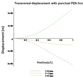
We deduce, 2 2 2 )) sin( ) sin( ( ) ( ) ( p i p i i p i p i p i t t x V F t q Ω − Ω − Ω = ω ω ω ω (38) Finally by taking (33), (34), (37) and (38) we obtain an analytical solution (28) of the beam exited by a pointwise sinusoidal force, the solution converges with just few term on the sum (Fig. 4) at different instant times using Table I. The displacement of the nozzle tip is about some micrometers in agreement with what it is observed experimentally when the SOD operates.
C.Linear fluid/tube equations of motion
Here we establish the equation of motion of the nozzle conveying fluid by neglecting non-linear, gravity and PZA position effect from (26) or see (Appendix), and making the equation motion dimensionless, we obtain:
) , ( 2 2 2 2 2 2 1 4 4 t x f x t v c t v x v c x v = ∂ ∂ ∂ + ∂ ∂ + ∂ ∂ + ∂
∂ (39)
where 2
2
1 U
EI ML
c= , ,
) ( 1 2 2 M m EI LU c +
= 2 ,
EI M m
L +
=
τ (,) (,),
3 t x F EI L t x f =
To solve (39), we seek the solution in the following form:
) , ( ) , ( ) ,
(xt v0 xt v1 xt
v = + (40) where
v
0(
x
,
t
)
is given by (28) andv
1(
x
,
t
)
takes into account the effect of velocity inside the tube.Replacing (40) in (39) and making time again dimensionless by using the resonance frequency (fr ) of the PZA such that
r
f
t
t
=
/
τ
leads us to:x t v f c x v c x t v f c t v f x v c x v r r r ∂ ∂ ∂ − ∂ ∂ − = ∂ ∂ ∂ + ∂ ∂ + ∂ ∂ + ∂
∂ 20
2 2 0 2 1 1 2 2 2 1 2 2 2 1 2 1 4 1 4 )
( τ τ (41)
The right-hand term of (41) is known. For finding analytical solution we will furthermore make assumptions in order to get an approximate solution of (41). According to the problem parameter, we could admit the following estimation
; 1 ,
1 ∝
∝ x
t c1<<1,c2∝1,( ) 1,
2 >>
r
f
τ
with the rigidity of the tube we could assume easily that
)
,
(
)
,
(
01
x
t
v
x
t
v
<<
.Finally the equation to be solved is:
x t v c x v c t v ∂ ∂ ∂ − ∂ ∂ − = ∂ ∂ 0 2 2 2 0 2 1 2 1 2 (42) Where only the second-derivative temporal term dominates on the left-hand term in (39).
[image:5.595.351.497.612.748.2]Then, we can easily deduce the theoretical solution of the problem.
dt d x
t x v c dt d x t
v c x
v c t x
v
∫ ∫
t∫ ∫
t∂ = ∂ + ∂ ∂ ∂ − ∂ ∂ − =
0 0 2
0 2 1 0 0
0 2 2 2
0 2 1
1 )
) , 0 ( ( )
( ) ,
( τ τ τ τ (43)
The second term on the right-hand allow to impose
0 ) , 0 (
1 x= t =
v .
As shown in Fig. 5, the velocity effect on tube motion can be negligible when comparing to the case without fluid (Fig. 4).
III. VIBRATING TUBE FLOW RATE ESTIMATION
We would like here to propose a new approach allowing for determining the flow rate Q due to the vibrating motion of the tube.
The movement of the fluid in the tube is subjected to viscosity effect because of the size of the nozzle where the flow takes place. The question to be answered is how to express the forcing term causing fluid motion in the channel.
Following irreversible thermodynamics [29], [30] expressing the proportionality between flux and force,
kf
Q= (44) f is the force, k coefficient of proportionality
In case of fluid flowing in the channel, the flux could be expressed as [20]:
L P µ
Q /
8
4
∆
=πς (45)
Where
ς
is the inner radius of the tube andµ
is the fluid viscosity, ∆P/L being pressure gradient along the tube. When the force is only due to hydrostatic pressure, it expresses as:g L P
f =∆ / =ρ (46)
An interpretation of (46) stipulates that force is caused by gravity acceleration.
When we neglected the inclination of the tube, we can express the pressure on the tube in following form implying transversal (vertical) displacement of the tube.
) , (xt gv
P=ρ (47) Then, pressure gradient is given by:
) , ( ' xt gv dx dP
ρ
= (48)
In our case, and making an analogy analysis with (46) for the force, the acceleration is not only g but also includes the acceleration of the tube, so incorporated this acceleration in (48) and using a root mean square operator, we express the force causing flux in tube in the following form:
t
t
x
v
t
x
v
g
f
=
ρ
<
(
−
&
&
(
,
))
'
(
,
)
>
(49) Where the root mean square operator is defined as∫
• = > •< 1
0 2
dx
[image:6.595.322.525.558.626.2]t
Figure 5: Effect on displacement of fluid flow motion inside the nozzle.
∫
−= 1
0
2 4
)] , ( ' )) , ( [( 8 )
( g vxt v xt dx
µ t
Q ρπς && (50)
Where v(x,t) is the solution of (39) approximated by (40), in that case v(x,t) is function of mean velocity in the tube U which is defined as Q/As where As is the area of the tube section. So, (50) is an implicit equation for Q(t) = F(Q(t)). However, as shown previously in II.C where we neglect the effect of fluid velocity
v
(
x
,
t
)
≈
v
0(
x
,
t
)
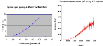
, we can compute relatively easily the flow rate from (50) see (Fig.6 a-b). From (50), we deduce the volume ejected when the SOD operates in following form:τ τ
τQ d
t V
t ol =
∫
0
) ( )
( (51)
As shown in Fig. 7, theoretical results compare qualitatively well with experimental results. In the author knowledge that a first such an approximation is proposed for vibrating tube conveying fluid.
IV. SODSPRAY MODELING:SAUTER MEAN DIAMETER AND
PREDICTION OF DROP-SIZE DISTRIBUTION
The significant number of drops constituted a spray does not allow to precisely determining the diameter or the velocity of each drop. There is profuse literature discussing the prediction of representative drop diameter in spray [23]-[27], [31]. However, there are relatively few publications dealing with drop size distribution prediction. One of the mean to describe quantitatively a spray is thus to adopt the tools of statistical analysis. Following [31], there are three methods for modeling drop size distribution: Empirical Method, Probability Function Method and the Maximum Entropy formalism (MEF) which is the one adopted by us.
A. Applications of MEF to SOD spray generation
[image:6.595.322.526.663.754.2]The constraints contained in the MEF could be chosen as, in the case of our SOD spray, laws of conservation (mass, energy) written before and after the break-up of liquid film at nozzle tip. For spray formation one can consider that at a certain time a volume of liquid ejected by the SOD nozzle
Figure 6: Flow rate Q (m3/s) during SOD operating relatively (a) long time
and (b) short time.
Figure 7: Ejected volume during SOD operation (a) experimental (b)
during a fixed excitation time is completely fragmented in a number N of spray droplets. These droplets diameter follow a certain determined distribution.
We would like to determine the Sauter Mean Diamter and droplet size distribution of the original Spray On Demand print-head, theoretically via the MEF method. For this purpose we need to express the different constraint physically imposed to the spray. We choose to express mass and energy conservation.
Before starting the calculation let’s make some precision on the MEF use in our SOD device. We assume that the drop diameter space is divided into classes noted as
] 2 / , 2 /
[Di−∆Di Di−∆Di , and Ni the number of drops in each
class, it is possible to build the histogram of the frequency of occurrences of a given class. We denote pithe histogram of the number-based probability distribution whereas the continuous version of the histogram is a probability density function, referred as the number-based drop-size distribution with notation fn(D). Similarly, volume-based distributions fv(D) could be defined, and Vi , Si being defined respectively as droplet volume and surface in class i.
Mass conservation
Let Msbe the mass of fluid ejected by the needle during a fixed excitation time T. We can express Msdifferently in the following way:
∑
∑
==
= ol i
s V mi V
M ρ ρ (52)
3 30 3
3
6 6
6 ND N pD D
Vi ρπ i i ρπ i i ρπ
ρ =
∑
=∑
=∑
(53)Where
i
p is defined as pi=Ni/N. From (53) we deduce the constraint upon mass conservation as:
∑
p
id
i3=
1
with30 D
D
d i
i = (54)
Before starting with the second constraint, let’s express Ms
in term of operating conditions and fluid properties.
At the tip of the needle, by apply Newton second law, with a balance between inertial force surface tension and gravity. Considering the droplet size at the needle tip, we cannot neglect the gravity effect, since Bond number based on tube diameter is
2 . 0 ) 2 ( 2
∝ =
σ ς ρg Bo
We propose to express the balance equation in the following form in addition to gravity we introduce nozzle tip acceleration. Because, we can reasonably assume that gravity as well nozzle tip motion contribute to hung drop falling and break-up. So, we deduce
E
s g C
M (γ+ )=σ cosθ (55)
[image:7.595.376.471.53.140.2]Equation (55) is quite different from static analysis of dripping from a vertical tube see [20].
Figure 8: drop hanging on the nozzle tip and nozzle boundary geometry
Figure 9: Nozzle tip acceleration ()( / 2)
s m t
γ compute from previous
model in II.
In (55) θEis the equilibrium contact angle between fluid and nozzle structure, σ fluid surface tension, C being the circumference of the elliptical droplet contact shape.
) (
4aE e
C= (56) The circumference of an ellipse being C=4aE(e) where the function E is the complete elliptic integral of the second kind:
∑
∞∏
= =
−
−
− =
0
2 2
1 2 1
) 2
1 2 ( 2
n
n n
m n
e m m a
C π (57)
A good approximation due to Ramanujan is given by
)] 3 )( 3 ( ) ( 3
[ a b a b a b
C≈
π
+ − + + (58)Where e is eccentricity, a semi-major axis, b semi-minor axis (Fig. 8).
The acceleration of the needle tip is γ(t) (Fig. 9), for mean acceleration in (55), we take the root mean square of the acceleration as follow:
∫
= T tdtT 0 2
) ( 1
γ
γ (59)
We can deduce at that point the mass Ms
g C
M E
s + =
γ θ
σcos (60) Energy Conservation
The instability leading to droplet formation can be viewed as the conversion of the surface,
surface
E , and kinetic energies, Evib,
of the hanging drop at nozzle exit, to the droplets surface energy
droplets
E and kinetic energy generated in addition to the dissipation due to fluid viscosity.2
droplets vib
surface E E
E + =ζ (61)
ζ is fraction of energy converted into droplet surface energy,
it also contains the other neglected droplets energy form kinetic, potential and dissipation.
Expressing the different term of (61), we obtain for the SOD,
ab S
Esurface ≈
σ
s =σπ
(62)Ss being the elliptic surface of the nozzle tip taken as an approximation of the hanging drop surface.
2 2 2
2
4
Mf
A
A
M
E
vib≈
sω
=
π
(63) A being the hanging drop amplitude during nozzle vibration.∑
∑
= =
= =
n
i i i N
i i
droplet S N fD
E
1 2
1
πσ
σ (64)
Substituting (62), (63), (64) in (61) and using (53), we obtain:
∑
=
+ + =
n
i E
i i
A f C g ab D
d p
1
2 2
30 2
)] 4 cos
) ( ( 6 [
σ θ
σ γ ζ π
ρ (65)
Finally, the system (Sy) to be solved is :
) ln(
1
i n
i
i p
p
S
∑
= −
= (66) S being Shannon Entropy [21], to be maximized under the following conditions:
[image:7.595.89.252.684.733.2]1
1
=
∑
= n
i i
p (67) k
Dc D d p
n
i i
i = =
∑
=1
30
2 (68)
∑
3=1i id
p with
30
D D
d i
i=
(69) where we call Dc a characteristic diameter of the process equivalent to the Sauter Mean Diameter as shown by [8]
)] 4 cos
) ( ( 6 /[ 1
2 2
32 σ θ σ
γ ζ π
ρ f A
C g ab D
D
E
c +
+ =
≈ when the amplitude A
approach the limit where break-up occur as mentioned in (2). We will take for this limit amplitude the empirical relationship established by [8] in case of ultrasonic spray generator:
5 / 1 3
2 )
(
f A
ρ µσ λ∝
∝ (70) Finally, we can establish the relationship allowing for estimating the Sauter Mean Diameter of the SOD depending on the physical mechanical and operating condition of the print-head:
)] ) ( 4 cos
) ( ( 6 /[
1 2/5
3 2 2
32
f f C g ab D
E ρ
µσ σ θ σ
γ ζ π
ρ + +
= (71)
Future work will be dedicated to study of this relationship. By taking =0.510−3 , =0.2510−3 ,γ=19.62 / 2;ζ=1.1
s m m
b m a
and using table I, we find A=7µmand D32=25µm which are good estimation of limit amplitude and Sauter Mean diameter.
To solve the system (Sy) and using Lagrange multipliers and Agmon et al. algorithm [8], [22], [32] leads to
)
exp(
0 1 i2 2 i3i
d
d
p
=
−
λ
−
λ
−
λ
(72)The minimization of F in (73) allow for determining Lagrange Multipliers so that to fully compute (72).
))] 1 ( ) ( exp(
ln[ 2 3
2 1 1
− − − −
=
∑
=
i i
n
i
d k d
F λ λ (73)
Where the multiplier λ0 is given by
)] exp(
ln[ 2 3
2 1 1
0 i i
n
i
d d λ λ
λ =
∑
− −=
(74) From (72) we can express:
i i i
n D p D
f ( )= /∆ (75) Knowing the number-based drop-size distribution fn(D) from (75) and using the relationship with the volume-based distributions [ 24], [31], we deduce:
) ( ) ( )
( 3
30 D f D
D D
fv = n
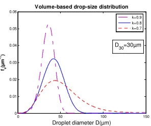
(76) We show as illustration in Fig. 10, the volume-based distributions fv(D), the different evolutions are in good agreement with literature results [31], [32].
0 50 100 150
0 0.01 0.02 0.03 0.04 0.05 0.06
Droplet diameter D(µm) fv
(µ
m
-1)
Volume-based drop-size distribution
k=0.9 k=0.8 k=0.7
[image:8.595.348.485.49.153.2]D30=30µm
Figure 10: Effect of kinetic energy on fv(D).
0 50 100 150
0 0.005 0.01 0.015 0.02 0.025 0.03 0.035 0.04
Droplet Diameter D(µm)
f(
µ
m
-1)
Number-based drop-size distribution
fn(D)
k=0.9
D30=30µm
Figure 11: Classical non-physical fn(D)distribution
Prediction with the generalized gamma distribution The previous method is limited by the fact its fn(D) lead to non physical result [31], [8] where drops of zero sizes seem to exists with a non-zero probability (Fig. 11). Whereas in [24] generalized gamma distribution give good results both for fn(D) and fv(D).
We use here the three-parameter generalized gamma distribution [24]
] ) ( exp[ )
( ) ( ) (
0 0
1
q q q
q n
D D q D
D q q q D
f α α
α α
α α
− Γ
=
− (77)
For this distribution, we have to determine the constraint diameter Dq0 and parameters of the Generalized Gamma α and q. We show in Fig. 12 this distribution in term of fn(D) and fv(D).
New physical approach for drop size distribution
Even if Generalized gamma distribution seems to fit well, there is a need to compute its parameters which has to link with the device generated the spray.
We propose a new approach allowing determining parameters Dq0 and q taking into account physical properties of the device. For that, our calculations are made thanks to the following relationship:
q n
q
q D f DdD
D 1/
0
0 [
∫
( ) ]∞
= (78)
Where fn(D) is given by (75) related to the physical properties of the SOD.
The resulting approach gives more realistic results. This new approach proposed takes into account the device properties and physical prediction possibility of Generalized Gamma drop size distribution, see in (Fig. 13) our coupling approach results.
0 50 100 150 200 250 300 350 0
0.01 0.02 0.03 0.04 0.05 0.06
Droplet Diamter D(µm)
Generalized-Gamma Distribution
fn fv
α=10; q=3;
[image:8.595.349.493.541.778.2]Dq0=100µm
Figure 12: Generalized gamma distribution
0 50 100 150
0 0.01 0.02 0.03 0.04 0.05 0.06
Droplet diameter D(µm)
fn
(µ
m
-1)
Number-based drop-size dristribution
k=0.7 (D
q0=28µm)
k=0.8 (Dq0=26µm)
k=0.9 (D
q0=24µm)
α=5 q=1.8 D
30=30µm
[image:8.595.91.239.637.760.2]V.CONCLUSION
In this work, we establish the theoretical relations describing the operation of the SOD. It takes into account the excitation applied to the PZA, the fluid flow in the tube up to spray generation via Faraday instability. We have started by establishing a general equation of motion of the tube thanks to Hamilton’s modified principle and taking into account non-linear effects such as the location of the PZA and other configurations of the SOD print-head during its operation. Analytical solutions are proposed for these equations in particular describing the transversal displacement of the tube conveying fluid subjected to an external pointwise excitation. The effect of fluid velocity on the transverse displacement of the tube is found to be negligible.
Our analysis leads us to:
1) The theoretical determination of volume and flow flux during the SOD operation, based on irreversible thermodynamics together with some assumptions on tube configurations.
2) The determination of an analytical expression for the Sauter Mean Diameter of the SOD according to the physical, mechanical and operational parameters the SOD. This analysis is based on the maximum entropy formalism (MEF) a widely used method which allows to choose among all the possible probability distributions the most suitable to the available knowledge on the phenomenon.
3) An innovative way of applying the MEF by combining the three-parameter generalized Gamma distribution with the physical based conservation laws method of MEF.
For a complete exploitation of the proposed model an identification of parameters is to be carried out in against experimental measurements. This allows proposing optimizations for the SOD with respect to its various potentials applications. Further work will be carried out to develop a multidisciplinary model.
VI. APPENDIX
Let us establish here the equation of motion of the nozzle conveying fluid in neglecting non-linear, gravity and PZA position effect.
Let Qr and M r
be the stress resultant and the couple resultant which the tube
and fluid on one side of a section at
s
exert on the other side (Fig. A).Figure A: sketch for fluid/tube equation of motion
A balance of forces gives:
) , ( ) ( ) , ( ) ,
( 2
2 2
t s r s U t t
t s r m j t x F s
Qr r r r
∂ ∂ + ∂ ∂ + ∂ ∂ = + ∂
∂ (A1)
A moment balance gives:
0
= × + ∂
∂ t Q
s
Mr r (A2)
With the Bernoulli-Euler hypothesis one has
s t t EI M
∂ ∂ × =
r r
r and
s M t Q
∂ ∂ × =
r r
r (A3)
We finally establish the fluid motion inside the SOD tube conveying fluid. It is more convenient to introduce dimensionless quantity, lengths are made dimensionless by dividing by L, but for convenience we continue to denote them by the same symbols.
, /L x
x= v=v/L, t=t/τ,finally, we obtain
) , ( 2 2 2 2 2 2 1 4 4
t x f x t
v c t
v x
v c x
v
= ∂ ∂
∂ + ∂ ∂ + ∂ ∂ + ∂
∂ (A4)
REFERENCES
[1] A.L. Yarin, Annual Review of Fluid Mechanics, January 2006, Vol.
38, Pages 159-192.
[2] C. Delattre, D. Vadillo and A. Soucemarianadin, Euromech
Colloquium 472, “Microfluidics and Transfer”, Grenoble, September 6 – 8, 2005.
[3] “Liquid Dispensing Apparatus, International Publication Number WO
99/46126, 16, September 1999. [4] http://www.flatjet-technology.com/
[5] M. Faraday, On the forms and states assumed by fluids in contact with vibrating elastic surfaces. Phil.Trans. R. Soc. Lond. 52, 319-340, 1831. [6] D. Sindayihebura , L. Bolle, A. Cornet ,L. Joannes , J. Acoust. Soc.
Am., vol. 103, No. 3, 1442-1448, 1997.
[7] R.J. Lang, Ultrasonic atomisation of liquids. J.Acoust.Soc.Am.34, 6-8, 1962.
[8] M. Dobre, Caractérisation stochastique des sprays ultrasoniques: le formalisme de l'entropie maximale, Thesis, UCL, 2003.
[9] http://www.americanpiezo.com/piezo_theory/index.html
[10] Piezoelectric Ceramics: Principles and Applications, by APC
International Ltd. ,ISBN-10: 0971874409, January 1, 2002
[11] M.P Paidoussis and N.T Issid, 1974, Sound Vib., 33(3), pp. 267–294.
[12] R.D. Blevins, 1977, Flow induced vibrations, New York: Van
Nostrand Reinhold.
[13] M.P. Païdoussis, C. Semler, M. Wadham-Gagnon & S. Saaid, Journal
of Fluids and Structures, 2007, 23, 569-587.
[14] G.W Housner, 1952, Journal of applied Mechanics 19,205-208.
[15] Y. H. Lin, C. L. Chu, Journal of sound and vibration, vol. 196, no1, pp. 97-105, 1996
[16] M. Wadham-Gagnon , M.P. Païdoussis, and C. Semler, Journal of
Fluids and Structures Volume 23, Issue 4, May 2007, pp. 545-567
[17] D. S. Weaver and T. E. Unny, Journal of Applied Mechanics 40, 48-52
(1973)
[18] T. Brooke Benjamin, Proceedings of the Royal Society of London, Vol.
261, pp. 457-486, 1961.
[19] T.S Lundgren, P.R. Sethna, A.K Bajaj, Journal of Sound and
Vibration, Volume 64, Issue 4, p. 553-571, 1979
[20] S. Middleman, Modeling Axisymmetric Flows, Academic Press
(1995)
[21] C.E. Shannon,Key papers in the development of information theory, Bell Syst. Tech. J., vol. 27, p.623-656, 1948.
[22] Y. Agmon , N.Alhassid and R.D. Levine, J. of Comp. Phys., vol. 30,
N°2, p. 250-258, 1977
[23] R.W. Sellens, Drop size and velocity distribution in sprays. A new approach based on the maximum entropy formalism, Ph.D thesis, Univ. of Waterloo, 1987.
[24] C. Dumouchel , Part. Part. Syst. Charact. 23 (2006) 468–479
[25] R. W. Sellens, T. A. Brzustowski, Atomization and Spray Technology
1985, 1, 89–102.
[26] X. Li and R.S Tankin , Comb. Sci. Technol., vol.60, p 345-357, 1988.
[27] Van 1994] C.W.M Van der Geld and H. Vermeer , Int. J. Multiphase
Flow, vol.20, n°2, p.363-381, 1994.
[28] C.H. Yau. , A.K. Bajaj, O.D.I. Nwokah, Journal of fluids and
structures, vol. 9, no1, pp. 99-122,1995
[29] I. Prigogine, D. Kondepudi, Thermodynamique: Des moteurs
thermiques aux structures dissipatives, Sciences, Odile Jacob, 1999
[30] I. Prigogine, D. Kondepudi, Modern Thermodynamics: From Heat
Engines to Dissipative Structures, John Wiley & Sons, 1998
[31] E. Babinski, P. E. Sojka, Progress in Energy and Combustion Science
2002, 28, 303–329.
[32] M.Dobre, L. Bolle, Theoretical prediction of ultrasonic spray
characteristics using the maximum entropy formalism.