Abstract— This paper presents research on the Vehicle Routing Problem (VRP) using a sweep heuristic method with 2-opt exchange and traveling salesman tours and an integer programming model for split delivery VRP model to select the best route to pick up and delivery customers from/to desired destination and depot. The modeling language, AMPL with CPLEX is used to develop the model and implement the sweep heuristic. The research found that the integer programming model produced the optimal result for some cases and failed to produce the optimal result for some cases. However, the sweep heuristic gave good solutions for all cases within a small amount of computational time. The research also investigated sensitivity analysis with respect to the vehicle capacity. The results indicate a savings in number of vehicle used with a small increase in vehicle capacity. The case study of University of The Thai Chamber of Commerce (UTCC) which provides bus services to pick up and deliver staff from/to home and university is selected to present in this paper.
Index Terms— Vehicle Routing Problem (VRP), Sweep Heuristics Method, Integer Programming Model, Split Delivery VRP Model
I. INTRODUCTION
The Vehicle Routing Problem (VRP) is a well-known problem studied by researchers in different areas such as Operations Research, Decision Support Systems, and Artificial Intelligence. The VRP deals with distribution of goods from a depot to a set of customers in a given time period by a fleet of vehicles which are operated by a set of drivers who perform movements on an appropriate road network. The solution of a VRP is a set of minimum cost routes, which satisfy the problem’s constraints, and fulfill customers’ requirements.
In the VRP, the road network is represented by a graph with arcs and vertices. Arcs represent roads and vertices represent road intersections, junctions, customer locations, and the depot. Each arc has an associated cost. Each customer location vertex has an associated number of goods to be delivered. Every vehicle has its own capacity and cost associated with its utilization. There are objectives other than minimizing the transportation cost that may arise in vehicle routing problems such as minimizing the number of vehicles required to serve all customers, balancing the routes, or minimizing a penalty associated with partial service of the customers.
The VRP may be defined mathematically as follows. Let
Manuscript received December 11, 2007. This work was supported by the University of the Thai Chamber of Commerce.
Nanthi Suthikarnnarunai is with the Department of Logistics, School of Engineering, University of the Thai Chamber of Commerce, Bangkok,
Thailand (phone & fax: 662-2754892); e-mail: [email protected],
G = (V, A) be a network where V = {0, 1, … , n} is the vertex set and A⊆V×V is the arc set. Vertex 0 is the depot and V\{0}
is the set of customer locations on the road network. Associated with vertex i ∈V\{0} is a non-negative demand di. The parameter cij represents a non-negative cost or distance between vertices i and j. The parameters K and Uk are the number of vehicles and the capacity of vehicle k, respectively. Reference [1] describes the VRP with an integer programming formulation using a three-index vehicle flow formulation where binary variables xijk count the number of times arc (i,j)∈A is traversed by vehicle k (k = 1,…,K) in the optimal solution . In addition, there are binary variables yik (i∈V; k = 1,…,K) that take a value of 1 if vertex
i is visited by vehicle k in the optimal solution and take a value of 0, otherwise. The formulation is as follows:
min
∑ ∑
∈A = j i
K
k ijk ij
x
c
) ,
( 1
(1) subject to
∑
=∈
∀
=
K
k
ik
i
V
y
1
}
0
{
\
1
(2)
∑
==
K
k
k
K
y
1
0 (3)
x
y
iki
V
k
K
i V j
ijk
,
1
,...,
}{ \
=
∈
∀
=
∑
∈(4)
∑
∈
=
∈
∀
=
} { \
,...,
1
,
i V j
ik
jik
y
i
V
k
K
x
(5)
∑
∈=
∀
≤
} 0 { \
,...,
1
V i
k ik
i
y
U
k
K
d
(6)K
k
S
V
S
S
x
S i jS i
ijk
1
\
{
0
},
2
,
1
,...,
}{ \
=
≥
⊆
∀
−
≤
∑ ∑
∈ ∈(7)
y
ik∈
{
0
,
1
}
∀
i
∈
V
,
k
=
1
,...,
K
(8)x
ijk∈
{
0
,
1
}
∀
(
i
,
j
)
∈
A
,
k
=
1
,...,
K
(9) Constraints (2) - (5) ensure that each customer is visited exactly once, that K vehicles leave the depot, and that the same vehicle enters and leaves a given customer vertex, respectively. Constraints (6) are the capacity restrictions for each vehicle k, whereas constraints (7) are sub-tour elimination constraints for each vehicle. Note that in (7), S is a subset of the stops that does not contain the depot. Three-index vehicle flow models have been extensively used to model more constrained versions of the VRP, such as the VRP with time windows (VRPTW).The VRP is an NP-hard problem [2], and so it is difficult to solve. There are many variations on the basic VRP as stated above such as the traveling salesman problem (TSP), the arc routing problem, and the VRP with time windows. Each type
A Sweep Algorithm for the Mix Fleet Vehicle
Routing Problem
of problem has its own characteristics.
The capacitated VRP (CVRP) is a problem in which all customer demand must be satisfied, all demands are known, all vehicles have identical, limited capacity and are based at a central depot. The objective of CVRP is to minimize total transportation cost or time [1]. The VRPTW is an extension of CVRP with a time constraint for reaching each customer [1]. The service can be performed only within a specified time interval. A vehicle is permitted to arrive before the opening of the time window, but must wait, at no cost, until service becomes possible. Arrival after the latest time window is not permitted [3].
The VRP with backhauls (VRPB) is a VRP with customers separated into two groups – linehaul customers who are demanding goods and backhaul customers who are returning goods. The operations of this problem must be delivery first and pick up later (i.e., linehaul first and backhaul later). The objective of VRPB is to find a set of routes that minimizes the total cost, time, or distance traveled [1].
The VRP with pickup and delivery (VRPPD) requires delivery of goods to the customers at one location and then picking up other types of goods from them to be brought back to the depot. The objective of VRPPD is to minimize the vehicle fleet size and total cost/time/distance traveled [1].
In the split delivery VRP (SDVRP), customers at each point may be served by different vehicles. This is necessary if the requirement at any customer vertex exceeds the vehicle capacity [4]. The fleet size and mix VRP (FSMVRP) or vehicle fleet mix problem is another variant of VRP in which the vehicles have different capacities, different fixed costs, and different variable costs [5].
II. SURVEY OF VRP LITERATURE
VRP was first studied by [6]. Since then, there have been many VRP studies reported in the literature. References [7], [8], and [9] apply VRP models to school bus routing. Other applications include inventory and vehicle routing in the beverage, food, and dairy industries, distribution and routing in the newspaper industry [10], railroad industry [11], transit bus services [12], grass mowing industry [13], public library systems [14], post service [15], and grocery delivery [16]. More comprehensive surveys of the VRP literature may be found in [4], [12],[17], [18], and [19].
VRP solution methods fall into two main categories: exact methods and heuristics. Branch-and-bound and branch-and-cut, are both exact methods which have been proposed for VRP by many researchers such as [1], [20], [21], [22], and [23].
Heuristics are methods which produce good solutions in practice but do not guarantee optimality. Reference [1] defines classical heuristics as methods which quickly provide good solutions by limiting the search space. Classical heuristics fall into three subcategories: constructive heuristics, two-phase heuristics, and improvement methods. Examples of classical VRP heuristics in the literature include [5], [24], [25], [26], and [27]. Metaheuristics give better solutions than classical heuristics, but consume more computational time. Some of the most popular metaheuristics are simulated annealing (SA), deterministic annealing (DA), tabu search (TS), generic algorithms (GA), ant systems (AS), constraint programming, and neural networks (NN).
Several researchers use SA to solve VRPTW such as [13] and [28]. Applications of TS to VRP include [29], [30], and [31]. References [32], [33], and [34] apply GA to solve VRP. References [35], [36], and [37] use AS to solve VRP. A constraint programming method for VRP has been proposed by [38]. Neural Networks for VRP are mostly used in combination with other methods to solve the problem. For example, [39] used NN together with AS to solve VRPTW. Reference [40] used NN and GA to solve the multi-depot vehicle routing problem.
III. A VRP CASE STUDY OF UTCC’S BUS SERVICE University of the Thai Chamber of Commerce (UTCC) is a private non-profit higher education institution in Bangkok offering degrees in Business Administration, Accountancy, Economics, Humanities, Science, Communication Arts, Engineering, and Law. Currently, the UTCC provides bus services to pick up and deliver staff from/to home and university in the morning and evening periods. There are 4 routes currently in service and each route has been established by an intuitive method. A recent survey of UTCC bus riders revealed widespread dissatisfaction with the service. Riders complained about the limited number of routes, stops, and vehicles.
UTCC currently has a fleet of 12 vehicles of which 4 are used to service these customers. These 12 vehicles consist of 2 Scania buses with a capacity of 40 seats each, 2 BMC buses with a capacity of 30 seats each, and 8 vans with a capacity of 12 seats each. The buses may not be available on any given day since they are used in other university operations, but at least 4 vans are available everyday. The following is the list of assumptions that shaped our formulation of the VRP model for UTCC:
• Each route will start from and end at UTCC.
• The cost of a route is proportional to the time traveled.
• Travel times between each stop are known and accurate.
• Demands (i.e., number of passengers) at each of the stops are known.
• The demand at each stop can be split. That is, multiple vehicles may be used to pickup passengers at any given stop.
• Loading time per passenger is constant for every passenger.
The constraints in this problem are:
• The capacity of the vehicles is strictly enforced, a customer may not stand up on the vehicle.
• Hour of operations – there is a time window for delivering passengers to UTCC in the morning and evening.
In the case of UTCC, in which the demand at each stop can be split, the binary variable
y
ik is replaced with the integer variablez
ik(i ∈ V; k = 1,…,K), which indicates the number of passengers at stop i that are picked up by vehicle K. We use a loading time of 6 seconds (0.1 minute) per passenger as recommended in the literature [41]. The parameter t is the time window. Therefore, the equations (2) – (6) and equation (8) must be dropped and the following equations will be added:∑
==
K
k
i ik
d
z
1
∑
∈≤
V i
k
ik
U
z
k
=
1
,...,
K
(11)∑
∈
≤
} \{i V j
ijk i
ik
d
x
z
∀
i
∈
V
,
k
=
1
,...,
K
(12)∑
∑
∈ ∈
=
} {
\i \{} V
j jV i
jik
ijk
x
x
∀
i
∈
V
,
k
=
1
,...,
K
(13)1
} 0 { \
0
=
∑
∈V jjk
x
k
=
1
,...,
K
(14)∑
∑
∑
∈ = ∈
≤
+
A j
i iV
ik K
k ijk
ij
x
z
t
c
) ,
( 1
1
.
0
k
=
1
,...,
K
(15) Constraints (10) and (11) ensure that the passengers at all stops will be picked up and the capacity restriction for each vehicle k is enforced, respectively. Variablesx
ijkandz
ikare linked by constraint (12). Constraint (13) is the flow balance constraint which means the same vehicle enters and leaves a given customer vertex. Constraint (14) shows that all vehicles must start at the depot. The time window constraints are (15), where t is 150 minutes for the morning run and 180 minutes for the evening run. The travel time is (2.1) plus 0.1 times the total demandThe overall goal of this research is to develop a plan for the university’s bus service to be able to serve all customers in the most efficient way. New and improved sets of routes are created with all possible fleet configurations as following.
1. Only vans are available.
2. 1 Scania bus and 8 vans are available. 3. 2 Scania buses and 8 vans are available. 4. 1 BMC bus and 8 vans are available. 5. 2 BMC buses and 8 vans are available.
6. 1 Scania bus, 1 BMC bus, and 8 vans are available. 7. 2 Scania buses, 1 BMC bus, and 8 vans are available. 8. 1 Scania bus, 2 BMC buses, and 8 vans are available. 9. 2 Scania buses, 2 BMC buses, and 8 vans are available.
IV. A DECOMPOSITION ALGORITHM FOR VRP As mentioned earlier, there are many methods used to solve VRP problems, the idea of cluster first and route second had been employed in this research. The sweep algorithm was used for clustering, while traveling salesman tours were used to order the stops in the clusters found by the sweep. In some cases, 2-opt exchanges was used to adjust the clusters, resulting in improved solutions. The following is the description of the decomposition algorithm for our problem. A. Sweep Algorithm
The sweep algorithm is a method for clustering customers into groups so that customers in the same group are geographically close together and can be served by the same vehicle. The sweep algorithm uses the following steps.
1. Locate the depot as the center of the two-dimensional plane.
2. Compute the polar coordinates of each customer with respect to the depot.
3. Start sweeping all customers by increasing polar angle. 4. Assign each customer encompassed by the sweep to the
current cluster.
5. Stop the sweep when adding the next customer would violate the maximum vehicle capacity.
6. Create a new cluster by resuming the sweep where the last one left off.
7. Repeat steps 4 – 6, until all customers have been included in a cluster.
In our case, the demand at some stops may exceed the capacity of the vehicles. The modification to the sweep algorithm that we have made for this specific case study is to add the preprocessing step. In general, if any stop has demand greater than or equal to the capacity of the vehicle, then we assign a vehicle to pick up customers at that stop in the amount equal to the capacity of the vehicle and leave the rest of the demand for the regular sweep steps.
From the characteristics of the problem there are several cases that might happen when there is a mix of vehicle types in the fleet. When we have a mixed fleet, we need to do the sweep more than one time to get the result. The general steps of solving a mixed fleet model by using the sweep algorithm are as follows.
1. Start the first sweep by using the highest vehicle capacity in the fleet as the capacity limitation.
2. From the result, choose the route with the highest number of customers as part of our solution, and then discard the data of all stops in our chosen route. 3. Do the next sweep by using the next highest vehicle
capacity in the fleet as the capacity limitation.
4. Repeat steps 2 and 3 until all vehicle sizes have been considered or there are no customers left.
B. Traveling Salesman
The famous traveling salesman problem, is solved to route the shortest tour in each cluster in the second phase. The TSP is known as the method used to find the cheapest way of visiting all of a given set of cities and returning to the starting point. The cheapest way may refer to cost, distance or time of traveling in each route. Since the clusters in the UTCC problem are relatively small, we solve the resulting TSP instances with a straightforward integer programming model.
C. 2-Opt Exchange
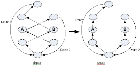
[image:3.612.78.294.50.181.2]The 2-opt exchange is a method for exchanging two groups of customers in different routes, resulting in lower mileage, cost, or time in each route. The process will be repeated until no more exchanges produce a decrease in mileage, cost, or time. This will result in a new set of clusters. Reference [42] shows what two routes would look like after performing a 2-opt exchange as in Figure 1.
Figure 1 2-opt Exchange Swapping Customers A and B
V. INITIAL RESULTS
[image:3.612.314.539.557.662.2]columns: the vehicle used, route, total number of passengers in each vehicle, and total time used by the vehicle. The table shows the stops by order received from the TSP algorithm, along with the number of passengers picked up at each stop. We use the notation “L(N)”, in which L refers to the stop location and N refers to the number of customers that will be picked up at stop L. For example, “4(6)” means 6 people will be picked up at stop number 4.
0 2 4 6 -6 -4 -2 8 10 12 14 16 18 20 0 2 4 6 -6 -4 -2 8 10 12 14 16 18 20
0 2 4 6 8 10 12
-2 -4 -6 -8 -10 -12
0 2 4 6 8 10 12
-2 -4 -6 -8 -10 -12 AM1 (1) D=4 AM2 (2) D=1 AM3 (3) D=1 AM4 (4) D=1 BM1 (5) D=2 BM2 (6) D=13 BM3 (7) D=8 CM1 (8) D=3 CM2 (9) D=2 CM3 (10) D=2 CM4 (11) D=4 CM5 (12) D=3 CM6 (13) D=9 DM1 (16) D=5 DM2 (15) D=2 DM3 (14) D=6 DM4 (17) D=2 DM5 (19) D=4 DM6 (18) D=3 DM7 (20) D=13 DM8 (21) D=4 UTTC (Depot) = VAN[1] = VAN[2] = VAN[3] = VAN[4] = VAN[5] = VAN[6] = VAN[7] = VAN[8] = VAN[9]
Figure 2 Vans-Only Morning Run
Table 1 Vans-Only Morning Run
VI. EXACT METHODS
Exact methods for solving VRP are quite limited, because of the combinatorial explosion [43]. Many successful heuristic methods have been developed to solve VRP. In our investigation, a heuristic composed of the sweep method, traveling salesman tours, and 2-opt exchanges has been selected to solve our problem. The results of the heuristic in the van-only case, 9 vans are required for serving all customers in the morning run. The total travel time in the solution from the heuristic is 822.2 minutes. This result was obtained on a Pentium 4 PC with 512 MB of RAM in about 3 seconds of computational time.
For the exact method, we replaced constraint (7) with the following equation
∑ ∑
′ ∈ ∈ ′−
′
≤
S i j S iijk
S
x
} \{
1
∀
S
′
,
k
=
1
,...,
K
(16) whereS
′
is a given set of subtours. Then, we implemented a subtour generation procedure for VRP as follows:1. Let
S
′
=
φ
.2. Solve model (10) – (16). 3. Check the solution for subtours.
4. If any subtours are found, add them to
S
′
and go to step 2.5. Stop, current solution is optimal.
The best solution received from the solving method mentioned above is to use 8 vans to serve all customers in the morning run. There are 3,696 binary variables, 176 integer variables and 3,757 constraints in the IP model when
φ
=
′
S
. The IP model was too large to solve on the PC used to obtain the results in Appendix A. To solve it, we used a Dell PE 2650 with 4,096 MB of RAM and dual Intel Xeon processors running at 3.0 GHz. The total travel time in the IP solution is 776.2 minutes with a 10% optimality gap. The computational time using AMPL with CPLEX 10.0 was 35,109.07 seconds which is almost 10 hours. If 9 vans are used in the exact method, the total travel time with a 10% MIP gap is 749.2 minutes. The computational time for the latter case was 11,418.25 seconds (3.17 hours). This shows that the results received from our heuristic are good enough compared to the results from the exact method, and that the heuristic uses considerably less computational time and memory. Figures 3 and 4 show the routes produced by the exact method using 8 vans and 9 vans, respectively.0 2 4 6 -6 -4 -2 8 10 12 14 16 18 20 0 2 4 6 -6 -4 -2 8 10 12 14 16 18 20
0 2 4 6 8 10 12
-2 -4 -6 -8 -10 -12
0 2 4 6 8 10 12
-2 -4 -6 -8 -10 -12 AM1 (1) D=4 AM2 (2) D=1 AM3 (3) D=1 AM4 (4) D=1 BM1 (5) D=2 BM2 (6) D=13 BM3 (7) D=8 CM1 (8) D=3 CM2 (9) D=2 CM3 (10) D=2 CM4 (11) D=4 CM5 (12) D=3 CM6 (13) D=9 DM1 (16) D=5 DM2 (15) D=2 DM3 (14) D=6 DM4 (17) D=2 DM5 (19) D=4 DM6 (18) D=3 DM7 (20) D=13 DM8 (21) D=4 UTTC (Depot) = VAN[1] = VAN[2] = VAN[3] = VAN[4] = VAN[5] = VAN[6] = VAN[7] = VAN[8]
Figure 3 Exact Method Result: 8 Vans Morning Run
Table 2 Recommended Van Capacity to all cases
[image:4.612.70.299.134.544.2] [image:4.612.312.544.321.697.2]seconds (1 hour) in each subtour elimination iteration (steps 2 – 4). We tried to increase the processing time per iteration to 15,000 seconds but the program terminated before finding a feasible solution (i.e., it never got to step 5). Therefore, we used another program to generate the subtour elimination constraints for all subtours with 5 or fewer stops before solving the model. This gave us 75,777 subtours. This process took one day of CPU time. When we solved this model, the best solution we got had a 19.17% optimality gap with a total travel time of 714.7 minutes for the van-only case (This solution was obtained using a van capacity of 17 during the sensitivity analysis described in section 7). The computational time was 74.67 hours. While we got the total travel time of 1,063.7 minutes from the sweep method, with the computational time of 16 seconds. However, we obtain results of all cases from the sweep method. In the evening run, both sweep and exact procedure was too large to solve on the PC, and so we used a Dell PE 2650 with 4,096 MB of RAM and dual Intel Xeon processors running at 3.0 GHz is used to run the algorithm.
0 2 4 6
-6 -4 -2 8 10 12 14 16 18 20
0 2 4 6
-6 -4 -2 8 10 12 14 16 18 20
0 2 4 6 8 10 12
-2 -4 -6 -8 -10 -12
0 2 4 6 8 10 12
-2 -4 -6 -8 -10 -12
AM1 (1) D=4 AM2
(2) D=1 AM3
(3) D=1 AM4
(4) D=1
BM1 (5) D=2
BM2 (6) D=13
BM3 (7) D=8 CM1
(8) D=3
CM2 (9) D=2 CM3 (10) D=2
CM4 (11) D=4 CM5 (12) D=3
CM6 (13) D=9
DM1 (16) D=5
DM2 (15) D=2
DM3 (14) D=6
DM4 (17) D=2 DM5
(19) D=4
DM6 (18) D=3
DM7 (20) D=13
DM8 (21) D=4
UTTC (Depot) = VAN[1]
= VAN[2]
= VAN[3] = VAN[4]
= VAN[5]
= VAN[6]
= VAN[7] = VAN[8]
= VAN[9]
Figure 4 Exact Method Result: 9 Vans Morning Run
VII. SENSITIVITY ANALYSIS FOR UTCC’S BUS SERVICE
In this section, we present alternative solutions for UTCC’s bus service. Sensitivity analysis gives alternative solutions in accordance to changes in vehicle capacity. Considering UTCC’s current operations and the size of Thai people, we saw that the capacity of the buses and vans may be expanded. The vans may be able to load up to 17 people and 10 more customers may be allowed to stand on the bus when the seats are full. The sweep results when we assigned the bus capacity a large number (capacity of 60) reveal that no matter how much extra capacity we assigned to the buses, the number of customers that the Scania bus can pick up under our time constraint will not exceed our current maximum capacity of 40 seats. Therefore, our sensitivity analysis is
only performed on the van capacity. In case of the BMC bus, we can use the solution with the Scania bus if we allow customers to stand on the bus. The results reveal that in most of the cases, the more capacity of the van, the less number of vehicles required. Table 2 is our recommendation to UTCC for every case we mentioned in section 3, considering the comfort of the customer.
VIII. SUMMARY AND RECOMMENDATION From the organized of this paper, several tasks have been accomplished. A comprehensive literature review is reported in section 2. The sweep method followed by the traveling salesman, and 2-opt exchange has been implemented to solve all cases of our problem. An exact method using integer programming has been applied to the van-only morning run case. The modeling language for mathematical programming called AMPL has been used for this propose. Also, the sensitivity analysis option for UTCC have been purposed in section VII. This section presents a
recommendation to UTCC for a cost effective way to implement new routes given UTCC’s current resources, and also to make a recommendation for expanding the service in the future. The recommendation about the future research in the area of VRP is also mentioned in this section.
One interesting option for UTCC’s service is not to start vehicles at the depot. Our method for this idea is to find routes in the morning in which the first stop in each route is not at the depot. Then, the vehicles will pick up customers at other stops along the route and end at the depot, while not exceed the vehicle capacity and the time limit of 150 minutes. In the evening run, all the vehicles will start at the depot, drop the customers at their stops, and end the routes at the stops which are the starting stops in the morning. If the evening run uses more vehicles than the morning run, the extra vehicles must go back to the depot. However, in both cases, all routes must be created under the objective function of minimizing the total travel time of all vehicles.
sweep method.
REFERENCES
[1] Toth, P., & Vigo, D. (2002). The Vehicle Routing Problem. SIAM,
Philadelphia.
[2] Machado, P., Tavares, J., Pereira, F., & Costa, E. (2002). Vehicle
Routing Problem: Doing it the Evolutionary Way. Proceedings of the
Genetic and Evolutionary
Computation Conference (GECCO'2002), 690
[3] Bräysy, O., & Gendreau, M. (2005). Vehicle Routing Problem with Time Windows, Part I: Route Construction and Local Search Algorithms.
Transportation Science, 39(1), 104-118.
[4] Díaz, B.D. VRP Web. Retrieved October, 2005, from
http://neo.lcc.uma.es/radiaeb/WebVRP.
[5] Renaud, J. & Boctor, F. (2002). A Sweep Based Algorithm for the Fleet
Size and Mix Vehicle Routing Problem. European Journal of Operational
Research, 140, 618-628.
[6] Dantzig, G.B. & Ramser, J.H. (1959). The Truck Dispatching Problem.
Management Science, 6, 80-91.
[7] Bowerman, B., Hall, B., & Calamai, P. (1995). A Multiobjective Optimization Approach to Urban School Bus Routing: Formulation and
Solution Method. Transportation Research - Part A, 29A, 107-123.
[8] Kelnhofer-Feeley, C., Hu, Q., Chien, S., Spasovic, L., & Wang, Y. (2001). A Methodology for Evaluating of School Bus Routing: A Case Study
of Riverdale, New Jersey. Transportation Research Board 80th
Annual Meeting, Washington DC, January 2001.
[9] Thangiah, S., Wilson, B., Pitluga, A. & Mennell, W. (2004). School Bus Routing in Rural School Districts. Working Paper. Artificial Intelligence and Robotics Lab. Computer Science Department, Slippery Rock University, Slippery Rock, PA.
[10] Golden, B., Assad, A., & Wasil, E. (2002). Routing Vehicles in the Real World: Applications in the Solid Waste, Beverage, Food, Dairy, and Newspaper Industries. In The Vehicle Routing Problem, Toth, P. and Vigo, D. (eds), SIAM Monographs on Discrete Mathematics and Applications, Philadelphia, 245-286.
[11] Lübbecke, M. & Zimmermann, U. (2003). Engine Routing and
Scheduling at Industrial In-Plant Railroads. Transportation Science, 37(2),
183–197.
[12] Nurcahyo, G., Alias, R., Shamsuddin, S., & Sap, M. (2002). Vehicle
Routing Problem For Public Transport : A Case Study. Proceedings of the
2002 International Technical Conference On Circuits/Systems, Computers and Communications, Phuket, Thailand, 1180-1183.
[13] Stewart, P. & Tipping, J. (2002). Scheduling and Routing Grass
Mowers Around Christchurch. 37th
Annual ORSNZ Conference, University of Auckland, NZ, November 2002.
[14] Foulds, L., Wallace, S., Wilson, J., & Sagvolden, L. (2001). Bookmobile Routing and Scheduling in Buskerud County, Norway.
Proceedings of the 36th Annual Conference of the Operational Research Society of New Zealand, Christchurch, New Zealand, December 2001, 67-77. [15] Rodrigues, A., & Ferreira, J. (2001). Solving the Rural Postman
Problem by Memetic Algorithms. Proceeding of MIC’2001 – 4th
Metaheuristics International Conference, Porto, Portugal, July 16-20, 2001. [16] Bürchett, D. & Campion, E. (2002). Mix Fleet Vehicle Routing Problem - An Application of Tabu Search in the Grocery Delivery Industry. Research Paper, University of Canterbury, New Zealand.
[17] Laporte, G. (1992). The Vehicle Routing Problem: An Overview of
Exact and Approximate Algorithms. European Journal of Operational
Research, 59, 345-358.
[18] Ball, M., Magnanti, T., Monma, C., & Nemhauser, G. (1995). Handbooks in Operations Research and Management Science. V.8., Elsevier Science, The Netherlands.
[19] Laporte, G. & Osman I. H. (1995). Routing Problems: A Bibliography.
Annals of Operations Research, 61, 227-262.
[20] Fisher, M. (1994). Optimal Solution of Vehicle Routing Problems
Using Minimum K-trees. Operations Research, 42, 626-642.
[21] Lee, E., & Mitchell, J.(1998). Branch-and-Bound Methods for Integer
Programming. The Encyclopedia of Optimization, Kluwer Academic
Publishers.
[22] Brad, J., Kontoravdis, G., & Yu, G. (2002). A Branch-and-Cut Procedure for the Vehicle Routing Problem with Time Windows.
Transportation Science, 36(2), 250-269.
[23] Ortega, F., & Wolsey, L. (2003). A Branch-and-Cut Algorithm for the Single-Commodity, Uncapacitated, Fixed-Charge Network Flow Problem.
Networks, 41(3), 143-158.
[24] Clarke, G. & Wright, J. (1964). Scheduling of Vehicles from a Central
Depot to a Number of Delivery Points, Operations Research, 12(4), 568-581.
[25] Gillett, B. & Miller L. (1974). A Heuristic for the Vehicle Dispatching
Problem. Operations Research, 22, 340-349.
[26] Fisher, M. & Jaikumar, M. (1981). A Generalized Assignment Heuristic
for Vehicle Routing, Networks, 11, 109-124.
[27] Ryan, D., Hjorring C. & Glover F. (1993). Extension of the Petal
Method for Vehicle Routing. Journal of the Operational Research Society,
44, 289-296.
[28] Czech, Z., & Czarnas, P. (2002). Parallel Simulated Annealing for the
Vehicle Routing Problem with Time Windows. 10th Euromicro Workshop
on Parallel, Distributed and Network-based Processing, Canary Islands - Spain, 376-383, January 9-11, 2002.
[29] Thangiah, S., Osman, I., & Sun, T. (1994). Hybrid Genetic Algorithm Simulated Annealing and Tabu Search Methods for Vehicle Routing Problem with Time Windows. Technical Report 27, Computer Science Department, Slippery Rock University, 1994.
[30] Toth, P., & Vigo, D. (1998). The Granular Tabu Search and its Application to the Vehicle Routing Problem. Working Paper, DEIS, University of Bologna.
[31] Bräysy, O., & Gendreau, M. (2003). Metaheuristic Approaches for the
Vehicle Routing Problem with Time Windows: A Survey. Proceeding of
MIC’2003 – 5th
Metaheuristics International Conference, , Kyoto, Japan, August 25-28, 2003.
[32] Berger, J., Barkaoui, M., & Bräysy, O. (2001). A Parallel Hybrid Genetic Algorithm for the Vehicle Routing Problem with Time Windows. Working paper, Defense Research Establishment Valcartier, Canada. [33] Bräysy, O. & Gendreau, M. (2001). Genetic Algorithms for the Vehicle Routing Problem with Time Windows. Internal Report STF42 A01021, SINTEF Applied Mathematics, Department of Optimization, Oslo, Norway. [34] Jih, W. & Hsu, J. (1999). Dynamic Vehicle Routing Using Hybrid
Genetic Algorithms. Proceedings of the 1999 IEEE International Conference
on Robotics & Automation, Detroit, Michigan. May 1999.
[35] Bullnheimer, B., Hartl, R., & Strauss, C. (1997). Applying the Ant System to the Vehicle Routing Problem. Paper presented at 2nd International Conference on Metaheuristics, Sophia-Antipolis, France.
[36] Gambardella, L., Taillard, E., & Agazzi, G. (1999). MACS-VRPTW: A Multiple Ant Colony System for Vehicle Routing Problems with Time
Windows. In D. Corne, M. Dorigo and F. Glover, editors, New Ideas in
Optimization. McGraw-Hill.
[37] Reimann, M., Doerner, K., & Hartl, R. (2003). Analyzing a Unified Ant System for the VRP and Some of Its Variants. S. Cagnoni et al. (Eds.):
EvoWorkshops Springer-Verlag Berlin Heidelberg 2003, LNCS 2611, 300–310.
[38] Shaw, P. (1998). Using Constraint Programming and Local Search
Methods to Solve Vehicle Routing Problems. Proceedings of the Fourth
International Conference on Principles and Practice of Constraint Programming (CP '98), M. Maher and J.-F. Puget (eds.), Springer-Verlag, 417-431.
[39] Barán, B. & Schaerer, M. (2003). A Multiobjective Ant Colony System
for Vehicle Routing Problem with Time Windows. Proceedings of the 21st
IASTED International Conference on Applied Informatics, IASTED, Innsbruck, Austria, February 2003, 97-102.
[40] Salhi, S., Thangiah, S., & Rahman, F. (1998). A Genetic Clustering
Method for the Multi-Depot Vehicle Routing Problem. Artificial Neural
Network and Genetic Algorithms, (GD Smith, NC Steel and RF Albrecht (Eds)), Springer, NY, 234-237.
[41] Christchurch City Council. (2006). Transportation Service Project. [42] Restori, M. (2004). An Application of VRP Algorithms with Original Modifications.
Presented Paper at the IIE international conference in Houston, TX in May, 2004.