II.T HE IDEF0 FUNCTION

Abstract—Aggregate Production Planning (APP) is a medium term Planning that links between the long term planning and the short range planning. Although there are many models developed by the researchers in this area, few of them are being implemented. This reason was the motive to develop a model in a different way than the traditional models used to be developed. The Integrated Definition level 0 (IDEF0) is used in this paper to represent the development of a typical APP model. The IDEF0 shows the model formulation using goal programming (GP) including identification of the model goals and model constraints, preparation of the model format, and finally solution of the model using a Genetic Algorithm (GA) approach. The IDEF0 as a structured methodology enhances the model development process, and make the relationships between the objective function and constraints crystal pure, which in consequences enhances the problem representation and solution procedure.

Index Terms—Aggregate production planning, genetic algorithm, goal programming, integrated definition, system analysis.

I. INTRODUCTION

Aggregate production planning (APP) deals with matching capacity to demand over a period that varies from three to eighteen months. It aims at setting overall production levels for each product family, and to set decisions and policies concerning workforce level, hiring, layoffs, overtime, backorders, subcontracting, and stock level. It has received much attention in literature where it is addressed under diverse names such as APP, workforce planning, production and employment smoothing, capacity and production planning [1]. Furthermore, APP is an important problem due to the fact that the APP approach has a direct effect on the profitability and objectives of a company [2].

This paper describes the development of a typical APP model, which is modeled as a multi-objective goal programming model and solved with genetics algorithm [3], using a structured system analysis methodology.

Manuscript received January 7, 2008.

Mootaz M. Ghazy is a Ph. D. research student, and is an assistant lecturer at the Department of Industrial and Management Engineering, College of Engineering and Technology, Arab Academy for Science and Technology, Abu Keer Campus, P.O. Box 1029, Alexandria, Egypt (e-mail: [email protected]).

Khaled S. El-Kilany, Ph. D., is an Assistant Professor at the Department of Industrial and Management Engineering, College of Engineering and Technology, Arab Academy for Science and Technology, Abu Keer Campus, P.O. Box 1029, Alexandria, Egypt (e-mail: [email protected]).

M. Nashaat Fors, Ph. D., is a Professor of Industrial Engineering, Production Engineering Department, Faculty of Engineering, Alexandria University (e-mail: [email protected]).

The motive to using this methodology is the fact that the different the APP problem involves multiple objectives, which are conflicting in nature. The conflict arises because improvement in one objective may be made at the expense of one or more of the remaining objectives. Consequently, the systems approach is applicable in this situation to identify the different interactions between these objectives and how they are affected by afore mentioned decisions and policies.

In context of a typical aggregate production planning problem, examples of the multiple objectives can be [4]: maximizing profit or minimizing costs, minimizing amount of inventory, minimizing backorders or shortages, maintaining a balanced labor force, maximizing the utilization of the facilities, and minimizing the use of overtime.

The paper starts with a brief introduction to the system analysis methodology used to model the development of the APP model, which is the IDEF0 modeling method. Then, the model basic idea including the functions considered and their level of details are presented. Afterwards, each function and their inter-relationships are fully described. Finally, the conclusions drawn from this work are pointed out.

II. THE IDEF0FUNCTION MODELING METHOD

IDEF is an Integration computer-aided manufacturing DEFinition language that consists of a set of re-engineering techniques developed by the Air Force to facilitate manufacturing automation [5].

Following structured system analysis methodology, the IDEF methods supply a powerful means of analysis and development of systems. The interest of the work is in the IDEF0 (Integration DEFinition language 0) method within the IDEF family, which is used for functional or activity modelling of a wide variety of automated and non-automated systems for existing and non-existing systems [6].

The two primary modelling components used in IDEF0 are:

1) Functions (represented on a diagram by boxes).

2) Data and objects that inter-relate those functions (represented by arrows).

IDEF0 describes any process as a series of linked activities, each with inputs and outputs. External or internal factors control each activity, and each activity requires one or more mechanisms or resources [7]. Inputs are data or objects that are consumed or transformed by an activity. Outputs are data or objects that are the direct result of an activity. Controls are data or objects that specify conditions that must exist for an activity to produce correct outputs. Finally,

Structured System Analysis Methodology for

Developing a Production Planning Model

mechanisms (or resources) support the successful completion of an activity, but are not changed in any way by the activity. Fig. 1 illustrates generically how IDEF0 is used to depict activities, inputs, outputs, controls, and mechanisms.

Outputs Inputs ACTIVITY

Controls

Mechanisms (Resources)

Fig. 1: IDEF0 building block.

The essence of IDEF0 is its hierarchical approach, in which a basic, single-activity description of the process is decomposed systematically into its constituent activities. This decomposition can be to whatever level of detail appropriate for the purposes at hand.

IDEF0 can help in describing exactly what is happening in a system and in as complete a level of detail as desired. The result of applying IDEF0 to a system is a model that consists of a hierarchical series of diagrams, text, and glossary cross-referenced to each other [8, 9].

These characteristics have motivated the use of IDEF0 to conceptualize the development of the APP model. The next section will show the different functions and the level of detail considered for developing the APP model.

III. THE MODEL BASIC IDEA

IDEF0 is used here to describe every function performed to develop the APP model, and to whatever detail needed for each function as illustrated by the IDEF0 node diagram in Fig. 2. These nodes explain the model formulation and solution methodology.

A0

A1 A2 A3

A11 A12

A111 A112 A113 A121 A122 A123 A124 A125

A13 A21 A22 A23 A24 A25 A31 A32 A33 A34 A35 A36

A361 A362 A363 A364 A365 A-0

Fig. 2: IDEF0 node tree diagram.

Furthermore, the different activities that have been modeled and decomposed using IDEF0 are represented by the node index in an outline format. These nodes are listed in Table 1.

The table shows the three main activities that are needed to optimize an aggregate production plan which are A1: formulate the model, A2: prepare the model format, and A3: solve the model; these can be briefly described as follows: 1) First, the different steps of the goal programming model

formulation are detailed.

2) Then, the preparation of the model in a computer recognizable format is discussed.

3) Finally, solving the model using genetic algorithms is presented.

The next section will describe in details every node presented in this table and will also show how these nodes are inter-related to each other.

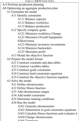
TABLE 1:IDEF0 NODE INDEX.

A-0 Perform production planning

A0 Optimizing an aggregate production plan A1 Formulate the model

A11 Identify constraints A111 Balance capacity A112 Balance workforce A113 Balance production A12 Specify company goals

A121 Minimize workforce Change A122 Maximize Overall Equipment Effectiveness

A123 Minimize inventory investments A124 Minimize backorders

A125 Maximize profit A13 Model the objective function A2 Prepare the model format

A21 Construct constants and data tables A22 Construct variables tables

A23 Construct goals constraints

A24 Construct hard constraints equations A25 Construct the objective function equation A3 Solve the model

A31 Define chromosomes A32 Define fitness function A33 Add chromosomes ranges A34 Add model constraints A35 Determine running conditions A36 Run the model

A361 Generate chromosomes

A362 Substitution in goal constraints equations A363 Calculate fitness functions and evaluates it A364 Change chromosomes

A365 Terminate

IV. APPMODEL SYSTEM ANALYSIS

The A-0 diagram shown in Fig. 3 is the top-level context diagram, on which the subject of the model is represented by a single box with its bounding arrows.

This diagram, which is “perform production planning”, represents the basic and main function of the model, which is to optimize an aggregate production plan.

Fig. 3: Node A-0; perform production planning.

labor hours needed. The mechanism used is the goal programming formulation with the genetic algorithm as a solution methodology.

The A-0 diagram is decomposed to the next level diagram; the A0 diagram shown in Fig. 4, which is decomposed into three functions. These functions are the main activities in optimizing an aggregate production plan using the proposed model.

Fig. 4: Node A0; optimizing an aggregate production plan.

The first activity is the formulation of the model using the goal programming technique. This activity uses the planning parameters and company objectives data as inputs, and results in the mathematical formulation and the hard constraints affecting the other two activities.

The second activity is translating the mathematical model into a computer recognizable format, which is represented by excel spreadsheets. The cells in the spreadsheets represent the objective function, the decision variables, and the deviational variables of the model.

The third activity is the solution of the model. The tool used is the GeneHunter by Ward Systems, which is an excel add-in. GA is used to solve the APP model formulated by activity A1 and formatted by activity A2 and results in a near optimum production plan.

A. Formulate the Model – Node A1

The decomposition of node A1 is shown in Fig. 5, which clarifies the details of the model formulation activity. The model formulation is done by three main activities: identify constraints, specify company goals, and finally model the objective function.

Fig. 5: Node A1; formulate the model.

Identifying constraints yields the hard constraints equations, which act as the control on the company objectives and goals. Identifying the company goals yields the goal constraint equations, which beside the hard constraints; act as the controls on the main objective function.

The goal programming formulation is quite different from other formulation and this is because the objectives are dealt with as constraints. To transform these objectives into constraint equations there must be a target level, which is the aspiration level. Accordingly, the summation of an objective and the deviations set for that objectives are equal to the aspiration level. Consequently, the objective function is to minimize these deviations.

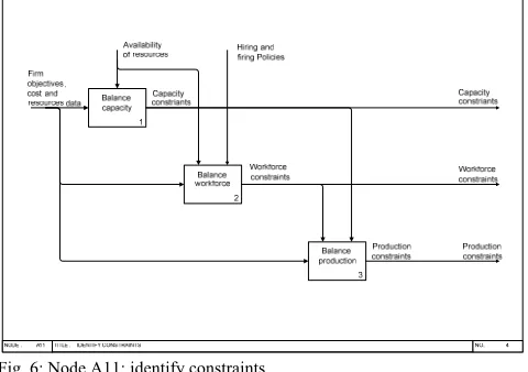
1) Node A11: Identify Constraints

Node A11 is shown in Fig. 6. It explains constraints identification in more detail. The capacity and the workforce serve as a constraint on the production.

The capacity is constrained by the resources available like the number of machines available, normal production time, overtime production time, availability of the machines and system efficiency. The workforce level is also constrained by the resources availability and the hiring and firing policies of the country and the company. The production activity tries to satisfy the company objectives while meeting the capacity and workforce constraints.

The output of the formulation process is the capacity constraint equations, workforce constraint equations, and production constraint equations. These constraints form the hard constraints of the problem that control the process of specifying company goals.

Fig. 6: Node A11; identify constraints.

2) Node A12: Specify Goals

The goals of a company that are defined by the decision makers are presented by node A12 (Fig. 7). Five main goals are defined in the model; maximize profit, minimize backorder, minimize inventory, maximize OEE, and minimize workforce change. The interaction between these goals are clearly identified in this node.

contradicts with the objective of inventory minimization. In addition, minimizing inventory and minimizing backorders are also constrained by each other. Increasing inventory prevents backorders and minimizing inventory can permit backorders.

Fig. 7: Node A12; specify company goals.

B. Prepare the Model Format – Node A2

Node A2 clarifies how the mathematical formulation of the APP model is transformed into excel format. Fig. 8 shows the five main steps to prepare the model format.

TITLE:

NODE : A2 PREPARE THE MODEL FORMAT NO .: 6

1 Construct constants and

data tables

2 Construct variables tables

3 Construct

goals constraints

equations

5 Construct the

objective function equation Hard and

goal constraints Mathematical formulation

Planning parameters and constants

Constants and data tables

Decisions variables

Deviational variables

Decisions variables

Deviational variables

Objective function

Excel

4 Construct hard constraints equations

Fig. 8: Node A2; prepare the model format.

1) Node A21: Construct Constants and Data Tables

The entire company data, planning parameters and constants, and the various costs are organized into excel tables, like number of periods, capacity in each period, machine time to produce one unit, labor time per unit… etc. Fig. 9 shows a sample of these data in excel tables.

Fig. 9: Some of model constants and parameters in excel.

2) Node A22: Construct Variables Tables

The variables are divided into two main sections. Section one contains the variables of each period like hiring and firing in each period, and labor level in each period. Section two contains the variables of each product in each period like the production units, the overtime units, the subcontracting units, the sales units, and the inventory units. Each section is organized into separate tables.

3) Node A23: Construct Goals Constraints Equations

Because the model is formulated as a goal-programming model, the objective functions are transformed into goal constraints. The main objective function is to minimize the deviations from the goal levels. In these goal constraint equations, there are variables that change from iteration to another. Each time the value of these variables change, the deviations are calculated.

4) Node A24: Construct Hard Constraints Equations

The hard constraints are divided into three main groups. Group one is constraints that contain equality sign. These constraints are programmed in excel. Equation cells can use any of excel function to calculate the value of these equations. In this way, the equality constraints can be easily satisfied in the excel environment.

Group two are constraints that contain greater than or smaller than signs (inequality) like constraints. These constraints must be prepared into excel cells before being used by the genetic algorithm tool. These constraints are hard constraints taken from the mathematical model and organized in excel using all the parameters and constants needed from the organized tables as mentioned before.

Group three are constraints that consist of two variables multiplied by each other and equal to zero. Therefore, only one of these variables can have a value and the other will be equal to zero. For example, no inventory and backorder can occur in the same time.

5) Node A25: Construct the Objective Function

The objective function must be prepared into excel cells. As mentioned before, the objective function is to minimize the deviations of the goals, this means minimizing the underachievement or overachievement of each goal, depending on the goal. The deviation cells equal to the aspiration level minus the objective function. The aspiration level is constant and defined by the company, but the objective function changes from one iteration to another. In genetic algorithm, iterations are called generations. Thus, from generation to generation, the objective functions change and consequently, the deviations are recalculated.

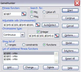
C. Solve the Model – Node A3

As clearly indicated in Fig. 10 (GeneHunter main interface), there are a number of parameters that need to be defined prior to running the model and obtaining the results. Node A3 (Fig. 11) explains how these parameters are defined and how the model is solved using GeneHunter.

Fig. 11: Node A3; solve the model.

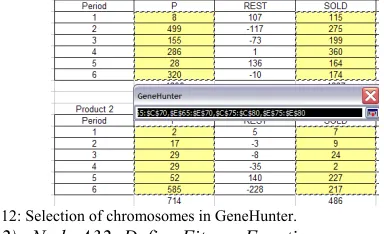
1) Node A31: Define Chromosomes

The chromosomes are the decisions variables and must be specified at first. The user chooses the chromosome from the GeneHunter box as depicted in Fig. 12. The chromosomes in the present model have been chosen to be production units of each product in each period, sales of each product in each period, and the workforce level in each period.

Fig. 12: Selection of chromosomes in GeneHunter.

2) Node A32: Define Fitness Function

The fitness function in the genetic algorithm is equivalent to the objective function in the mathematical modeling. In GeneHunter, the user can specify more than one fitness function, which is a good advantage, because multiple objectives can be dealt with at the same time, instead of satisfying one single objective.

3) Node A33: Add Chromosome Ranges

After defining the chromosomes, the chromosome ranges must be added. These ranges represent the upper and lower bounds of each chromosome. The GeneHunter assures that these ranges are satisfied and, hence, they are called hard constraints. These ranges come from the hard constraint equations in the mathematical formulation.

4) Node A34: Add Model Constraints

The constraints added here in GeneHunter are those of Group two where the constraints are inequality equations, as shown in Fig. 13. The constraints of the first and third groups are satisfied directly in Excel (refer to Node A24).

Fig. 13: Adding constraints in GeneHunter.

GeneHunter considers these constraints as soft constraints; where in each solution, some of these constraints can be

satisfied, and others can be violated. However, based on the mathematical formulation, these constraints must not be violated.

This problem is overcome by using the “IF” function of Excel, where an “IF” function is defined in a cell beside each constraint. If the constraint is satisfied, the cell is equal to zero; if it is not satisfied; the cell is equal to one indicating a penalty factor to be applied to the fitness function. Consequently, GeneHunter tries to minimize the number of unsatisfied constraints to overcome the penalties applied.

5) Node A35: Determine Running Conditions

Before running the GeneHunter, a number of running conditions must be specified. These are typically population size, chromosome length, and evolution parameters such as crossover rate, mutation rate, generation gap, elitism, and diversity. In addition to other optional settings like showing graphs, screen updates, random seed…etc. These settings affect the quality of the solution from the optimality point of view. Furthermore, the settings can adversely affect the time needed to execute a run.

1) The Population Size: the size of the pool, within which the genetic algorithms search for the solution. The size means the number of individuals. Normally increasing the population size means increasing the search time and vice versa. On the other hand, decreasing the population size too much means that there will be a little difference between the individuals which affects the quality of the solution.

2) The Chromosome Length: the number of genes in a chromosome. There are three options 8-bits, 16-bits, or 32-bits. Increasing the number of genes means increasing the precision of the variables, and increasing the time needed to reach good solutions.

3) Crossover Rate: the probability that crossover is applied to chromosomes during generations. The rate can take any value from 0 to 1 and should be set high because it diverse the population. Hence, new generations are produced with many new off springs and some few old parents, which give better solutions.

4) Mutation Rate: the probability that the mutation will be applied to chromosomes during generations. The probability can take a value from 0 to 1 and should take a low value. Mutation prevents the solution to be trapped in local minimum or local maximum. If mutation rate is set to a high value, this will prevent the model from reaching a good solution because good solutions may be changed with mutation process.

5) Generation Gap: the percentage of individuals from the population that will not live in the next generation. This number tends to be high. The remainder of the generation gap represents the percentage of individuals that will be transferred to the next generation.

6) Elitism: this can be set on or off. If it is on, the individuals who will travel to the next generation are the elitist ones, but if it is off then the individuals who will travel to the next generations are chosen randomly. It is better to turn it on.

as opposite to the major changes in individuals that the mutation operator can produce.

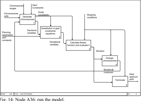
6) Node A36: Run the Model

Node A36 has been decomposed further, as shown in Fig. 14, to explain in more details the model running steps.

TITLE:

NODE : A36 RUN THE MODEL NO .: 8

1 Generate chromosomes

2 Substitution in goal constraints

equations.

3 Calculate fitness function and evaluate it

4 Change chromosomes

5 Terminate Chromosomes

cells Chromosomes ranges

Hard Constraints

Goals constraints

Planning parameters and constants

Decisions variables

Deviational variables

Stopping conditions

Decision

Near optimum APP Mutation & crossover

Fig. 14: Node A36; run the model.

a) Node A361: Chromosomes Generations

First, a number of chromosomes are generated, which represent the individuals of the population. The population size is predetermined in the running conditions. These chromosome must be within ranges and do not violate the hard constraints. However, the solution starts with some chromosomes that are out of range or do not satisfy the constraints. After a few number of generations, the chromosomes generated will be in range and adhere to the specified constraints.

b) Node A362: Equations Substitutions

The chromosomes in the model represent the decision variables. After these chromosomes are generated, their values are then substituted in the goal constraint equations. Each goal constraint equation at this stage contains one unknown variable, which is the deviational variable. The deviational variable for each goal constraint equation is calculated. These deviational variables represent the fitness function, which need to be minimized.

c) Node A363: Fitness Function Calculation

In each generation, the fitness functions are calculated for each individual and the individuals are ordered according to the fittest one. If the elitism operator is on, then the fittest individual will travel to the next generation. If it is off, random individuals will travel to the next generation. The best-fitted individuals and the best fitness functions are displayed on screen.

d) Node A364: Chromosomes Changes

After the fitness functions are calculated and ordered according to the fittest individuals in a generation, the GeneHunter creates another generation by crossover and mutation of some of the chromosomes in the previous generation. The GeneHunter continues producing different generations until a termination criterion is satisfied.

e) Node A365: Termination Criteria

In the GeneHunter tool, three termination criteria can be chosen together or separately.

1) The first is time, where GeneHunter stops at a certain run time preset by the user.

2) The second is number of generations, where GeneHunter stops after reaching a predetermined number of generations.

3) The third one is the number of generations where the fitness functions did not change and this is the best one and the most recommended.

These three criteria have been tested in the model, and it has been shown that using the third one separately is the best choice and results in a near optimum aggregate production plan.

V. CONCLUSION

This paper presented the use of a structured systems analysis methodology to help in the development of a multi-objective aggregate production planning model using a genetic algorithm approach. The methodology chosen is the integrated definition for function modeling level 0 (IDEF0).

The use of the IDEF0 is very useful in the model development stage. It helps the model developer to clarify the model inter-relationships and model logic and to whatever level of detail needed, which is a great help for enhancing the model development process both from the level of understanding and from the development time points of view.

The APP model development process has been described in details using the IDEF0 and has shown its potential role in improving this process.

REFERENCES

[1] E. Khmelnitsky and K. Kogan, "Optimal policies for aggregate production and capacity planning under rapidly changing demand

conditions.," International Journal of Production Research, vol. 34, pp.

1929-1941, 1996.

[2] H. Hwang and C. N. Cha, "An improved version of the production switching heuristic for the aggregate production planning problem,"

International Journal of Production Research, vol. 33, pp. 2567-2577,

1995.

[3] M. N. Fors, K. S. El-Kilany, and M. M. Ghazy, "multi-objective aggregate production planning problem by genetic algorithm approach," presented at 37th Computers and Industrial Engineering Alexandria, Egypt, 2007.

[4] A. M. Masud and C. I. Hwang, "An aggregate production planning model and application of three multiple objective decisions methods.,"

International Journal of Production Research, vol. 18, pp. 741-752,

1980.

[5] S. Kappes, "Putting your IDEF0 model to work," Business Process

Management Journal, vol. 3, pp. 151-161, 1997.

[6] A. Plaia and A. Carrie, "Application and assessment of IDEF3 - process

flow description capture method," International Journal of Operations

& Production Management, vol. 15, pp. 63-73, 1995.

[7] J. Fülscher and S. G. Powell, "Anatomy of A Process Mapping

Workshop," Business Process Management Journal, vol. 5, pp.

208-237, 1999.

[8] "INTEGRATION DEFINITION FOR FUNCTION MODELING (IDEF0)," vol. 2003: National Institute of Standards and Technology, 1993.

[9] T. Perera and K. Liyanage, "IDEF based methodology for rapid data

collection," Integrated Manufacturing Systems, vol. 12, pp. 187-194,

2001.