Assembling homology classes in automorphism groups of free groups

warwick.ac.uk/lib-publications

Original citation:

Conant, James, Hatcher, Allen, Kassabov, Martin and Vogtmann, Karen. (2016) Assembling homology classes in automorphism groups of free groups. Commentarii Mathematici Helvetici .

Permanent WRAP URL:

http://wrap.warwick.ac.uk/80435

Copyright and reuse:

The Warwick Research Archive Portal (WRAP) makes this work by researchers of the University of Warwick available open access under the following conditions. Copyright © and all moral rights to the version of the paper presented here belong to the individual author(s) and/or other copyright owners. To the extent reasonable and practicable the material made available in WRAP has been checked for eligibility before being made available.

Copies of full items can be used for personal research or study, educational, or not-for-profit purposes without prior permission or charge. Provided that the authors, title and full

bibliographic details are credited, a hyperlink and/or URL is given for the original metadata page and the content is not changed in any way.

Publisher’s statement:

To appear in Commentarii Mathematici Helvetici: http://www.ems-ph.org/journals/journal.php?jrn=cmh

A note on versions:

The version presented here may differ from the published version or, version of record, if you wish to cite this item you are advised to consult the publisher’s version. Please see the ‘permanent WRAP URL’ above for details on accessing the published version and note that access may require a subscription.

ASSEMBLING HOMOLOGY CLASSES IN AUTOMORPHISM GROUPS OF FREE GROUPS

JAMES CONANT, ALLEN HATCHER, MARTIN KASSABOV, AND KAREN VOGTMANN

Abstract. The observation that a graph of rankncan be assembled from graphs of smaller rank

k withs leaves by pairing the leaves together leads to a process for assembling homology classes for Out(Fn) and Aut(Fn) from classes for groups Γk,s, where the Γk,sgeneralize Out(Fk) = Γk,0

and Aut(Fk) = Γk,1. The symmetric group Ss acts on H∗(Γk,s) by permuting leaves, and for

trivial rational coefficients we compute theSs-module structure on H∗(Γk,s) completely for k≤

2. Assembling these classes then produces all the known nontrivial rational homology classes for Aut(Fn) and Out(Fn) with the possible exception of classes forn = 7 recently discovered by L.

Bartholdi. It also produces an enormous number of candidates for other nontrivial classes, some old and some new, but we limit the number of these which can be nontrivial using the representation theory of symmetric groups. We gain new insight into some of the most promising candidates by finding small subgroups of Aut(Fn) and Out(Fn) which support them and by finding geometric

representations for the candidate classes as maps of closed manifolds into the moduli space of graphs. Finally, our results have implications for the homology of the Lie algebra of symplectic derivations.

Introduction

In this paper we develop a new approach to studying the homology of automorphism groups of free groups which gives fresh group theoretic and geometric insight into known families of homology classes, and also helps direct the search for new classes. We restrict attention to homology and

cohomology with untwisted coefficients in a field kof characteristic zero unless explicitly specified

otherwise.

Let us recall briefly what is known about these homology groups. First of all, Hi Aut(Fn) and

Hi Out(Fn) are finite-dimensional over k for all i, and vanish for i greater than the virtual

cohomological dimension (vcd), which is 2n−2 for Aut(Fn) and 2n−3 for Out(Fn) [14]. The

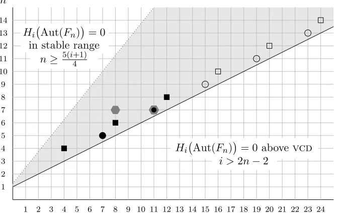
groupsHi Aut(Fn)andHi Out(Fn)are independent ofnforn≥5(i+ 1)/4 as shown in [23, 24],

and these stable groups are in fact zero as well, as Galatius proved in [16]. Thus in the first quadrant

of the (i, n) plane (see Figure 1 below) there is a wedge-shaped region bounded by lines of slope 1/2

and 5/4 that contains all the nonzero groups Hi Aut(Fn)

, and similarly forHi Out(Fn)

. There

are only a small number of these groups which are explicitly known to be nonzero. For Aut(Fn) these

occur for (i, n) = (4,4), (7,5), (8,6), (8,7),(11,7) and (12,8); for Out(Fn) the list is the same except

that (7,5) is omitted. (The natural map Hi Aut(Fn)

→ Hi Out(Fn)

is known to be surjective

for all i and n [27] and we give a different proof of this in Theorem 1.4.) These low-dimensional

calculations are done mostly by computer; see [23, 33, 12, 17, 19, 1]. Complete calculations of

Hi Aut(Fn) have been made only for n≤5 and for Hi Out(Fn) only for n≤7.

There are two potentially infinite sequences which begin with nontrivial classes: these are classes

µk for (i, n) = (4k,2k+ 2) defined by Morita [33] and classes Ek for (i, n) = (4k+ 3,2k+ 3)

constructed in [10]. The latter are known as Eisenstein classes because they arise from Eisenstein

series via the connection between modular forms and the cohomology of SL2(Z) established by the

i n

1 2 3 4 5 6 7 8 9 10 11 12 13 14 15 16 17 18 19 20 21 22 23 24 1

2 3 4 5 6 7 8 9 10 11 12 13 14

Hi Aut(Fn)= 0 abovevcd

i >2n−2

Hi Aut(Fn)= 0 in stable range

n≥ 5(i₄+1)

Figure 1. Classes in the homology ofAut(Fn) forn≤24. The Morita classes are

shown as squares and the Eisenstein classes are shown as circles, filled in if the classes are known to be nontrivial. The nontrivial classes recently found by Bartholdi are shown as hexagons.

Eichler-Shimura isomorphism. The Morita classes µk are defined for both Aut and Out, while the

E_k’s are defined for Aut and map to zero in Out. Note that these classes are all either one or two

dimensions below thevcd.

One of the big open questions is to determine which of the classesµkandEkare nonzero. However,

even if they are nonzero it seems that they account for only a small fraction of the homology. The

Euler characteristic for H∗ Out(Fn)

was computed for n ≤ 11 by Morita, Sakasai, and Suzuki

in [35, 36], and after starting with the values 1 and 2 for n≤8, it becomes −21,−124,−1202 for

n = 9,10,11. If this trend continues for larger n, it would say there are many odd-dimensional

classes for Out(Fn), though the only one discovered to date is the 11-dimensional class in Out(F7)

recently found by Bartholdi [1]. (This class is balanced by a single 8-dimensional class, consistent

with the Euler characteristic calculation for n= 8.)

n 3 4 5 6 7 8 9 10 11 12

χ(Out(Fn)) 1 2 1 2 1 1 −21 −124 −1202 ?

Figure 2. Euler characteristic ofOut(Fn)

The Morita classes µk were first constructed using Lie algebra techniques underpinned by

Kontse-vich’s “formal noncommutative symplectic geometry” [28, 29]. In [12] these classes were interpreted

explicitly in Lie graph cohomology and generalized; further generalizations including the classesEk

were obtained using “hairy graph homology” in [10]. In the present paper we show how to construct all of these classes in an elementary fashion which bypasses both graph homology and Kontsevich’s

work. The idea is to use the fact that Out(Fn) and Aut(Fn) are the first two groups in a series

Γn,0,Γn,1,Γn,2,· · · where Γn,s is the group of homotopy classes of self-homotopy equivalences of a

rankngraph fixingsleaves (vertices of valence one) [2, 22, 24]. These groups are related by natural

surjective homomorphisms Γn,s→Γn,s−k with kernel (Fn)k. These homomorphisms split fork < s

but not fork=s.

The groups Γn,sare of interest because by gluing graphs together along a subset of their leaf vertices

we obtain many homomorphisms Γn1,s1 × · · · ×Γnk,sk →Γn,s. On the level of homology, each such

map induces a homomorphism

H∗(Γn1,s1)⊗ · · · ⊗H∗(Γnk,sk)−→H∗(Γn,s),

which we call anassembly map (see Section 4). For example by pairing up all of the leaves of two

rank one graphs with sleaves (in any way) we obtain an assembly map

H∗(Γ1,s)⊗H∗(Γ1,s)−→H∗(Γ2s+1,0) =H∗ Out(F2s+1)

.

Restricting to the case thatsis odd, says= 2k+1, it is easy to calculate thatH2k(Γ1,2k+1)∼=k(see

Section 2.4), and in Section 4.1 we note that the Morita classµk is the image ofαk⊗αk under this

assembly map, whereαkis a generator ofH2k(Γ1,2k+1). This graphical interpretation of the original

Morita series allows us to give two new proofs that Morita classes vanish after one stabilization, one proof being algebraic (Section 5.2) and the other geometric (Section 6). This result was first proved via a more elaborate combinatorial computation in graph homology in [13].

As a consequence of the elementary construction, we find that all the classesµk in Morita’s original

series, as well as the generalized Morita classes given in [12], are supported on abelian subgroups

of Aut(Fn). This naturally gives rise to the question of whether the standard maximal abelian

subgroup can support nontrivial homology classes, and we show in Section 7 that it cannot. For the Eisenstein classes we find slightly more complicated nonabelian subgroups that support them.

Parallel to these group-theoretic descriptions of Morita and Eisenstein classes there are geometric

representations as maps of closed orientable manifolds into the classifying spaces for Aut(Fn) or

Out(Fn) carrying top-dimensional homology classes of the manifolds to the Morita or Eisenstein

classes. In the case of Morita classes the manifolds are tori while for the Eisenstein classes they are products of a certain 3-manifold with tori.

The computational heart of the paper is in Section 2 where we use the natural action of the

symmetric group Ss on Γn,s to study H∗(Γn,s). Forn= 1 andn= 2 we determine theSs-module

structure ofH∗(Γn,s) completely. This can be applied in the search for nontrivial classes inH∗(Γn,s)

that lie in the images of assembly maps. In particular we show in Section 4.5 that many of the

generalized Morita classes are in fact zero, though this does not apply to the µk’s themselves. In

Section 4.7 we show that certain odd-dimensional classes constructed in [35] must vanish, but we also find some new candidates for nontrivial odd-dimensional classes.

The calculation ofH∗(Γ1,s) is an easy consequence of the fact that Γ1,s ∼=Z2n Zs−1. To calculate

the homology of Γ2,s we use the short exact sequence

1−→F₂s−→Γ2,s −→Γ2,0= Out(F2)−→1.

In the Leray-Serre spectral sequence associated to this short exact sequence we note that all dif-ferentials are zero, allowing us to completely calculate the homology. (Actually, for convenience we use cohomology rather than homology for spectral sequence arguments and indeed for most

algebraic calculations.) The results of our computations for n= 1 and n= 2 and small values ofs

are recorded in several tables at the end of the paper.

These computations show that even though the dimension of Hi(Γn,s) as a vector space over k

increases withsfor fixedn= 1,2, it is nevertheless true that as representations ofSs these vector

spaces eventually stabilize in the sense of [7]. This representation stability holds for all n in fact,

as a corollary of a result of Jim´enez Rolland [26]; see Proposition 5.1.

We also apply some elementary representation theory to show that the groupHi(Γn,s) is nontrivial

whenever i is an even multiple of n and s is sufficiently large with respect to i and n. This can

be contrasted with the situation for stabilization with respect ton, whereHi(Γn,s) becomes trivial

as n increases, by Galatius’ theorem for s = 1 and hence for all s since the groups Hi(Γn,s) are

independent of bothnand swhen n≥2i+ 4 by [24].

In Section 8 we point out the relationship of the homology of Γn,s with both hairy graph

ho-mology [10, 11] and the cohoho-mology of the Lie algebra of symplectic derivations, as studied by

Kontsevich, Morita and many others. In particular, we show how our computations for Γn,s

im-ply that the cohomology in each dimension of this Lie algebra contains infinitely many simple Sp-modules.

Section 9 contains some conjectures and open questions. Most nontrivial rational homology classes

for any Γn,s which occur below thevcd2n−3 +shave been shown to be in the image of assembly

maps. The only exceptions are new classes for Out(F7) and Aut(F7) recently found by Bartholdi [1],

for which this is still unclear. It is then natural to ask whether assembly maps generate all classes

below thevcd. The number of potential homology classes forHi(Γn,s) constructed from assembly

maps grows exponentially with n, leading to the expectation that the rank of the homology also

grows very fast. Fors= 0 this expectation coincides nicely with the Euler characteristic calculations

of Morita, Sakasai, and Suzuki cited earlier.

Finally, we remark that the rational classifying spaces for the groups Γn,s have natural

compactifi-cations, whose homology has recently been studied by Chan, Galatius and Payne ([5, 6]). One thing

they show is that this homology vanishes in dimensions less than s−3. It is easy to see that all

homology classes which are in the image of an assembly map must vanish in this compactification, consistent with their calculations.

Acknowledgements: Martin Kassabov was partially supported by Simons Foundation grant 305181 and NSF grants DMS 0900932 and 1303117. Karen Vogtmann was partially supported by NSF grant DMS 1011857 and a Royal Society Wolfson Award.

1. The groups Γn,s

1.1. Definitions. The group Out(Fn) is the group of homotopy classes of self-homotopy

equiva-lences of a finite connected graphX of rankn, and Aut(Fn) is the basepointed version of this, the

homotopy classes of homotopy equivalences of X fixing a basepoint, where homotopies are also

re-quired to fix the basepoint. A natural generalization is to choosesdistinct marked pointsx1, . . . , xs

inX and then define Γn,s to be the group of homotopy classes of self-homotopy equivalences ofX

fixing each xi, with homotopies also required to fix these points. The group operation in Γn,s is

induced by composition of homotopy equivalences, which is obviously associative with an identity element. To check that inverses exist one uses the following elementary fact:

Lemma 1.1. If f : X → Y is a homotopy equivalence of finite connected graphs taking a set of s marked points x = {x1, . . . , xs} bijectively to another such set y = {y1, . . . , ys}, then f is a homotopy equivalence of pairs (X,x)→(Y,y), so there is a map g:Y →X restricting to f−1 on y with the compositions gf and f g homotopic to the identity fixing x and y respectively.

Proof. LetZbe the quotient of the mapping cylinder offobtained by collapsingx×Itox=y. The

quotient map collapses a finite number of intervals to a point so it is a homotopy equivalence. Iff

is a homotopy equivalence, then the inclusions ofX andY into the mapping cylinder are homotopy

equivalences, hence the same is true for the inclusions intoZ. It follows thatZ deformation retracts

onto the copies of X and Y at either end. The deformation retraction toX gives the map g.

This lemma also shows that Γn,s does not depend on the choice of (X,x), up to isomorphism.

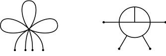
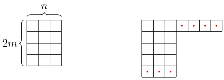
Throughout most of the paper we will take X to be a rank n graph with exactly s leaves, with

the leaf vertices as the marked points. Here a leaf means a vertex of valence one together with

the adjoining edge. Our generic notation for a graph of rank n with s leaves will be Xn,s. Two

examples of rank 3 graphs with 4 leaves are shown in Figure 3.

Figure 3. Two possibilities for X3,4

A homotopy equivalencef :Xn,s →Xn,s that permutes the leaf vertices induces an automorphism

of Γn,svia conjugation byf. Iff fixes the leaf vertices this is an inner automorphism, hence induces

the identity on the homology of Γn,s, so there is an induced action of the symmetric group Ss on

the homology. If we chooseXn,s to have a single nonleaf vertex as in the left half of Figure 3 then

this action ofSson homology comes from the action on Xn,s permuting the leaves. TheSs-action

on H∗(Γn,s) will play a major role in later sections of the paper.

The groups Γ0,s are trivial since anyX0,s is a tree and any homotopy equivalence of a tree which

fixes all of its leaf vertices is homotopic to the identity by a homotopy fixing the leaf vertices.

As shown in [2], the group Γ1,s is the semidirect product Z2 n Zs−1. The free abelian subgroup

Zs−1 is generated by homotopy equivalences which wrap one leaf edge around the (unique) loop

while fixing the leaf vertex and the rest of the graph. These generators commute since they have disjoint supports. Note that wrapping all of the leaf edges around the loop in the same direction

results in a map which is homotopic to the identity fixing the leaf vertices, so there are onlys−1

independent generators. The generator ofZ2 flips the loop, so acts on Zs−1 by x7→ −x.

We remark that Γn,scould also be defined as the mapping class group of the 3-manifoldMn,sformed

by removing sdisjoint balls from the connected sum of ncopies ofS1_×S2_{, modulo the subgroup}

generated by Dehn twists along embedded 2-spheres. This follows from results of Laudenbach and is made explicit in Proposition 1 of [24].

The groups Γn,s for s > 1 were first considered in [22] in work on homological stability and also

appeared in Bestvina and Feighn’s proof that Out(Fn) is a virtual duality group [2]. It was observed

in [10] that their homology is very closely related to hairy graph homology groups for the Lie operad.

1.2. Short exact sequences. In this section we observe that there are natural short exact

se-quences relating the groups Γn,s.

Proposition 1.2. If n >1 and k≤sthere is a short exact sequence

1−→F_nk−→Γn,s−→Γn,s−k−→1

which splits if k < s. This holds also when n= 1 and k < s, but in the exceptional case (n, k) = (1, s) there is a split short exact sequence

1−→Zs−1 −→Γ1,s −→Γ1,0 −→1

expressing Γ1,s as the semidirect productZ2n Zs−1.

Fork=s−1 the proposition follows from [2], section 2.5, where it is shown that Γn,s∼= Aut(Fn)n

F_ns−1.

Proof. LetX be a rankngraph containing a setx={x1, . . . , xs}of sdistinct marked points. Let

En,s be the space of homotopy equivalences X → X fixed on x, so Γn,s = π0(En,s). For k ≤ s

there is an inclusion En,s ⊂ En,s−k obtained by no longer requiring homotopy equivalences to fix

x1, . . . , xk. Evaluating homotopy equivalences X → X on x1, . . . , xk gives a map En,s−k → Xk

which is a fibration with fiberEn,sover the point (x1, . . . , xk). The long exact sequence of homotopy

groups for this fibration ends with the terms

π1(En,s−k)−→π1(Xk)−→Γn,s −→Γn,s−k−→1.

Whenk < sthe first termπ1(En,s−k) is trivial by obstruction theory. Namely, we can assumeX is

obtained by attaching 1-cells to a set of s−k0-cells, and then any loop of homotopy equivalences

ft:X→X fixing the 0-cells can be deformed to the trivial loop sinceπ2(X) = 0. Thus we obtain

the first short exact sequence in statement of the proposition when k < s, for arbitrary n.

To split this short exact sequence whenk < sit suffices to find a mapEn,s−k→En,s such that the

compositionEn,s−k→En,s →En,s−kis homotopic to the identity. We are free to choose the marked

pointsx1, . . . , xk anywhere in the complement of the remainings−kpoints, so we choose them in

a small contractible neighborhood N of the point xk+1. We can then deformation retract En,s−k

onto the subspaceE_n,s0 _−k of homotopy equivalences that are fixed onN. (This is particularly easy

if we chooseXto have a valence one vertex withxk+1as this vertex.) The subspaceEn,s0 −kincludes

naturally intoEn,s, and this inclusion gives the desired map En,s−k →En,s as the composition of

the first two mapsEn,s−k→E_n,s0 −k,→En,s,→En,s−k, the first map being the retraction produced

by the deformation retraction. The composition of the three maps is homotopic to the identity by the deformation retraction itself.

There remain the cases k = s. The issue is whether π1(En,0) is trivial, so that the long exact

sequence becomes a short exact sequence. To settle this, consider the fibration En,1 →En,0 →X

which gives a long exact sequence

1−→π1(En,0)−→π1(X)−→Γn,1 −→Γn,0 −→1

where the initial 1 isπ1(En,1). The middle map in this sequence is the map fromπ1 of the base of

the fibration to π0 of the fiber, and it is easy to check the definitions to see that this is the map

Fn→ Aut(Fn) sending an element of Fn to the inner automorphism it determines. The kernel of

this map is the center of Fn so it is trivial whenn >1 and we deduce that π1(En,0) = 1 in these

cases, so we again have the short exact sequence claimed in the proposition.

When n= 1 and k=sthe space E1,0 is homotopy equivalent to S1 and the exact sequence of the

fibrationE1,s →E1,0 →Xs becomes

1−→_Z−→_Zs−→Γ1,s −→Γ1,0 −→1,

with the mapZ→Zs the diagonal inclusion. This yields the short exact sequence displaying Γ1,s

as the semidirect productZ2n Zs−1.

Remark 1.3. If we use Laudenbach’s theorem to express Γn,s in terms of the mapping class group of

Mn,s then the short exact sequence of Proposition 1.2 can be derived from a 3-dimensional analog

of the Birman exact sequence for mapping class groups of surfaces [2]. From this viewpoint the

space En,s is replaced by the diffeomorphism group of Mn,s, and the resulting fibration is a very

simple special case of much more general fibrations due to Cerf, Palais, and Lima.

1.3. Homology splitting. Ifs=k and n≥2 the map Γn,s →Γn,s−k = Γn,0 does not split. The

reason is that Γn,0 = Out(Fn) contains finite subgroups which do not lift. For example, consider the

symmetry group of the graph consisting of two vertices joined byn+ 1 edges. This is a subgroup of

Γn,0 which cannot be realized on any graph of rankn by graph symmetries which fix a basepoint,

so the subgroup does not lift to any Γn,s withs≥1.

Homology with coefficients inkdoes not see finite subgroups, and in fact when we pass to homology

we do obtain a splitting. Note that it suffices to prove this for s= 1, i.e. the map from Aut(Fn) to

Out(Fn). Homology splitting of this map was first proved by Kawazumi in [27]. There is a simple

proof of this using the fact that the moduli space of graphs (respectively basepointed graphs) is a

rationalK(π,1) for Out(Fn) (respectively Aut(Fn)). The idea is that although there is no natural

way to choose a basepoint in a graph one can compensate by taking a suitably weighted sum of all possible basepoints.

Theorem 1.4. The natural mapAut(Fn)→Out(Fn) splits on the level of rational homology, i.e., Hk Out(Fn)

embeds into Hk Aut(Fn)

.

Proof. We define a backwards map on the chain level. We take C∗ Aut(Fn)

and C∗ Out(Fn)

to be defined in terms of the spine of the moduli space of (basepointed) graphs. We refer to [13,

section 2] for complete details. The chain complexC∗ Aut(Fn)

is spanned by graphs with specified

subforests and a chosen basepoint, whileC∗ Out(Fn)

is defined in the same way except the graphs do not have basepoints. In both cases, the edges in the subforests are ordered, and changing the

order incurs the sign of the permutation. There are two boundary operators∂C and∂Rwhich sum

over contracting and removing forest edges respectively. In both the basepointed and unbasepointed

cases, contracting the ith edge of a forest comes with the sign (−1)i+1, while removing that edge

comes with the sign (−1)i.

The natural projection π: Aut(Fn)→Out(Fn) corresponds to the map

π∗:C∗ Aut(Fn)→C∗ Out(Fn)

which forgets the basepoint.

We now define a map r:C∗ Out(Fn)

→C∗ Aut(Fn)

.by

r(G) = X

v∈V(G)

(|v| −2)rv(G).

Here V(G) is the vertex set of G, |v| is the valence of v and rv(G) is the forested graph G with

v specified as the basepoint. We need to check that r is a chain map. Clearly ∂Rr = r∂R since

the definition of r makes no reference to the forest, and the signs in ∂R make no reference to the

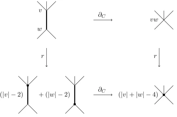
basepoint. For∂C we must check whether the order of performing the two operations of adding a

basepoint and contracting an edge matters, the signs in ∂C being the same in both cases. If e is

an edge with vertices v and w, then adding a basepoint distinct from v and w clearly commutes

with contractinge. Adding basepoints atv and atw followed by contractingeresults in the same

basepointed graph with multiplicity |v|+|w| −4, whereas contracting e first results in a vertex

v

w

∂C

vw

r

(|v| −2) + (|w| −2) ∂C (|v|+|w| −4)

r

Figure 4. Diagram commutes because|vw|=|v|+|w| −2

vw of valence |v|+|w| −2, so adding a basepoint there also gives multiplicity |v|+|w| −4 (see

Figure 4).

Now observe that π∗◦r(G) = kGG, where kG = P_v∈V(G)(|v| −2) = 2n−2. Thus if we are not

in the trivial case n= 1 the composition π∗◦r is represented by a diagonal matrix with nonzero

diagonal entries and is therefore invertible. Sor∗ is injective on homology.

2. Cohomology of Γn,s

We are interested in studying the homology of Out(Fn) and Aut(Fn), with trivial coefficients in

a field k of characteristic 0. The idea is to glue together homology classes of the Γn,s using the

assembly maps described briefly in the Introduction and defined more precisely in Section 4. To find nontrivial classes which can be fed to the assembly maps we use some elementary representation

theory of symmetric groups and GLn(Z) together with the Leray-Serre spectral sequence applied

to the group extensions

(1) 1−→F_ns−→Γn,s−→Γn,0= Out(Fn)−→1

from Section 1.2.

For the calculations it will be convenient to switch from homology to cohomology, which is

iso-morphic by the universal coefficient theorem since we are taking coefficients inkand all homology

is finite-dimensional over k. In the course of our study we will exploit the structure of Hi(Γn,s)

as an Ss-module. Since all the modules we consider are finite-dimensional and all Ss-modules

are self-dual, the cohomology is isomorphic to the homology also as an S_s-module, though the

isomorphism is not canonical.

2.1. A little representation theory. In this section we establish some notation and collect some results from representation theory which we will use. All the contents of this section are well-known and can be found, for example, in [15].

Recall that the irreducible representations of S_s correspond to partitions of s and are often

represented by drawing Young diagrams with s boxes arranged in rows of non-increasing size.

We use Pλ to denote the representation corresponding to the partition λ = (λ1, . . . , λk), where λ1≥λ2 ≥ · · · ≥λk and

P

iλi =s. Exponential notation denotes equal values ofλi, e.g.,P(2,1,1,1,1)

is written as P_(2,14₎.

Example 2.1. The module P_(s) is the1-dimensional trivial module. The moduleP₍₁s₎= alt is the 1-dimensional alternating representation of Ss, where a permutation σ acts as multiplication by

sign(σ) =±1. The module P(s−1,1) is the (s−1)-dimensional standardrepresentation ks/k of Ss.

It contains distinguished elements vi, 1≤i≤s, which satisfy P

vi= 0.

The tensor product of twoS_s-representations is also anS_s-representation with the diagonal action.

In general the multiplicity of an irreducible representation Pν in the decomposition of Pλ⊗Pµ is

difficult to compute, but for ν = (s) it is known that P_(s) occurs with multiplicity 1 if λ=µ and

with multiplicity 0 otherwise. One tensor product we will encounter is Pλ⊗alt. This is equal to

Pλ0 where λ0 denotes the transpose partition, obtained by switching the rows and columns of the

Young diagram.

IfP is a representation of Ss−k andQis a representation of Sk, thenP⊗Qis a representation of

S_s−k×Sk. If we considerSs−k×Sk as a subgroup ofSswe can form the induced representation.

Following Fulton and Harris [15], we denote this induced representation by P◦Q, i.e.,

P ◦Q= IndSs

Ss−k×SkP⊗Q.

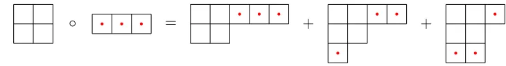
The Littlewood-Richardson rule can be used to compute the decomposition ofPλ◦Pµinto irreducible

modules. When µ= (k) this specializes to thePieri rule, see [15, appendix A]. This says that the

terms of Pλ◦P(k) correspond to all Young diagrams which can be obtained by adding k boxes to

the diagram for λ, each in a different column. An example is illustrated in Figure 5.

Now let V be ann-dimensional vector space. The irreducible representations of GL(V) = GLn(k)

also correspond to partitions, and we let SλV denote the GLn-representation associated to the

partition λ. Since dim(V) = n only partitions into at most n pieces occur. Schur-Weyl duality

gives the irreducible decomposition of the representation V⊗q as a module over GL(V) ×S_q,

namely

V⊗q ∼=M

λ

SλV ⊗Pλ,

where the sum is over all partitions ofq into at mostnpieces (ifλhas more thannrows the module

SλV is zero) (see, e.g., [15], Cor. 6.6). We emphasize that GL(V) acts trivially on Pλ and Sq acts

trivially on SλV.

Example 2.2. For q= 2 the Schur-Weyl formula gives

V ⊗V = S(2)V ⊗P(2)

⊕ S(12₎V ⊗P₍₁2₎

= Sym2V ⊕V2

V.

where Symk denotes thek-th symmetric power functor on vector spaces andVk is the k-th exterior power.

◦ = + +

Figure 5. Pieri rule for decomposingP(2,2)◦P(3)

Notation. We denote by V∧q the Sq-module which is isomorphic as a vector space to V⊗q, with

S_q acting by permuting the factors and multiplying by the sign of the permutation, i.e., V∧q=V⊗q⊗alt.

The Schur-Weyl formula translates to a similar formula for V∧q:

V∧q=V⊗q⊗alt∼=M

λ

SλV ⊗Pλ⊗alt =

M

λ

SλV ⊗Pλ0,

where the sum is over all partitions of q into at mostn pieces.

Finally, we record a computation we will use later.

Lemma 2.3. Suppose dim(V) = 2. ThenS(q−k,k)V = Sym∼ q−2kV ⊗detk asGL(V)-modules, where

detk= (V2

V)⊗k is the 1-dimensional representation given by the k-th power of the determinant.

Proof. This can be seen by calculating the Schur polynomialsSλ for the two sides, which determine

the representations uniquely. Using the formula A.4 of [15, Appendix A] one obtains

S(a,b) = (x1x2)b

hxa−b+1 1 −x

a−b+1 2 x1−x2

i

= (S(1,1))bS(a−b).

The lemma now follows because Schur polynomials of tensor products multiply, S(1,1)H= det and

S(c)V = SymcV.

2.2. The Leray-Serre spectral sequence. Shifting from homology to cohomology now, the

Leray-Serre spectral sequence of a group extension 1 → N → G → Q → 1 is a first-quadrant

spectral sequence with E₂p,q=Hp _Q;Hq_(N)

, which converges to Hp+q_{(G). Applied to the short}

exact sequence (1) it reads

(2) E₂p,q=Hp Out(Fn);Hq(F_ns) =⇒ Hp+q(Γn,s).

The symmetric group Ss which permutes the factors of Fns induces an action on each of the E2

terms which commutes with all differentials. We begin by identifying the coefficients Hq(F_ns) as

S_s-modules.

Throughout this section we set H =H1(Fn) ∼=kn. Note that the action of Out(Fn) on H factors

through the natural GLn(Z) action on H.

Lemma 2.4. The cohomology of F_ns is given as an Ss-module by the formula Hq(F_ns) = H∧q◦P_(s−q).

Proof. The K¨unneth formula gives an isomorphism

H∗(Fn)⊗ · · · ⊗H∗(Fn)∼=H∗(Fn× · · · ×Fn)

via the cohomology cross product. The group S_s acts by permuting the factors, with signs

de-termined by the permutation and the dimension of the cohomology groups on the left-hand side

(see, e.g., [21, Chapter 3B]). The cohomology ofFnisk in dimension 0, H in dimension 1 and zero

in higher dimensions, so in dimension q the cohomology of F_ns is the direct sum of _qs copies of

H⊗q. These copies are permuted by the action of S_s. The stabilizer of each copy is isomorphic

toSq×Ss−q, where the action of Sq on H⊗q is modified by the sign of the permutation since all

classes are in dimension 1.

In other words, Hq(F_ns) is obtained by inducing up to S_s theS_q×S_s−q-module H∧q⊗P(s−q).

We now read off information which we obtain immediately from the spectral sequence (2). The

first observation applies to the cases= 1. The same result was obtained earlier by Kawazumi [27]

using a different method.

Proposition 2.5. There is an isomorphismHkAut(Fn);k∼=HkOut(Fn);k⊕Hk−1 Out(Fn); H.

Proof. In the spectral sequence associated to 1 → Fn → Aut(Fn) → Out(Fn) → 1 we have

E₂p,q ∼= Hp Out(Fn);Hq(Fn) with differentials of bidegree (2,−1). Since Fn has cohomological

dimension one there are only two nontrivial rows, namely q = 0 and q = 1, so the only possible

nonzero differentials in the entire spectral sequence are on the E2 page; they start in the top row

q= 1 with target in the bottom row q = 0.

The map on cohomology induced by p: Aut(Fn) → Out(Fn) factors through the edge

homomor-phisme:E∞p,0→Hp Aut(Fn)

Hp Out(Fn) Hp Aut(Fn)

Hp Out(Fn)/Im(d2)

p∗

e

The top arrow is injective by Theorem 1.4, so the left arrow is as well, i.e., Im(d2) = 0 and the

differentials on theE2 page are also trivial. Thus

Hk Aut(Fn)

=E₂k,0⊕E₂k−1,1

=Hk Out(Fn)

⊕Hk−1 Out(Fn);H1(Fn)

=Hk Out(Fn)

⊕Hk−1 Out(Fn); H

.

The next observation has to do with the top-dimensional cohomology of Γn,s.

Proposition 2.6. Hk_(Γ

n,s)vanishes fork >2n−3+sandH2n−3+s(Γn,s)is given as anSs-module by

H2n−3+s(Γn,s)∼=H2n−3 Out(Fn); H∧s

.

Proof. The cohomology group Hp Out(Fn);Hq(Fns)

vanishes if either p >2n−3 or q > s since

the virtual cohomological dimension of Out(Fn) is 2n−3 and the virtual cohomological dimension

of F_ns is equal to s. Thus the only possible nonzero terms in the spectral sequence (2) lie in a

rectangle withE₂2n−3,s at its upper right-hand corner, so all differentials into or out ofE₂2n−3,s are zero and

H2n−3+s(Γn,s)∼=H2n−3 Out(Fn);Hs(Fns) ∼

=H2n−3 Out(Fn); H∧s

.

2.3. Rank zero. Since Γ0,s is trivial, we just have

Hi(Γ0,s) = (

P_(s) =k ifi= 0

0 ifi6= 0.

2.4. Rank one. For n= 1 the short exact sequence (1) is a restatement of the fact that

Γ1,s =Z2n Zs−1,

where theZ2acts viax7→ −x. We can use this to compute the cohomology of Γ1,s as anSs-module

without appealing to the Leray-Serre spectral sequence, as follows.

Proposition 2.7. As a representation of S_s

Hi(Γ1,s)∼= (

P_(s−i,1i₎ if i is even 0 if i is odd.

In particular, H2k(Γ1,2k+1)∼=P(12k+1₎=k with the alternating action.

Proof. The rational cohomology of Γ1,s = Z2 n Zs−1 is the invariants of the Z2-action on the

cohomology of Zs−1 induced from the action on Zs−1. The cohomology of Zs−1 is the exterior

algebra ons−1 generators. Thus we get the even degree part of this exterior algebra:

Hi(Γ1,s)∼= (_Vi

ks−1 ifiis even

0 ifiis odd.

To see theSs action, write Γ1,s=Z2n(Zs/Z). The representationks/kis the standard

represen-tationP(s−1,1) ofSs, and by [15, Ex. 4.6] we haveVi(ks/k) =P(s−i,1i₎ as an S_s-module.

We record this calculation for small values of sin table form at the end of the paper (Section 10).

We note that the results agree with the calculations via dihedral homology in [11].

2.5. Rank two. Recall that Γ2,0 = Out(F2) ∼= GL2(Z), so that for n = 2 the E2 term of (2)

is

E₂p,q=Hp GL2(Z);Hq(F2s)

.

Since GL2(Z) has virtual cohomological dimension 1, the only potentially nonzero terms on the

E2-page of this spectral sequence lie in the first two columns p = 0 and p = 1. For p = 1 the

cohomology of GL2(Z) is closely related to modular forms; we review this relation in the next

subsection.

2.5.1. Modular forms. LetM_s be the vector space of classical modular forms for SL2(Z) of weight

s, and letSs ⊂ Msbe the subspace of cusp forms. See [31] for an elementary introduction to these

spaces. They satisfy

M

s≥0

M_s∼=k[E4, E6],

whereE4 and E6 are generators of weight 4 and 6 respectively. In particular, Ms is nonzero only

for s >2 even. In these cases the subspace S_s has codimension 1. The classical Eichler-Shimura

isomorphism (see, e.g., [20]) relates modular forms to the cohomology of SL2(Z):

H1 SL2(Z); Syms(k2)∼=Ms+2⊕ Ss+2.

We next review the relation between cusp forms and the stabilizer of the cusp at infinity. Let

P ≤SL2(Z) be the (parabolic) subgroup generated by the matrix (1 10 1) and consider the map

ρ:H1 SL2(Z); Syms(k2)−→H1 P; Syms(k2)

induced by inclusion. SinceP ∼=Z, its first cohomology with any coefficients is simply the

coinvari-ants of the action, which is isomorphic to the space of invaricoinvari-ants. Ifx andy are a basis fork2, the

generator ofP acts on Syms(k2) =k[xs, xs−1y, . . . , xys−1, ys] by sendingx7→x andy7→x+y, so

the space of invariants is 1-dimensional, spanned byxs. The mapρcan be identified with the map

M_s+2⊕ S_s+2→ M_s+2/S_s+2 (which projects onto the first factor and kills the second factor) given

by the normalized value of the modular form at infinity (see [20]).

We can reinterpret ρ in terms of the cohomology of GL2(Z) using the short exact sequence 1 →

SL2(Z)→GL2(Z)→Z2→1 (see, e.g., [10]); this gives

H1 GL2(Z); Syms(k2)⊗det∼=Ms+2 and H1 GL2(Z); Syms(k2)∼=Ss+2.

Since H1 _SL

2(Z); Syms(k2) = Ms+2 ⊕ Ss+2 we see that the restriction of ρ to the second

fac-tor

ρ:H1 GL2(Z); Syms(k2)−→H1 P; Syms(k2)

is zero, but on the first factor

ρ:H1 GL2(Z); Syms(k2)⊗det−→H1 P; Syms(k2)⊗det

has 1-dimensional image when s >0 is even.

2.5.2. Cohomology calculations.

Lemma 2.8. Let H =H1(F2)∼=k2. Then as an Sq-module,

H0 GL2(Z); H∧q= (

P₍₂2m₎ if q= 4m 0 otherwise.

H1 GL2(Z); H∧q=     

   

0 if q is odd

Wq:= M

0≤i<q₂

Xq,i⊗P(2i_,1q−2i₎ if q is even

where X_q,i = S_q+2−2i if i is even and Mq+2−2i if i is odd. In either case Xq,i is trivial as an

Sq-module.

Remark 2.9. The formula in the statement above gives the following pattern for the first few Wq: W0= 0

W2= (S4⊗P(12₎)

W4= (S6⊗P(14₎)⊕(M₄⊗P_(2,12₎)

W6= (S8⊗P(16₎)⊕(M₆⊗P_(2,14₎)⊕(S₄⊗P₍₂2_,12₎)

W8= (S10⊗P(18₎)⊕(M₈⊗P_(2,16₎)⊕(S₆⊗P₍₂2_,14₎)⊕(M₄⊗P₍₂3_,12₎)

W10= (S12⊗P(110₎)⊕(M₁₀⊗P_(2,18₎)⊕(S₈⊗P₍₂2_,16₎)⊕(M₆⊗P₍₂3_,14₎)⊕(S₄⊗P₍₂4_,12₎).

However, the dimension of M_k is 1 for k= 4,6,8,10, and hence the dimension ofS_k is trivial in

those degrees. The module S₁₂ is 1-dimensional, so we see interesting modular forms entering the

picture starting with W10. Using this information, the above list simplifies to

W0 = 0 W2 = 0 W4 =P(2,12₎

W6 =P(2,14₎

W8 =P(2,16₎⊕P₍₂3_,12₎

Proof. We first decompose the coefficients H∧q into irreducible components using Schur-Weyl

dual-ity. Since H has dimension 2, this gives H∧q∼=L_λSλH⊗Pλ0, where the sum is over all partitions

of q into at most 2 pieces, i.e., λ= (q−k, k).

Now H0 _GL

2(Z); H∧q is equal to the GL2(Z)-invariants of H∧q, so we are looking for the trivial

representations SλH appearing in the Schur-Weyl formula. By Lemma 2.3 we have S(q−k,k)H ∼=

Symq−2kH⊗detk, which is clearly trivial only if q= 2kandk is even. Therefore as anSq-module

we have

H0 GL2(Z); H∧q= (

P(2m,2m)0 =P₍₂2m₎ ifq = 4m

0 otherwise.

For the first cohomology we have

H1 GL2(Z); H∧q= M

0≤k≤q₂

H1 GL2(Z);S(q−k,k)H⊗P(q−k,k)0

= M

0≤k≤q₂

H1 GL2(Z);S(q−k,k)H

⊗P(q−k,k)0

= M

0≤k≤q₂

H1 GL2(Z); Symq−2kH⊗detk⊗P(q−k,k)0

= M

0≤k≤q₂

H1 GL2(Z); Symq−2kH⊗detk⊗P(2k_,1q−2k₎.

The computations in Section 2.5.1 now give

H1 GL2(Z); SymrH⊗det`=

  

 

0 ifr is odd,

S_r+2 ifr and `are even,

Mr+2 ifr is even and `is odd.

Substituting r =q−2k, `=k into these formulas and using the fact that M2 = 0 completes the

calculation.

We now have the tools we need to completely compute the cohomology of Γ2,s as an Ss-module.

Theorem 2.10. The cohomology of Γ2,s is

Hi(Γ2,s) =     

   

P(22m₎◦P_(s−4m) i= 4m≤s

0 i= 4m+ 2

W2m◦P(s−2m) i= 2m+ 1≤s+ 1

0 otherwise,

where W2m is the module defined in the statement of Lemma 2.8.

Proof. For all r ≥ 2 the differential on the r-th page of the Leray-Serre spectral sequence has

bidegree (r,−r+ 1). Since only the first two columns are nonzero all differentials are too wide to

be nonzero, so E2 =E∞ and

Hk(Γ2,s)∼=H0 GL2(Z);Hk(F2s)

⊕H1 GL2(Z);Hk−1(F2s)

By Lemmas 2.4 and 2.8 we have

H0

GL2(Z);Hk(F2s)

∼

=H0

GL2(Z); H∧k◦P(s−k)

∼

=H0

GL2(Z); H∧k

◦P(s−k)

∼

=

(

P₍₂2m₎◦P_(s−4m) ifk= 4m≤s

0 otherwise,

where the second isomorphism holds because the GL2(Z) action on H∧k commutes with the

S_k×S_s−k action and theSs−k action is trivial.

We calculate the irreducible decomposition ofP₍₂2m₎◦P_(s−4m) using the Pieri rule, which says that

the components are obtained by adding s−4m boxes in different columns to the Young diagram

for λ= (22m). The only legal way to do this is to put 0, 1, or 2 boxes in a new bottom row and

add the rest to the first row. The resulting partitions are (s−4m−j,22m−1, j) for j= 0,1,2.

The second summand is

H1 GL2(Z);Hk−1(Fns) ∼

=H1 GL2(Z); H∧k−1◦P(s−k+1).

By Lemma 2.8,H1(GL2(Z); H∧k−1) is nonzero only whenkis odd, in which case we have identified

it as an S_k−1-module which we named Wk−1. Inducing this up to Ss produces _k−s1

copies of

Wk−1, permuted by the action of Ss.

The first few rows and columns of the spectral sequence look like this:

P(s)

0 0 0

P₍₂2₎◦P_(s−4)

0 0 0

P(24₎◦P_(s−8)

0

0 0

W2◦P(s−2)

0

W4◦P(s−4)

0

W6◦P(s−6)

0

W8◦P(s−8)

0 0 0 0 0 0 0 0 0 0 0

Since E2=E∞, the result follows.

Remark 2.11. The dimension ofP₍₂2m₎can be computed by the hook-length formula (see, e.g., [15]); it is the 2m-th Catalan number C2m = _2m1₊₁ 4₂m_m

. The induced representation P₍₂2m₎◦P_(s−4m)=

H4m_(Γ

2,s) consists of ₄s_m

copies of this, so has dimension equal to

1

2m+ 1

4m 2m s 4m

= s!

(s−4m)!(2m+ 1)!(2m)!.

Ifs≥4m+ 2 then the irreducible decomposition of P(22m₎◦P_(s−4m) obtained by the Pieri rule is

P₍₂2m₎◦P_(s−4m)=P_(s−4m+2,22m−1₎⊕P_(s−4m+1,22m−1_,1)⊕P_(s−4m,22m₎

Remark 2.12. Using the decomposition of Wq into irreducible Sq-modules in Remark 2.9 one can

use the Pieri rule to obtain the decomposition of Hi(Γ2,s) into irreducible Ss-modules for odd i.

For example

H7(Γ2,10) =W6◦P(4) =P(2,14₎◦P₍₄₎=P_(6,14₎⊕P_(5,2,13₎⊕P_(5,15₎⊕P_(4,2,14₎.

The dimension and module structure of the cohomology of Γ1,s and Γ2,s fors≤10 are summarized

in the tables at the end of the paper.

Remark 2.13. The calculation of the map on cohomology induced by inclusion P → GL2(Z) in

Section 2.5.1 together with the decomposition

H1 GL2(Z); H∧q= M

0≤k≤q₂

H1 GL2(Z); Symq−2kH⊗detk⊗P(2k_,1q−2k₎.

given in the proof of Lemma 2.8 shows that the image of the map

H1 GL2(Z); H∧q−→H1 P; H∧q

is isomorphic to M

2k<q, kodd

P₍₂k_,1q−2k₎ for q even. Combining with this with Theorem 2.10 gives a

projection

Hi(Γ2,s)−→

M

2k<i−1, kodd

P₍₂k_,1i−2k−1₎◦P_(s−i+1)

for iodd. This projection will be useful for constructing nice homology classes from cohomology

classes, which we do in Section 3.3.

2.6. Arbitrary rank. The representation theory we used to compute the cohomology of Γ2,s

gives information about the cohomology of Γn,s for all values of n. In this section we show how

this works.

Theorem 2.14. Ifs≥n(2m+1)thenH2mn(Γn,s)contains theSs-moduleP(s−2mn,n2m₎ as a direct

summand with multiplicity 1. In particular, H2mn(Γn,s)6= 0 for all s≥2mn+n.

Proof. The E2 term of the spectral sequence (2) is Hp Out(Fn);Hq(Fns)

. The p = 0 column

is straightforward to calculate because it is simply a calculation of GLn(Z) invariants of a

well-understood module. The other columns consist of groups that are not known, so our strategy will

be to look for S_s-representations in the p = 0 column that cannot appear in the other columns.

Such a representation cannot support a nontrivial differential, as all differentials areSs-equivariant,

so survives to E∞ and hence toH∗(Γn,s).

The action of Out(Fn) on H =H1(Fn)∼=knfactors through the usual action of GLn(Z) on H, and

as before, using Lemma 2.4 we have

H0 Out(Fn);Hq(F_ns)=H0 Out(Fn); H∧q◦P(s−q)

=H0 Out(Fn); H∧q◦P(s−q)

=H0 GLn(Z); H∧q◦P(s−q).

By Schur-Weyl duality, H∧q ∼=L|λ|=qSλH⊗Pλ0, where _SλH is the irreducible GL_n-representation

corresponding to λ. It follows from the character formula [15, Theorem 6.3], that SλH is

1-dimensional if and only if q is a multiple of n, say q = kn and λ = (kn). In this case S(kn₎H

is the 1-dimensional GLn(k)-representation which is the kth power of the determinant (the Schur

polynomial is Skn = (x₁x₂. . . xn)k). Thus _SλH is a trivial GL_n(_Z)-module only when q = 2mn

is an even multiple of n and λ = ((2m)n). We conclude that H0 Out(Fn);Hq(F_ns) = 0 unless

q= 2mn in which case we have

H0 Out(Fn);H2mn(F_ns)=P((2m)n₎0◦P_(s−2mn) =P_(n2m₎◦P_(s−2mn).

Using the Pieri rule to decompose this representation, we see that as long as s−2mn≥none of

the terms we get is P_(s−2mn,n2m₎, obtained by adding one box below each existing column and the

rest to the right of the first row; this is illustrated in Figure 6.

We have shownP_(s−2mn,n2m₎ occurs inE₂0,2mn. We now claim it does not appear in any row below

the 2mn-th row, so that all differentials fromP_(s−2mn,n2m₎ must vanish, andP_(s−2mn,n2m₎ survives inH∗(Γn,s). Since

E₂p,q=Hp Out(Fn), Hq(Fns)

=Hp Out(Fn),H∧q◦P(s−q)

= M

|λ|=q

Hp Out(Fn),SλH⊗Pλ0 ◦P_(s−q)

= M

|λ|=q

Hp(Out(Fn),SλH)⊗Pλ0◦P_(s−q),

it suffices to show thatP(s−2mn,n2m₎cannot occur as a term in any of the induced modulesP_λ0◦P_(s−q) with|λ|=q <2mn. The is the case because the first row of any diagram appearing inPλ0◦P_(s−q)

has length at leasts−q > s−2mn.

Remark 2.15. The module P(s−2mn,n2m₎ used in the above proof is only a tiny piece of E₂0,2mn =

H0 Out(Fn);Hq(F_ns). It seems likely that a much larger part survives to infinity in the spectral

sequence and thus contributes to the cohomology of Γn,s.

3. Subgroups supporting homology classes in Γ1,s and Γ2,s.

In later sections of the paper it will be more natural to work with homology than cohomology. The universal coefficient theorem formally allows us to do this, since we have finite-dimensional homology groups and coefficients in a field. In this section we show that in rank 1 and 2 we can also describe some homology classes more directly as classes supported on certain easily understood subgroups.

n

2m

Figure 6. Adding boxes to (n2m) to obtain the Young diagram for one term of the

induced moduleP_(n2m₎◦P_(s−2mn)

3.1. Rank one. The situation for rank 1 is quite simple so we describe this first. By Proposition 2.7

the odd-dimensional cohomology of Γ1,s vanishes and the inclusion of Zs−1 into Γ1,s induces an

isomorphism on cohomology in even degrees, hence this holds also for homology. This implies that

the top homology class of any subgroup of even rank inZs−1 maps to a nontrivial class inH∗(Γ1,s),

andH∗(Γ1,s) has a basis of such classes. Ifs= 2k+ 1 then the entire subgroupZs−1=Z2khas even

rank and its top homology class maps to a nontrivial classαk∈H2k(Γ1,2k+1), which is well-defined

up to sign. The class αk will be used to construct the Morita class µk in Section 4.1.

3.2. Rank two, even homology degree. Now we turn to rank 2, whereH∗(Γ2,s) is considerably

more complicated. This extra complication is relatively mild in even degrees, so we examine those first. It suffices to considerH4k(Γ2,s) since H4k+2(Γ2,s) = 0 by Theorem 2.10.

Notation. Throughout this section and the next we fix generatorsx andy forF2 and we let xand ydenote their images inH1(F2), withx∗ andy∗ the dual basis ofH1(F2). We also setH =ˆ H1(F2); the notation is meant to distinguish it from H =H1(F2).

For disjoint subsets I and J of {1,2, . . . , s} let AI,J be the abelian subgroup of F2s consisting of

s-tuples with powers of x in the I coordinates, powers of y in the J coordinates, and the identity

in the other coordinates. We have inclusions AI,J ⊂F₂s ⊂Γ2,s, and we let αI,J ∈H∗(Γ2,s) be the

image of a generator of the top-dimensional homology ofAI,J.

Proposition 3.1. If|I|=|J|= 2kfor some kthen the classαI,J ∈H4k(Γ2,s)is nonzero and these classes αI,J generate H4k(Γ2,s).

Proof. First we show thatαI,J is nonzero when |I|=|J|= 2kfor some k≥1. (Here s≥4ksince

AI,J ⊂ F₂s.) We do this by finding a cohomology class in H4k(Γ2,s) that pairs nontrivially with

αI,J.

By Lemma 2.8 we haveH1(GL2(Z); H∧4k−1) = 0. Therefore

H1 GL2(Z);H4k−1(F2s)

=H1 GL2(Z); H∧4k−1◦P(s−4k)= 0,

and

H4k(Γ2,s)∼=H0 GL2(Z);H4k(F2s) ∼

=H0 GL2(Z); H∧4k◦P(s−4k).

Thus to computeH4k(Γ2,s) as anSs-module it suffices to understand the invariants of the diagonal

action of GL2(Z) on H∧4k. As a GL2(Z)-module, H∧4k is the same as H⊗4k, and we describe the

(classical) answer below.

A straightforward calculation shows that the diagonal action of an elementT ∈GL2(Z) on H⊗H

sends ω∗ = x∗ ⊗y∗ −y∗ ⊗x∗ to (detT) ·ω∗. The diagonal action on H⊗4k sends (ω∗)⊗2k to

(detT)2k(ω∗)⊗2k, so since detT = ±1 and 2k is even this is an invariant. Any permutation of

the indices {1, . . . ,4k}produces another invariant, and the invariants defined in this way span the

entire space of invariants (see, e.g., [15] for details). Note that each term in each of these invariants

has an equal number ofx∗’s and y∗’s, so this is true of any invariant.

Suppose first that s= 4k and let I ={1,3, . . . ,4k−1}, the odd indices, and J = {2,4, . . . ,4k}, the even indices. Then the image ofH4k(AI,J)∼=H1(Z)⊗ · · · ⊗H1(Z) in H1(F24k)∼= ˆH⊗ · · · ⊗H isˆ

generated by z=x⊗y⊗ · · · ⊗x⊗y. Since this matches the first term of (ω∗)⊗2k, the cohomology

class (ω∗)⊗2k∈H4k(Γ2,4k) pairs nontrivially withαI,J, which is the image ofzinH4k(Γ2,4k). This

shows that αI,J is nonzero. Permuting the indices produces other nonzero classes αI,J that span

If s > 4k, any of the natural inclusions Γ2,4k → Γ2,s (given by gluing extra leaves to the leaf

vertices of X2,4k and extending maps by the identity) induces an injectionH4k(Γ2,4k)→H4k(Γ2,s)

mapping eachαI,J nontrivially. On homology, the image of this map depends only on the inclusion

{1, . . . ,2k} → {1, . . . , s} of leaf vertices. Since H4k(Γ2,s) =H4k(Γ2,4k)◦P(s−4k), these classes span

all ofH4k(Γ2,s).

Remark 3.2. IfI andJ are disjoint subsets of{1, . . . , s}of different size, thenαI,J is trivial because

the top-dimensional homology class of AI,J is a simple tensor with an unequal number ofx’s and

y’s, so every invariant evaluates trivially on it.

Remark 3.3. The classes αI,J ∈H4k(Γ2,s) are not linearly independent. There are several possible

ways to obtain a subset of these classes which form a basis of H4k(Γ2,s). Since the dimension of

H4k(Γ2,s) is closely related to the dimension ofP(2k,2k), which is equal to the Catalan number C2k,

one can use combinatorial objects such as non-crossing partitions or Young tableaux to describe such a basis. Here is one possible description of a basis.

Claim. The spaceH4k(Γ2,s)has a basis consisting of thoseαI,J for which I ={i1< i2 <· · ·< i2k} and J = {j1 < j2 < · · · < j2k} are disjoint subsets of {1, . . . , s} such that it < jt for each t= 1, . . . ,2k.

The proof of this involves a deeper use of representation theory so we will not give it here.

3.3. Rank two, odd homology degree. Constructing classes of odd homology degree is more

difficult since no subgroups of F₂s support such classes. As a result we must use slightly more

complicated subgroups of Γ2,s. We use the same notation as in the previous section for generators

of F2 and its homology and cohomology.

Fix disjoint subsets I, J ⊂ {1, . . . , s}. Let BI,J ∼= F

|I|

2 ×Z|J| be the subgroup of F2s consisting of

s-tuples with arbitrary elements in the I coordinates, powers of x in the J-coordinates and the

identity in coordinates not indexed by I or J. Recall that Γ2,s maps onto Γ2,0 ∼= GL(2,Z) with

kernelF₂s. LetP ∼=Zdenote the unipotent subgroup of GL2(Z) generated by (1 10 1), corresponding

to the (outer) automorphism of F2 fixing x and sending y to xy. Lift the generator of P to an

element ϕ ∈ Γ2,s that wraps the y-loop of X2,s around both itself and the x-loop, and fixes the

x-loop and all leaves. This normalizesBI,J, and we defineMI,J to be the subgroup of Γ2,sgenerated

by ϕand BI,J. We now have a commutative diagram

1 F₂s Γ2,s GL2(Z) 1

1 BI,J MI,J P 1.

Note thatMI,J splits as the product MI×Z|J| whereMI =MI,∅ andZ

|J|_=B

∅,J.

We will be interested in the cases when |I| and |J| are even, and we let |I|+|J| = 2k. The

top-dimensional homology of BI,J is H2k(BI,J) ∼= ˆH⊗|I|⊗Xˆ⊗|J|, where ˆX ∼= k is the subspace

of ˆH = H1(F2) spanned by x. From the Leray-Serre spectral sequence it follows that H∗(MI,J)

vanishes above dimension 2k+ 1 and H2k+1(MI,J) =H1 P;H2k(BI,J)

.

3.3.1. The case|I|=2. The analysis of the case|I|= 2 is easier than the general case and will suffice

for our construction of the Eisenstein classes in Section 4.6, so we begin with this case.

We first computeH2k+1(MI,J). From the splittingMI,J =MI×Z|J| we have

H2k+1(MI,J)∼=H3(MI)⊗H2k−2(Z2k−2)∼=H3(MI)=∼H1 P;H2(BI,∅)

.

Since P ∼= Z the first homology H1 P;H2(BI,∅)

is just the invariants of the action of P on

H2(BI,∅) = ˆH⊗H. This is the diagonal action, whereˆ P acts on ˆH by sending x → x and

y→x+y. It is easy to compute that the space of invariants is 2-dimensional, spanned by x⊗x

and ω=x⊗y−y⊗x. Thus

H2k+1(MI,J)∼=H1 P;H2k(BI,J) ∼

= [H2k(BI,J)]P ∼= [ ˆH⊗2⊗Xˆ⊗2k−2]P ∼=k2

with basisx2k and ω⊗x2k−2.

The class inH2k+1(MI,J) corresponding to ω⊗x2k−2 is the one whose image mI,J in H2k+1(Γ2,s)

will be used as a building block for Eisenstein classes. In Section 6.2 we give a different, more geometric construction of this class as the image of the fundamental class of a manifold mapped into a moduli space of graphs.

The natural actions ofSI =S2 and SJ =S2k−2 on H2k+1(MI,J) are easy to describe since these

two symmetric groups act separately on the factors of the splitting MI,J =MI×Z|J|. ForSI the

transposition σ interchanges theF2 factors of F22, so σ(x⊗x) =−x⊗xsince the cross product in

the K¨unneth formula is anti-symmetric. For the class ω =x⊗y−y⊗x we have σ(ω) =ω since

we get one minus sign from the minus sign inω and another from anti-symmetry in the K¨unneth

formula. For an element σ∈S_J the action onx2k−2 _{is just by the sign ofσ.}

Because of the anti-symmetric action of SJ, the classes mI,J ∈ H2k+1(Γ2,s) are well-defined only

up to sign. We now show they are nontrivial and describe how much of H2k+1(Γ2,s) they account

for.

Proposition 3.4. ForI, J ⊂ {1, . . . , s}with|I|= 2 and|J|= 2k−2≥2 the mapH2k+1(MI,J)→ H2k+1(Γ2,s) induced by inclusion has 1-dimensional image spanned by mI,J, and the Ss-module generated by mI,J is isomorphic to P(2,12k−2₎◦P_(s−2k).

In particular, when s = 2k the classes mI,J generate H2k+1(Γ2,2k) only when k ≤3; this follows

from Theorem 2.10.

Proof. To prove thatmI,J is nonzero we find a cohomology class that pairs nontrivially with it.

Assume first that s= 2k. To simplify notation we also assumeI ={1,2} and J ={3, . . . ,2k} and

setB =BI,J, M =MI,J andm=mI,J. The map fromH2k+1(Γ2,2k)∼=H1 GL2(Z);H2k(F22k)

to

H2k+1_{(M) induced by the inclusion M ,→Γ}

2,2k factors as

H1 GL2(Z);H2k(F22k)

−→H1 P;H2k(F₂2k)−→H1 P;H2k(B)

where the first map is induced by the inclusion P ,→ GL2(Z) and the second by the map of

coefficients induced byB ,→F₂2k.

In Remark 2.13 we pointed out that the first map is a surjection onto the odd terms of the decom-position of H1 _P;H2k_(F2k

2 )

into irreducible S_2k-modules. Here is a more explicit description of

this map. SinceP ∼=Z, for anyP-moduleV we have H1(P;V)∼=VP. IfV is a vector space there

is a canonical isomorphism (V∗)P ∼= (VP)∗ (sendingf to its restriction toVP). In particular, using

the universal coefficient theorem we get natural isomorphisms

H1 P;H2k(F₂2k)

=

H2k(F₂2k)

P ∼= [H2k(F 2k 2 )]P

∗

= [H1(F2)⊗2k⊗alt]P ∗

= [ ˆH⊗2k]P∗

where alt refers to theS_2k-action. Now recall that the space ofP-invariants in ˆH⊗H is spanned byˆ ω

andx2. Since ˆH⊗H =ˆ V2 ˆ

H⊕Sym2H, this shows that the subspace ofˆ P-invariants in each summand

is 1-dimensional. This is a special instance of the general fact that the space of P-invariants in

(V2 _ˆ

H)⊗`⊗Sym2k−2`H is 1-dimensional, spanned byˆ ω`⊗x2k−2`. The Schur-Weyl decomposition

of ˆH⊗2k then shows that the image of the first map can be identified with L

`<koddP(2`_,12k−2`₎, as

in Remark 2.13, where each term is generated by ω`⊗x2k−2` as an S2k-module.

For the second map, note that

H1 P;H2k(B)=H⊗H⊗X⊗2k−2_P ⊗alt

∼

= [ ˆH⊗Hˆ ⊗Xˆ⊗2k−2]P∗

⊗alt,

where this alt refers to the action of S2×S2k−2 which permutes the factors of B = F22×Z2k−2

independently. Thus the map H1 P;H2k(F₂2k)→H1 P;H2k(B) becomes

[H2k(F22k)]P ∗

−→ [H2k(B)]P ∗

i.e.,

[ ˆH⊗2k]P∗

⊗alt−→ [ ˆH⊗2⊗Xˆ⊗2]P∗

⊗alt.

The map on the first factor is just the transpose of the inclusion map [ ˆH⊗2⊗Xˆ⊗2]P ,→ [ ˆH⊗2k]P and in particular sends (ω⊗x2k−2)∗ to itself.

Since (ω⊗x2k−2)∗ is in the image of the first map H1 GL2(Z);H2k(F22k)

→ H1 P;H2k(F₂2k),

there is a cohomology class inH2k+1(Γ2,2k) which hits it under the composition

H2k+1(Γ2,2k) =H1 GL2(Z);H2k(F22k)

−→H1 P;H2k(F₂2k)−→H1 P;H2k(B)=H2k+1(M).

This class evaluates nontrivially on the imagem∈H2k+1(Γ2,2k) ofω⊗x2k−2 ∈H2k+1(M), showing

thatm is nontrivial.

Any permutation of the indices{1, . . . ,2k}gives another class inH2k+1(Γ2,2k). TheS2k-submodule

generated by m is isomorphic to P_(2,12k−2₎, which coincides withH_2k+1(Γ_2,2k) only whenk= 2,3.

This completes the proof of the proposition for s= 2k.

The generalization to s > 2k is straightforward, since H2k+1(Γ2,s) ∼= H1 GL2(Z);H2k(F2s) ∼

=

H1 GL2(Z); H∧2k◦P(s−4k).TheSs-module generated by the image ofH2k+1(MI,J) inH∗(Γ2,s) is

isomorphic to P_(2,12k−2₎◦P_(s−2k).

As was noted when the classes mI,J were defined, they are invariant under transposing the two

indices inI and anti-invariant under permutations of the indices inJ. Whens= 2kwe can obtain a

class which is anti-invariant under a larger group of permutations by adding together signed images

ofmI,J under appropriate permutations. Specifically, letI ={1,2}, J ={3, . . . ,2k}andm=mI,J

as in the proof of Proposition 3.4 and choose an index i∈ {1, . . . ,2k}. Then define

mi = X

σ(1)=i

sign(σ)σ(m),

where the sum is over all permutationsσ ∈S2kwhich send 1 toi. The classmiis then anti-invariant

understabS2k(i). For example whenI ={1,2} and J ={3,4}, som corresponds toxyxx−yxxx

(omitting tensor symbols for simplicity), the classm1 corresponds to 6yxxx−2xyxx−2xxyx−

2xxxy, up to sign. The formula form2 is similar, and one sees thatm=±1₈(m1−m2). For larger

J there are analogous formulas.

3.3.2. The general case. Now we consider the general case |I| = 2` for odd ` ≥ 1. This is more

involved because for` >1 the top-dimensional cohomologyH2k+1_(M

I,J) is quite large and it is not

immediately clear how to pick a distinguished element dual toω⊗`⊗x2k−2`. We settle this by using

the unique element which is invariant under the action of certain involutions. This is motivated

by the case `= 1, where the elementω ∈Hˆ∧2 spans the invariants of ˆH∧2 under the action of the

involution (12).

Given any set T of disjoint transpositions, let NT denote the elementary abelian subgroup that

they generate.

Proposition 3.5. LetT be a set of `disjoint transpositions of the setI. For`odd, the top homology H2k+1(MI,J) contains a unique (up to scalar multiple) element which is invariant under the action of NT ⊂ SI. The image of this element under the map H2k+1(MI,J) → H2k+1(Γ2,s) induced by inclusion is nonzero. TheS_s-module generated by this image is isomorphic toP₍₂`<sub>,1</sub>2k−2`₎◦P_(s−2k).

Proof. In order to simplify the notation we will assume thatI ={1, . . . ,2`},J ={2`+ 1, . . . ,2k}

and T ={(1,2),(3,4), . . . ,(2`−1,2`)}, and set B` =BI,J andM` =MI,J.

Recall that ˆX is the 1-dimensional subspace of H1(F2) spanned byx. The actions ofP andNT on

H2k(B`) = ˆH∧2`⊗Xˆ∧2k−2` commute so

[H2k+1(M`)]NT =

H1 P;H2k(B`) NT

=[H2k(B`)]P NT

=

h

[ ˆH∧2`⊗Xˆ∧2k−2`]PiNT

=h[ ˆH∧2`⊗Xˆ∧2k−2`]NT

iP

=h[ ˆH∧2`]NT <sub>⊗X</sub>ˆ∧2k−2`

iP

The space of invariants in ˆH∧2` under the action of NT is 1-dimensional, spanned by ω⊗`, so the

entire space [H2k+1(M`)]NT is at most 1-dimensional. It is exactly 1-dimensional since the element

m`=ω⊗`⊗x2k−2` ∈_ˆ

H∧2`⊗Xˆ∧2k−2`P

is invariant under the action of NT. We will show thatm` has nontrivial image in H2k+1(Γ2,s) if`

is odd.

LetD`be the subspace ofH2k(F<sub>2</sub>2k) = H∧2k generated as aGL2(Z)-module by (ω∗)⊗`⊗(x∗)⊗2k−2`.

Thus

D`∼=S(2k−`,`)(H)∼= det`⊗Sym2k−2`(H).

(See Lemma 2.3.) ViewingD`as a submodule of the induced moduleH2k(F₂s) =H2k(F₂2k)◦P(s−2k)

we see thatm`pairs nontrivially with theP-coinvariants inD` (to compute these coinvariants, note

that the action of P on H =H1(F2) is dual to its action on H1(F2) so sends x∗ 7→ x∗+y∗ and

fixes y∗.) Therefore m` pairs nontrivially with the cohomology class generating H1(P;D`).

Since ` is odd Remark 2.13 shows that the map H1 GL2(Z);D` → H1(P;D`) is surjective.

Hence the class m` pairs nontrivially with a class in H1 GL2(Z);D` which is the image of a class

in H1 GL2(Z);H2k(F2s)

= H2k+1(Γ2,s). This shows that the homology class m` is nonzero in

H∗(Γ2,s).