Dose response time data analysis

(1)

A Thesis Submitted for the Degree of PhD at the University of Warwick

Permanent WRAP URL:

http://wrap.warwick.ac.uk/100470/

Copyright and reuse:

This thesis is made available online and is protected by original copyright.

Please scroll down to view the document itself.

Please refer to the repository record for this item for information to help you to cite it.

Our policy information is available from the repository home page.

(2)

Dose-response-time data analysis

Karl Robert Andersson

Thesis

Submitted to the University of Warwick

for the degree of

Doctor of Philosophy in Engineering

Biomedical and Biological Systems

School of Engineering

University of Warwick

(3)

List of Figures

1.1 Examples of pharmacokinetic models . . . 8

1.2 Conceptual figure of DRT analysis . . . 10

1.3 Biophase models presented by Smolen . . . 11

1.4 Biophase-driven turnover model . . . 14

2.1 Biophase library . . . 23

2.2 Example—response-time data . . . 27

2.3 Example - response-time data . . . 33

2.4 Example—response-concentration course . . . 45

2.5 Example—Emax model fitted with Newton’s method . . . 55

2.6 Model validation—Visual Predictive Check plots . . . 68

2.7 Model validation—Individual predictions . . . 69

2.8 Model validation—Qualitative evaluations . . . 70

3.1 Mechanisms of NiAc and insulin-induced antilipolysis in adipose tissue . . . . 74

3.2 NiAc pharmacokinetics for lean Sprague-Dawley and obese Zuecker rats . . . 75

4.1 Biophase library . . . 85

4.2 Example of FFA-time course data . . . 89

4.3 Schematic structure of FFA model . . . 90

4.4 Visual predictive check plots for the FFA model and data . . . 97

4.5 Individually fitted FFA response-time courses . . . 98

4.6 Population predicted biophase drug amount . . . 99

4.7 Long-term model predicted effect of NiAc on FFA . . . 100

4.8 Local senitivity analysis—FFA model . . . 102

(7)

5.1 NiAc-FFA dependencies in the current and previous studies . . . 109

5.2 The selected biophase functions . . . 111

5.3 Example of insulin-time course data . . . 112

5.4 Mechanisms of insulin dynamics . . . 114

5.5 Example of FFA-time course data . . . 116

5.6 Mechanisms of FFA dynamics . . . 117

5.7 VPC for insulin and FFA model and data—lean Sprague-Dawley rats . . . . 123

5.8 Individual fits for insulin and FFA model—lean Sprague-Dawley rats . . . 124

5.9 Fitted biophase amount for insulin and FFA model—lean Sprague-Dawley rats125 5.10 VPC for insulin and FFA model and data—obese Zucker rats . . . 126

5.11 Individual fits for insulin and FFA model—obese Zucker rats . . . 127

5.12 Fitted biophase amount for insulin and FFA model—obese Zucker rats . . . . 128

5.13 Model simulation of acute and chronic action of NiAc exposure . . . 133

5.14 Model predicted reduction in FFA exposure . . . 134

5.15 Goodness-of-fit plots—insulin and FFA model—lean Sprague-Dawley rats . . 136

5.16 Goodness-of-fit plots—insulin and FFA model—obese Zucker rats . . . 137

5.17 Local senitivity analysis—FFA model . . . 138

D.1 Visual predictive checks for lean Sprague-Dawley rats . . . 178

D.2 Visual predictive checks for obese Zucker rats . . . 179

D.3 Model predicted reduction in FFA exposure . . . 185

(8)

List of Tables

I List of published articles . . . 4

1.1 Published DRT studies . . . 20

2.1 Parameter estimate uncertainty—linear model example . . . 46

2.2 Parameter estimate uncertainty—nonlinear model example . . . 56

3.1 Study I data characteristics . . . 79

3.2 Study II data characteristics . . . 80

4.1 Evolution of biophase model structure . . . 86

4.2 DRT I summary of model . . . 93

4.3 Estimated system rate constants with corresponding half-lives . . . 95

4.4 DRT I model parameter estimates and between-subject variability . . . 96

4.5 Comparison between DRT and exposure-driven pharmacodynamics analysis . 100 4.6 Model residual additive errors . . . 101

4.7 η-shrinkage of the EBE’s . . . 101

5.1 DRT II summary of model . . . 121

5.2 Turnover half-lives . . . 129

5.3 DRT II model parameter estimates and between-subject variability . . . 132

5.4 Insulin and FFA model residual additive errors . . . 133

5.5 η-shrinkage of the EBE’s . . . 134

5.6 Comparison between DRT and exposure-driven pharmacodynamic analysis . 135 D.1 Turnover half-lives . . . 180

(9)

Abbreviations and symbols

Name Definition or explanation

β model parameters ˆ

β parameter estimates β0 intercept parameter β1 slope parameter γ Hill exponent

δ lumped diffusion parameter

ηi random effects of individuali

λ first-order elimination rate from the biophase compartment

Ω covariance matrix

φi parameters of individuali

σ residual error

θ system parameters θµ fixed effect

ˆ

θML maximum likelihood estimate

Θ feasible parameter space

Aa(t) drug amount in the absorption compartment at timet Ab(t) drug amount in the biophase at timet

Ac(t) drug amount in the systemic fluid compartment at timet Ad(t) drug amount in the tissue depot compartment at timet Ag(t) drug amount in the gut at timet

(10)

AC adenylate cyclase

ACTH adrenocorticotropin

AIC Akaike information criterion

ATGL adenosine triglyceride lipase

ATP adenosine triphosphate

Bk approximated Hessian atkth iteration

BFGS Broyden-Fletcher-Goldfarb-Shanno (algorithm)

C(t) drug concentration in the plasma at timet

C50 steady-state concentration that produces 50% of the effect

Ce(t) drug concentration in the effect compartment at timet Cp(t) drug concentration in the plasma compartment at timet Ct(t) drug concentration in the tissue compartment at timet cAMP cyclic adenosine monophosphate

CDF cumulative distribution function

Cl clearance

Clcr clearance of creatine

Cld inter-compartmental distribution Clde clearance of desirudin

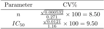
CV coefficient of variation

D drug dose

DIV bolus drug dose

DKL(θ) Kullback-Leibler divergence DSC subcutaneous drug dose

DAISY Differential Algebra for Identifiability of SYstems

DFP Davidon-Fletcher-Powell (algorithm)

DRT dose-response-time

e observed residuals

eij residual variability at timetj for individuali

E(t) drug effect at timet E0 baseline effect Emax efficacy

EAR Exact arithmetic rank

EBE Empirical Bayes Estimates

ED50 potency

EDK50 infusion rate that gives half-measured response EM Expectation-Maximisation

EPO erythropoietin

F bioavailability or biophase availability F(t) FFA concentration at timet

FFA free fatty acids

(11)

FOCEI first-order conditional estimation with interactions

GN Gauss-Newton

H(Ab) drug-mechanism function Hb haemoglobin

HSL hormone sensitive lipase

I(θ) expected Fisher information I( ˆθML) observed Fisher information I(t) insulin concentration at timet IKL(θ) Kullback-Leibler information Imax efficacy (maximal inhibitory effect)

IC50 potency (plasma concentration were 50% of the effect is attained)

ID50 potency (biophase drug amount were 50% of the effect is attained) Inf(t) function dependent on infusion protocol

IR(t) virtual infusion rate at timet IV intravenous

IPRED individual predictions

IWRES individual weighted residuals

k first-order elimination rate

k10 first-order elimination rate from the plasma compartment

k12 first-order distribution rate from the plasma to the tissue compartment k21 first-order distribution rate from the tissue to the plasma compartment ka first-order absorption rate

kag absorption rate from the gut compartment

kasc absorption rate from the subcutaneous compartment ke first-order elimination rate

keo first-order elimination rate from the plasma to the biophase kin turnover rate

koff rate constant for dissociation kon rate constant for association kout fractional turnover rate

kout,max maximal fractional turnover rate ktol fractional turnover rate of moderator Kd dissociation constant

Ki integral gain parameter

Km1 Michaelis constant, first pathway Km2 Michaelis constant, second pathway Kmg Michaelis constant, gut

KM Michaelis constant Kmax maximal toxic effect K-PD kinetic-pharmacodynamic

(12)

KM Levenberg-Marquardt

l(θ;y) log-likelihood function

l(θ,Ω,R;y) population log-likelihood function [L] free ligand concentration

[LR] ligand-receptor complex concentration L(θ;y) likelihood function

L(θ,Ω,R;y) population likelihood function

Lf extendedLie derivative differential operator

L(_fk) k:th repeated Lie derivative M0 moderator baseline

Mi(t) moderator response at timet

MCEM Monte Carlo Expectation-Maximisation

ML maximum likelihood

MM Michaelis-Menten

MSE mean squared error

n number of observations

N number of individuals in the population NiAc nicotinic acid

NLME nonlinear mixed-effects models

ODE ordinary differential equation

p amplification factor

pk search direction

pN

k Newton step

pGN

k Gauss-Newton step

pGN

k Levenberg-Marquardt step

P-P probability-probability

PBPK physiologically-based PK

PD pharmacodynamic

PDE3B phosphodiesterase 3B

PDF probability density function

PK pharmacokinetic

PKA protein kinase A

PL Profile Likelihood

PO per os (Latin for by mouth, i.e., oral drug administration). Q-Q quantile-quantile

QRPEM Quasi-Random Parametric Expectation-Maximisation

[R] free receptor concentration

R residual matrix

R(t) pharmacodynamic response R0 baseline response

b

(13)

RSD relative standard deviation

RSE relative standard error

Smax efficacy (maximal stimulatory effect) Sn(β sum of squares

SA sensitivity analysis

SAEM Stochastic Approximation Expectation-Maximisation

SC subcutaneous

SD50 potency (biophase drug amount were 50% of the effect is attained) SDE stochastic differential equation

STS standard two-stage (method)

SVD singular value decomposition

SYNT endogenous NiAc synthesis

TT x duration of toxic effect

TG triglyceride

ui(t) input functions

V volume of distribution of the drug Vmax maximal elimination rate

Vmax1 maximal elimination rate, first pathway Vmax2 maximal elimination rate, second pathway Vmaxg maximal absorption rate, from the gut Vp volume of distribution, plasma compartment Vt volume of distribution, tissue compartment VPC visual predictive check

x0 initial conditions ˙

xi(t) state variables for theith individual at timet

X design matrix

y dependent variables

yij observations of the system at timestj for individual i

(14)

Acknowledgments

This work would not have been possible without the support and encouragement I have

received during my time as a PhD student. I would first and foremost like to express my

sincerest gratitude to my principal thesis advisors. Thank you, Johan Gabrielsson, for being

an excellent mentor. Besides your experience and vast knowledge in quantitative

pharma-cology, you possess a contagious curiosity of exploring what is unknown to you - a perfect

trait when working in an interdisciplinary field. Thanks to Mats Jirstrand for always being

accessible and sharing your expertise in all aspects of model identification. Your enthusiasm

and compassion contribute to an inspiring and pleasurable working environment. The both

of you have taught me a great deal about how to conduct scientific research. Many thanks to

my advisors at the University of Warwick, Michael Chappell and Neil Evans. Thank you for

providing valuable discussions on model development in general, and identifiability analysis

in particular. Also, big thanks for all of your corrections of my somewhat flawed British

gram-mar. I would like to express my appreciation to Michael for coordinating the IMPACT project.

Many colleagues have aided me in my research. Joachim Almquist at Fraunhofer-Chalmers

Centre is greatly acknowledged for valuable discussions concerning parameter estimation and

parameter uncertainty, and for guidance on the in-house developed Mathematica framework

for nonlinear mixed-effects estimation. Thanks to Christine Ahlstr¨om and Tobias Kroon

at AstraZeneca for generating the data that I have analysed. Thank you, Nick Oakes,

for providing feedback on my pharmacodynamic models and for sharing your insights on

metabolic diseases. I would like to thank my roommates and colleagues David Janz´en and

Linnea Bergenholm who endured spending every waking hour with me in Britain. I would

also like to send my warmest well-wishes to the entire A407 Biomedical Superhero group.

I would not have pursued a research career if it had not been for the support and

(15)

believing in me and my capability.

Me and Tony Johansson have studied together since upper secondary school. Besides

being the closest of friends, you have patiently answered my mathematical queries and

laughed inexplicably at my horrible, stupid humour. Thank you, and good luck on your

future academic career. I would like to thank my dearest friends, Filip and Anton, and the

infamous “You was smoochin’ with my brother!” chat. Thanks to Pablo Lerner for sharing;

intellectual conversations, non-intellectual anti-humour, great taste in music, beers on Andra

L˚ang, among many other things. Thanks to my temporary ‘parents’ Filip and Amanda for

letting me stay at your place.

I would finally wish to express my utmost thanks to my family and all of my friends

for your support through the roller-coaster of ups and downs that constitute the life of a

PhD student.

This work was funded through the Marie Curie FP7 People ITN European Industrial

Doctorate (EID) project, IMPACT (Innovative Modelling for Pharmacological Advances

through Collaborative Training) (No. 316736) and by the Swedish Foundation for Strategic

Research.

Robert Andersson

(16)

Declaration

This thesis have been submitted to the University of Warwick in support of Robert

Anders-son’s application for the degree of Doctor of Philosophy. Robert is the sole author of this

work and it has not been submitted in any previous applications for any degree.

The data presented in this thesis were collected at AstraZenca, Gothenburg, Sweden. The

experimental parts were conducted by Christine Ahlstr¨om Ahlstr¨om et al. (2011b) under the

supervision of Professor Johan Gabrielsson, and by Tobias Kroon Kroon (2016) under the

supervision of Doctor Nicholas Oakes and Professor Johan Gabrielsson.

Parts of this thesis have been published by the author:

[A]Andersson R., Jirstrand M, Peletier L. A., Chappell M. J., Evans N. D., Gabrielsson

J. 2016. Dose-response-time modelling: Second-generation turnover model with integral

feedback control. Eur. J. Pharm. Sci. 81, 189-200.

[B] Andersson R., Kroon T., Almquist J., Jirstrand M., Oakes N. D., Evans N. D.,

Chappell M. J., Gabrielsson J. 2017. Modeling of free fatty dynamics: Insulin and NiAc

(17)

Abstract

The traditional approach to pharmacodynamic modelling relies on knowledge about the

pharmacokinetics. A prerequisite for obtaining kinetic information is reliable exposure data.

However, in several therapeutic areas, exposure data are unavailable—including when the

drug response precedes the systemic exposure (for example pulmonary drug administration)

and when the drug is locally administered (for example ophthalmics).

Dose-response-time (DRT) data analysis provides an alternative to exposure-driven

phar-macodynamic modelling when exposure data are sparse or lacking. In DRT modelling, the

response data are assumed to contain enough information about the drug kinetics, whereby

a biophase model can be developed and act as the driver of the pharmacological response.

The following work presents the fundamental principles of DRT modelling. This include the

entire procedure of identifying a DRT model, encompassing the assessment of the biophase

function and the pharmacodynamic model, extensions to cover population variations,

identi-fiability analysis, parameter estimation, and model validation. To demonstrate the utility of

the technique, two extensive pre-clinical DRT studies of the interaction between nicotinic

acid (NiAc) and free fatty acids (FFA) are presented. The first study covered the response

behaviour following intravenous and oral NiAc dosing in both normal (lean) and diseased

(obese) rats. The second study extended the models of the first study to incorporate insulin

as a driver of the FFA response. Moreover, data from chronic trials were analysed with the

aim to quantitatively understand the adaptive behaviours associated with long-term NiAc

treatments.

The aim of this work is to answer the questions of when and how to use DRT data

(18)

The DRT models of the first study were successfully fitted to all response-time courses

in lean rats, with high precision in the parameter estimates (relative standard errors (RSE)

<25%), visual predictive check (VPC) and individual plots that captured the population and subject trends, andε-shrinkages of less than 10%. The model for the obese rats were less precise, with specific parameters being practically non-identifiable (with, for example,

RSE∼250%). The results for both lean and obese rats were generally consistent with those of

an exposure-driven reference model, albeit with less precision and accuracy in the parameter

estimates. Finally, the model was able to describe non-linear biophase kinetics, present at

high oral dosages of NiAc.

The DRT models of the second study were able to capture the response-time courses

for insulin and FFA on a population and individual level, and for both lean and obese rats.

However, many parameters were uncertain (with RSE of, for example, 30-50%) and some

were practically non-identifiable (with RSE of>100%). The estimates were generally less precise and more inaccurate than those obtained in an exposure-driven reference model.

Yet, most parameter estimates of the DRT models were within one standard deviation from

those of the exposure-driven model. The final model was used to predict steady-state FFA

exposures following repeated NiAc dosing for a range of different infusion protocols. The

optimal dosing regimens consisted of infusions and wash-out periods were the wash-outs

were 2h longer than the infusions. These predictions were consistent with those made by the

exposure-driven model. Albeit, the DRT model predicted a slightly lower optimal reduction

of FFA exposure.

It is important to recognise that DRT analyses introduce bias and variability in the parameter

estimates. To obtain reliable results, it is advisable to have rich pharmacodynamic data,

cover-ing drug administration at different routes, rates, and schedules. With these issues taken into

account, the technique still performed well in the two extensive studies presented in this work.

In conclusion, DRT data analysis is a modelling technique used in situations when

ex-posure data are unavailable. The method is versatile and can describe a range of different

pharmacological behaviours. Precision and accuracy is lost when comparing to an

exposure-driven pharmacodynamic modelling approach. Thus, DRT modelling is not to be considered

as a replacement of the gold-standard pharmacokinetic-pharmacodynamic framework, but

rather as a compliment when exposure data are unavailable.

Keywords: Dose-response-time modelling, Biophase functions, Pharmacodynamic

modelling, Nonlinear mixed-effects (NLME), Disease modelling, Tolerance, Adaptation,

(19)

Part I

(20)

Introduction

This thesis is divided into two parts, each with separate objectives; the first part serves to

describewhat dose-response-time (DRT) data analysis and population modelling are and

how these techniques are applied. The second part focuses onwhy the studies of this PhD

project were conducted, and their respective contribution.

Aims and objectives

The aim of this thesis is primarily to answer the following questions:

• When and how do we use DRT data analysis?

• What are the limitations of DRT data analysis?

In order to achieve the aims, an exhaustive literature review and two major data analyses

were conducted. A key aspect of this project was to demonstrate how simple biophase

structures can be used as the underlying driving mechanism when describing complex

pharmacodynamic systems, where lack of pharmacokinetic data prohibits the standard

pharmacokinetic-pharmacodynamic modelling practice.

Quantitative pharmacology

Modelling and simulation are crucial in modern pharmaceutical research (Allerheiligen, 2014;

Breimer and Danhof, 1997; Burman and Wiklund, 2011; Lalonde et al., 2007; Leil and

Bertz, 2014; Manolis et al., 2013; Marshall et al., 2016; Staab et al., 2013). The methods at

hand provide quantitative ways to perform pharmacology; applicable when evaluating and

comparing drugs, and when designing future experimental protocols (Aarons et al., 2001;

(21)

decisions throughout the drug development cycle, from initialin silico analyses to post-marketing predictive studies on new populations (Bonate, 2011). In detail, modelling and

simulation enable a better understanding of the drug properties, or thepharmacokinetics

(PK) andpharmacodynamics (PD), which are the two main areas of pharmacology (Rowland and Tozer, 2011). PK may in layman’s terms be described aswhat the body does to the drug, which encompasses absorption, distribution, metabolism, and elimination of the drug (Benet

and Zia-Amirhosseini, 1995; Gibaldi and Perrier, 1982). The kinetic properties are assessed

by conducting in vivo studies wherein the drug is administered and the corresponding exposure (typically in blood plasma) is measured over time. The experimental data provide

the basis for the PK model. A well-designed model may contribute quantitative knowledge

of the concentration-elimination relationship, the drug bioavailability, the unbound drug

concentration, the volume of distribution of the drug, and so forth.

In contrast to PK, PD represents what the drug does to the body. Generally, drugs are designed to alter normal physiological or biochemical processes, inhibit pathological

pro-cesses, or disrupt parasites or microbes (Lees et al., 2004). Drugs typically function as

agonists, antagonists or inverse agonists on a specific receptor (Gabrielsson and Weiner,

2010). By binding to its receptor, and forming a receptor-ligand complex, the drug provokes

a stimulating, stabilising or inhibiting action. If the expression of the receptor-ligand complex

is measurable, or some downstream biomarker (Aronson, 2005) is measurable, then the PD

may be assessed. Measuring exposure and drug effect are done in parallel, whereby the drug

concentration-effect relation may be assessed. Traditionally, the PK is analysed first and

considered to drive the PD (Holford and Sheiner, 1982). Consequently, the fitted PK model

will act as the driving mechanism of the perturbed pharmacological response, and the final

PK-PD model will encompass both the kinetic and dynamic properties of the drug and how

these are related.

Dose-response-time data analysis

Dose-response-time data analysis is as an alternative to exposure-driven PK-PD modelling

when PK data are sparse or lacking, or when it is difficult to relate measured exposure

(typically in plasma) to exposure at the target (e.g., in the brain (Andersson et al., 2015;

Gabrielsson et al., 2000; Gabrielsson and Peletier, 2014; Jacqmin et al., 2007)). This

involves studies where, for example, it is undesirable to perform exposure sampling (e.g.,

in paediatrics (Tod, 2008)), the drug is locally administered (e.g. in ophthalmics (Audren

et al., 2004; Gabrielsson et al., 2000; Smolen, 1971b)), general clinical trials (Abou Hammoud

et al., 2009; Buil-Bruna et al., 2014; Ramon-Lopez et al., 2009; Wilbaux and He, 2014),

or the pharmacological response precedes the systemic exposure (e.g. pulmonary drug

administration (Musuamba et al., 2015; Nielsen et al., 2012; Wu et al., 2011)). In DRT

modelling, the pharmacological effect is assumed to be driven by the drug amount at the

(22)

organ, or combinations of tissues and organs. The choice of structure of the biophase depends

on how the drug was administered, what characteristics are seen in the response-time data,

and the physiological knowledge of the system (Andersson et al., 2015; Gabrielsson and

Peletier, 2014).

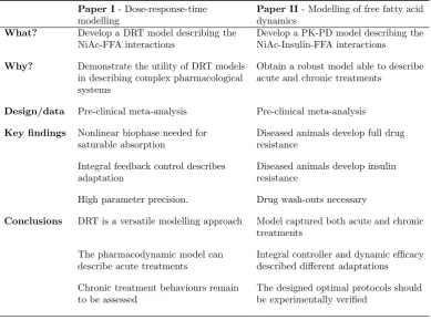
Paper I- Dose-response-time modelling

Paper II- Modelling of free fatty acid dynamics

What? Develop a DRT model describing the

NiAc-FFA interactions

Develop a PK-PD model describing the NiAc-Insulin-FFA interactions

Why? Demonstrate the utility of DRT models in describing complex pharmacological systems

Obtain a robust model able to describe acute and chronic treatments

Design/data Pre-clinical meta-analysis Pre-clinical meta-analysis

Key findings Nonlinear biophase needed for

saturable absorption

Diseased animals develop full drug resistance

Integral feedback control describes adaptation

Diseased animals develop insulin resistance

High parameter precision. Drug wash-outs necessary

Conclusions DRT is a versatile modelling approach Model captured both acute and chronic

treatments The pharmacodynamic model can

describe acute treatments

Integral controller and dynamic efficacy described different adaptations Chronic treatment behaviours remain

to be assessed

[image:22.595.124.514.177.466.2]

The designed optimal protocols should be experimentally verified

Table I: Summary of published articles that are presented in this thesis.

This work provides the principles of DRT data analysis in a population context; how

basic biophase and pharmacodynamic models are constructed, structural and practical

identifiability of these models, incorporation of variability, and assessment of the resulting

models. The technique is demonstrated by means of two pre-clinical meta-analyses. The data

sets for these analyses cover a range of routes, rates, and schedules of drug administration.

Both studies were conducted on the complex metabolic system of free fatty acid (FFA)

dynamics, under the provocation of the antilipolytic compound nicotinic acid (NiAc) (Carlson,

2005). In the first study, the drug dose-response relations are analysed in an acute setting,

using a single-biomarker data set of FFA response-time data. In this study, special emphasis

was placed on the selection process of the biophase functions. The modelled biophase amount

functioned as the driving-mechanism for a sigmoidal function that acted as an inhibiting

force on the turnover of FFA. In the second study, the model was extended to capture chronic

dose-response patterns. This was partly done by adding insulin as a second biomarker.

Two different types of adaptive behaviours were included in the model; one to describe

(23)

available, which allowed for a comparison between the DRT analysis and an exposure-driven

analysis (Andersson et al., 2017; Tapani et al., 2014). The first chapter of the thesis consists of

a thorough literature review of DRT data analysis. This is followed by a Methods and Models

chapter where it is demonstrated how a DRT model is constructed. Furthermore, population

modelling is introduced and, in particular, the nonlinear mixed-effects framework (Bonate,

2011; Davidian, Marie, 2003). This is followed by a section on parameter estimation and

model validation. The second part of the thesis starts with a chapter on the physiology

of NiAc-induced antilipolysis and a presentation of the analysed data. Chapters four and

five consist of the two major case studies where the potential of DRT data analysis is

demonstrated. The majority of the presented scientific contributions have been published

(24)

Chapter 1

Background and literature

review

Pharmacokinetic (PK) and pharmacodynamic (PD) modelling are cornerstones in

model-based drug development. The modelling techniques serve as a means to understanding and

quantifying patterns seen in pharmacological data. This enables the modeller to evaluate

the performance of pharmaceutical substances. Furthermore, suitable models can be applied

to simulate unobserved pharmacological events and thus predict optimal dosage strategies.

In this way, simulations provide valuable input in the design of future experimental trials.

The trials, in turn, contribute new data to be analysed. Hence, mathematical modelling and

simulation and experiments are used symbiotically to enhance the modeller’s knowledge of

the pharmacology and physiology. The iterative strategy of using modelling and simulation

and experiments advances the pharmacological development process until a drug has been

accepted or discontinued.

1.1 PK-PD modelling

The PK-PD modelling procedure is traditionally sequential1 in that the PK are initially

analysed and then considered to be known when assessing the PD. In detail, a PK model

1_{The sequential approach to PK-PD modelling has traditionally been favoured over the simultaneous one}

(25)

is developed and fitted to the exposure-time data (typically drug plasma concentrations).

From the generated PK model, a time continuous exposure signal is generated to act as

an input to the PD model. Consequently, when assessing the PD, it is assumed that the

PK are known and that the simulated PK input corresponds to the true exposure. Given

this premise, the PK-PD modelling framework is constrained by the existence of reliable

exposure data. PKs is often modelled using compartmental models (Godfrey, 1983). These

models consist of ordinary differential equations, where the state variables represent drug

concentrations in different physiological compartments. In the simplest possible case, a

single-compartment model is used to represent the drug concentration in the plasma (model

illustrated in Fig. 1.1a). This concentration, denotedC(t), is given by

dC(t)

dt =−k·C(t) =− Cl

V ·C(t) with C(0) = 0, (1.1)

wherekis the elimination rate,Cl the clearance, andV the volume of distribution of the drug (describing the fraction between the drug amount and the drug concentration2_{). Given}

an intravenous bolus doseD, the initial condition in Eq. (1.1) becomesC(0) =D/V. For extravascular drug administration, an intermediate absorption compartment is added to

Eq. (1.1) from where the drug is absorbed into the blood plasma compartment (model

illustrated in Fig. 1.1b). The drug kinetics are given by

dA(t)

dt =−ka·A(t) with A(0) =D, (1.2a) dC(t)

dt =

F·ka·A(t)

V −k·C(t) with C(0) = 0, (1.2b)

whereA is the drug amount in the absorption compartment,ka the absorption rate, and F the bioavailability. The bioavailability ranges from 0 to 1 and represents the fraction of dose that reaches plasma intact. Generally, Eq. (1.2a) is solved forA(t) and the system is reduced to, and considered as, a single-compartment model given by

dC(t) dt =

D·F·ka·e−kat

V −k·C(t) with C(0) = 0. (1.3)

These elementary PK models may be expanded to include additional compartments,

de-scribing the drug kinetics in other tissues and organs. Such extensions may be required for

various reasons; if, for example there are two different phases in the drug plasma kinetics, the

drug distributes into different tissues, whereby a peripheral compartment is needed (model

illustrated in Fig. 1.1c). In this case, the plasmaCp(t) and tissueCt(t) concentrations after

2_{The volume of distribution is an estimate of how well the drug distributes throughout the body. For}

(26)

a bolus dose could be given by

dCp(t)

dt =k21·Ct(t)−k12·Cp(t)−k10·Cp(t) with Cp(0) =D/V, (1.4a) dCt(t)

dt =k12·Cp(t)−k21·Ct(t) with Ct(0) = 0, (1.4b)

wherek10 is the elimination rate from the plasma compartment,k12 the distribution rate from the plasma to the tissue compartment, andk21 the distribution rate from the tissue to the plasma compartment.

(a) (b) (c)

Figure 1.1: Examples of typical PK models: (a) represents a one-compartment model with first-order drug elimination;(b) a two-compartment model with an absorption and a central drug compartment. The drug is absorbed into, and eliminated from, the central compartment via first-order processes;(c) a two-compartment model with a plasma and a tissue compartment. The drug is distributed between plasma and tissue via first-order processes and eliminated from the plasma via a first-order elimination.

The compartmental modelling framework can be expanded to include any number of

compartments in order to describe more complex kinetic scenarios. In particular, the

physiologically-based PK (PBPK) models consist of multiple compartments and aim at

explaining as much as possible of the drug disposition (Rowland et al., 2011). These

sophis-ticated multi-compartment models provide a more general picture of the drug kinetics, and

are convenient when, for example, translating results between species. However, the scope of

PBPK models often complicates parameter identification (see Section 2.2), and in order for

these models to be useful the modeller generally needs prior knowledge of the pharmacology

and physiology, and/or exposure assays generated at multiple sites (for a review on PBPK

models, see Rowland et al. 2011). As we will see, kinetic information is not always available,

whereby PBPK, and simpler PK models, fail.

1.2 Dose-response-time data analysis

Dose-response-time (DRT) data analysis is a modelling approach that is used for assessing

the PD response when PK data are lacking or uninformative. PK data may, for example, be

(27)

(i) the turnover of the drug is quick (Uehlinger et al., 1992; Port et al., 1998)

(ii) the concentration of the drug is below the limit of quantification (Lalonde and

Gau-dreault, 1999)

(iii) the drug is locally administered (e.g., in ophthalmicss (Audren et al., 2004; Smolen,

1971b; Gabrielsson et al., 2000))

Furthermore, in certain clinical trials, it is undesirable to measure drug exposure due to

the invasiveness of the sampling methods. Invasiveness is generally an issue in paediatric

studies (Tod, 2008) and in situations where the patient is put under considerable

dis-tress (e.g., in oncology (Frances et al., 2011; Paule et al., 2012; Wilbaux and He, 2014)).

Moreover, if the drug effect precedes the systemic exposure (e.g., for pulmonary drug

administration (Musuamba et al., 2015; Nielsen et al., 2012; Wu et al., 2011)), the drug

concentration-time series may be uninformative about the unbound drug at the active site. In

addition, PK data may be uninformative when there are vast differences between the initial

and terminal phase of the drug treatment periods (Lange and Schmidli, 2014, 2015). The

traditional PK-PD modelling approach fails in situations where exposure data are lacking

or uninformative. In cases like these, DRT data analysis acts as a surrogate (a schematic

difference between DRT and PK-PD modelling is illustrated in Fig. 1.2).

DRT modelling is based on the premise that the pharmacological response data contain

information about the drug kinetics. This “hidden” information is assumed to be sufficient

to determine the drug amount in an intermediate biophase compartment. The biophase

represents any organ or tissue where the drug produces its pharmacological effect. From

a modelling perspective, the kinetics of the biophase and the pharmacodynamics need to

be assessed simultaneously, which is not the case in PK-PD modelling. This is achieved by

selecting a possible model that describes the hypothetical drug amount-time course in the

biophase. The biophase amount will subsequently act as the driver of a drug-mechanism

function—which acts on the pharmacological response.

A summary of published DRT data analyses is given in Table 1.1.

1.2.1 Instantaneous response models

Dose-response-time data analysis dates back to the 1960’s and 1970’s when Levy (Levy,

1964a,b, 1966; Gibaldi and Levy, 1972) and Smolen (Smolen, 1971b; Schoenwald and Smolen,

1971; Smolen and Schoenwald, 1971; Smolen, 1971a; Smolen and Weigand, 1973; Smolen

et al., 1975; Smolen, 1976b,a,c, 1978) introduced the concept. Levy described a relationship

between the amount of drug in the body and the corresponding pharmacological effect.

Smolen, on the other hand, analysed the dose-response relationship of a mydriatic3 _drug

after oral and ophthalmic administration. In the qmydriatic studies, no exposure data were

available due to difficulties in assaying the drug in body fluids. Consequently, response

(28)

PK-PD modelling approach

[image:28.595.152.474.133.390.2]

DRT modelling approach

Figure 1.2: Illustration of the conceptual difference between traditional PK-PD modelling and DRT analysis. In traditional pharmacodynamic modelling, the response is assumed to be driven by the pharmacokinetic model. In DRT modelling, the response is driven by the drug amount in the biophase.

data were the sole source of information when quantifying the bioavailability and biokinetic

behaviours. Smolen’s studies were based on two major assumptions (Smolen, 1976c):

• “The dynamics of the drug’s disposition are linear.”

• “The intensity of pharmacological response is a single-valued function of the biophasic drug levels.”

For example, with a biophase amount of Ab(t), and a pharmacological response of I(t) (mydriatic response intensity, in this case), the functional relationship was assumed to be

given by

I(t) =f(Ab(t)), (1.5)

for some appropriate functionf. Now, given the first assumption, a dose vs. effect relationship was used to convert observed intensity-time courses into relative biophase amount-time

courses. Combining this with a compartmental model for the biophase dynamics, and

(29)

Smolen analysed a range of two- and three-compartment biophase models to describe the

kinetics of the biophase (the are models illustrated in Fig. 1.3). The corresponding model

fits demonstrated the structural and practical identifiability4_{issues associated with}

multi-compartment biophase models (without making appropriate prior assessments). Nonetheless,

when applying an identifiable biophase function, the method was proven to be successful in

capturing the pharmacodynamic behaviours and the biophase kinetics. However, the second

of Smolen’s assumptions heavily constrains the application of the defined technique since

many pharmacological processes are non-direct (Dayneka et al., 1993).

Figure 1.3: Biophase models presented by Smolen (1971b). Smolen used two-compartment models with a biophaseAb, and systemic fluidAc compartment, and three-compartment models with a biophase Ab, a systemic fluid Ac, and a tissue depot compartment Ad. Moreover, a fourth compartment Aa, corresponding to the site of administration, was included if the drug was not administered systemically.

Since those initial studies, DRT modelling was not applied until the early 1990’s when Verotta

and Sheiner (1991) further developed the existing techniques. In their study, semi-parametric

methods were applied to analyse pharmacodynamic data over a range of different data sets

(e.g., verapamil-induced changes in the PR interval of an electrocardiogram). Verotta and

Sheiner (1991) made the following model assumptions

• “Both the distribution of the drug and its effect vs. concentration relationship are stationary processes.”

• “The distribution of the drug is linear with respect to the input of the drug.”

• “The pharmacodynamic response to the drug depends on the concentration of the drug

at a single site.”

• “The relationship between effect and drug concentration is memoryless.”

4_{The identifiability issues were discussed by Smolen. However, no formal identifiability analysis was}

(30)

The semi-parametric model consisted of an unobserved stateX that was proportional to the drug concentration at the active siteCe. The stateX was given by the convolution of the input function and a sum of exponentials. Furthermore, the pharmacological effectE was related to X according to a cubic spline. As Verotta and Sheiner had access to PK data in their study, the estimated exposure could be compared with the observed exposure.

Here, the uncertainty of the non-parametric technique was made clear, as the worst case

estimated exposure profile was far off the observed exposure. Furthermore, the assumption

of having stationary processes and a memoryless relationship between the effect and the

drug concentration limits the method substantially. However, the study by Verotta and

Sheiner inspired subsequent DRT studies. In particular, the response behaviour of the

muscle relaxant drug vecuronium was analysed in a range of studies (Bragg et al., 1994;

Fisher and Wright, 1997; Fisher et al., 1997; Warwick et al., 1998), where twitch depressions

of the muscles were used as the pharmacodynamic biomarker. In these studies, the drug

plasma concentration was measurable, but not the concentration at the neuromuscular

junction, which is the effective site. Regardless, the studies successfully characterised both

the respiratory and adductor pollicis muscle behaviours seen after vecuronium administration.

This was done by modelling the biophase concentration Ce (called effective concentration or

active concentration in the studies) with a first-order elimination model given by

Ce =keo·D·

A·(e−λt₋_e−keot₎ keo−λ

, (1.6)

wherekeo is the elimination rate from the plasma compartment to the biophase compart-ment,D is the dose,Athe dose-normalised intercept, andλthe elimination rate from the biophase compartment. This biophase concentration drives the response according to a Hill

equation (Gesztelyi et al., 2012)

Effect = Ce

γ

Ceγ+ Cγ₅₀, (1.7)

where C50 is the steady-state concentration that produces 50% of the effect, andγ is the Hill coefficient. This model was applied to both the respiratory and the adductor pollicis

twitch tension data. The models showed that the peak concentration of vecuronium occurred

earlier in the respiratory muscles than in the adductor pollicis. This implies a higher peak

concentration level and thus explains why the respiratory muscles more frequently experience

paralysis than the adductor pollicis after vecuronium exposure. Furthermore, Warwick et al.

(1998) showed the potential advantages associated with PK-free PD analysis. In particular,

the DRT approach allows for individual predictions of future dosing during anaesthesia. This

is not possible using the conventional PK/PD approach due to the time needed to assay the

drug. Further usage of DRT data analysis was successfully demonstrated in studies where

children were treated with erythropoietin (EPO) for renal anaemia (Uehlinger et al., 1992;

(31)

linearly dependent on the EPO dose

R=β·D, (1.8)

whereR is the drug-induced Hb production,Dthe dose, andβ the production rate per dose unit. A DRT approach was suitable in these studies since the EPO turnover is rapid in

comparison to the response turnover. Consequently, it is hard to relate the concentration-time

course of EPO to that of Hb.

1.2.2 Turnover models

Following the DRT studies of the 1990’s, the field saw a breakthrough when Gabrielsson

et al. (2000), introduced biophase-driven turnover models (Dayneka et al., 1993). In the

turnover model framework, the PD responseR(t) is given by

dR(t)

dt =kin−kout·R(t) with R(0) =R0, (1.9)

wherekinandkout are the turnover and fractional turnover rate of the response, respectively, andR0 is the baseline response. For a biophase-driven response, the biophase amountAb will act on the production or elimination of response through a drug-mechanism function

H(Ab) according to

dR(t)

dt =kin·H(Ab)−kout·R(t) (1.10)

or

dR(t)

dt =kin−kout·H(Ab)·R(t). (1.11)

The drug-mechanism functions that were applied in the study by Gabrielsson et al. (2000)

included nonlinear Hill relations (similar to that of Eq. 1.7) that were either stimulatory

H(Ab) = 1 +

Emax·Aγ_b

ED₅₀γ +Aγ_b (1.12)

or inhibitory

H(Ab) = 1− Emax·A

γ

b

ED₅₀γ +Aγ_b. (1.13)

where Emax is the efficacy, ED50 the potency (based on dose), and γ the Hill coefficient. Turnover models allow for a wide range of response-time behaviours, out of the scope of

previous DRT studies (due to their assumptions). The study by Gabrielsson et al. (2000),

contained four different cases of biophase-driven turnover models, describing response-time

(32)

is illustrated in Fig. 1.4). These case studies showed that DRT models are applicable when

the kinetics and/or dynamics behave non-linearly, when there are time-delays in the response

data, and when the system contains feedback mechanisms. This heavily expanded the

possible applications of DRT models. Beyond the study of Gabrielsson et al. (2000), the

Figure 1.4: Biohase-driven turnover model presented by Gabrielsson et al. (2000). The input into the biophase is either direct (iv administration) or through absorption (oral administration)F·ka, whereF is the biophase availability andkais the first-order absorption rate from an absorption compartment into the biophase. The parameterk is the first-order (linear) elimination rate from the biophase. The biophase amount Ab was then driving a drug-mechanism function H(Ab), which can, for example, inhibit the turnover kin or fractional turnoverkoutof the response R.

biophase-driven turnover model was applied across a range of DRT studies in the late 1990’s

and early 2000’s (Lalonde and Gaudreault, 1999; Audren et al., 2004; Gruwez et al., 2005; Tod

et al., 2005). In particular, Lalonde and Gaudreault (1999), analysed parathyroid hormone

concentrations under treatment by the calcimimetic agent R-568. Since the concentration

of the specific agent was below the limits of quantification in more than half of the patient

samples, the exposure analysis was excluded and the PD model was assumed to be driven

by the drug amount in the biophase. Further, Gruwez et al. (2005) applied a dose-response

model to analyse categorical data when they explored the effect of paroxetine and pindolol.

Here, the response-time data consisted of total scores on the MADR scale (Montgomery and ˚

Asberg, 1979).

1.2.3 Kinetic-Pharmacodynamic models

In addition to the original DRT-approach by Smolen (1971b), an alternative rate-driven

model (K-PD) was suggested by Jacqmin et al. (Gieschke et al., 2001; Goggin et al., 2001;

Jacqmin et al., 2001; Pillai et al., 2001). The concepts of the K-PD model are similar to

(33)

rate) is assumed to be the driver of the pharmacological response, rather than the biophase

amount. This is an unconventional approach in pharmacological modelling, where drug

exposure (or amounts) are generally assumed to drive the pharmacological effect.

To demonstrate the idea of the K-PD model, assume that the biophase amountAb(t) has a first-order elimination ratek given by

dAb(t)

dt =−k·Ab(t), (1.14)

with initial valueAb(0) =D. Furthermore, assume that the drug inhibits the turnover of the pharmacodynamic responseR(t) according to a nonlinear Hill relation. The response behaviour would then, for the traditional DRT and the K-PD approach, be given by

dR(t)

dt =kin· 1−

Emax·A

γ

b(t) ED₅₀γ +Aγ_b(t)

!

−kout·R(t) DRT, (1.15)

and

dR(t)

dt =kin· 1−

Emax·IRγ(t) EDK₅₀γ +IRγ₍_t₎

!

−kout·R(t) K-PD, (1.16)

with

IR(t) =−dAb(t)

dt =k·Ab(t), (1.17)

whereIR(t) is the virtual infusion rate andEDK50(amount per time unit) the rate that gives half-measured drug-reduced response. As is indicated by Eq. (1.17), the ‘drivers’ of the

DRT and K-PD models are proportional. Thus, the two frameworks only differ by a scaling

factor.

K-PD models have been applied in numerous studies (see for example Abou Hammoud et al.

(2009); Hamberg et al. (2013); Salem et al. (2016); Wu et al. (2011)) following its introduction

by Jacqmin et al. (2001, 2007). However, several studies have misunderstood the original

model definition and used the biophase amount as the driving force of the response (see

for example Gruwez et al. (2007); Jacobs et al. (2010); Mikaelian et al. (2013); Musuamba

et al. (2015); Nielsen et al. (2012)). These studies have in fact applied the traditional DRT

approach (Smolen, 1971b).

In a study of chemoradiotherapy-induced thrombocytopenia by Krzyzanski et al. (2015), no

biophase kinetics were addressed. Rather, the drug (carboplatin) was assumed to have an

on/off effect given by

T x(t) =



 

 

Kmax if tj≤t≤tj+TT x,

0 otherwise,

(34)

that acted on the elimination of cells. Here,tjrepresents the starting time of the chemora-diotherapy,TT x the duration of the toxic effect andKmaxis the maximal toxic effect. The study by Krzyzanski et al. (2015) demonstrated that DRT modelling does not necessarily

need to include a compartmental biophase.

1.3 Summary and perspectives

DRT data analysis could be an option when the traditional PK-PD approach fails. This

occurs when exposure data are lacking or are uninformative, which may be due to:

• Exposure sampling is difficult—quick drug turnover, drug concentrations below limits of quantification, local administration etc.

• Exposure sampling is undesirable—clinical studies, in particular within paediatrics.

• Exposure data are uninformative about the drug exposure—e.g., pulmonary

adminis-tered drugs or drugs that penetrate the blood-brain barrier.

• Large time differences between the initial and terminal phase—biologics (Morrow and Felcone, 2004).

The technique has been applied for describing drug behaviour in several therapeutic areas

(see Table 1.1). In almost all of these studies, simple biophase models were used with

first-order elimination and first-order absorption (the latter being applied in cases where

drug is not directly administered into the biophase). During recent years, DRT modelling

has frequently been applied in clinical oncology (Buil-Bruna et al., 2014; Frances et al., 2011;

Parra-Guillen et al., 2013; Paule et al., 2012; Ramon-Lopez et al., 2009; Wilbaux and He,

2014)—a therapeutic area where invasiveness is undesirable. As for clinical oncology studies,

invasiveness is an issue in paediatric studies. Thus, DRT modelling is a promising technique

(35)

(36)

(37)

(38)

[image:38.595.182.450.104.750.2]

(39)

Chapter 2

Methods and models

This chapter serves to illustrate how to perform dose-response-time (DRT) data analysis.

In principle, the study constitutes five fundamental modelling techniques; model selection,

identifiability analysis, parameter fitting, sensitivity analysis, and modelevaluation. These

techniques will be examined in a logical order—albeit remembering that modelling is an

iterative exercise where the modeller goes back and forth until the final model meets some

quantitative or qualitative criteria. Since the methods ultimately are designed to be applied

in pharmacological studies, particular focus will be on the implementation of the ideas in

various examples.

The first section of this chapter covers model selection in a standard DRT data analysis—

wherein mean population behaviours are described. Central to these studies is the choice

of the biophase function. The biophase generally has a basic structure with, for example,

zero- or first-order drug absorption and first-order drug elimination from the biophase. The

modelled drug amount in the biophase is subsequently assumed to act as the driver of

the pharmacological response via a drug-mechanism function. To successfully choose the

PD model with a suitable drug-mechanism function, the response-time data need to be

qualitatively analysed and the characteristic response behaviours recognised. The second

section of the chapter is devoted to population modelling, where it is demonstrated how a

biophase-driven PD model may be extended to incorporaterandom effects. These allow for a quantitative way to assess differences in a population, such as between-subject, inter-study,

and inter-occasional variabilities (Bonate, 2011; Davidian, Marie, 2003). To determine

(40)

to vary in populations (Mould and Upton, 2012). The section will mainly focus on the

nonlinear mixed-effects frameworksince this has been the standard population modelling

approach in pharmacology for more than 30 years (Sheiner and Beal, 1980, 1981, 1983). In

the subsequent section, the developed models will be subject to an identifiability analysis

to verify that the parameter estimation problems are well-posed (Raue et al., 2014). The

discussion will encompass both a priori and data-based identifiability techniques. The identifiability analysis is followed by a section on different methods for parameter estimation,

particularly for nonlinear mixed-effects models. The fourth section will cover sensitivity

analysis; a framework that studies how the system output is affected by uncertainties, or

perturbations, of the input. Sensitivity analysis techniques will be proven to be useful in both

model selection and validation. Finally, tools for validation and diagnostics are examined as

ways for quantitative and qualitative evaluation of the analysis.

2.1 Model selection

One of the biggest challenges of developing a DRT model is that the biophase dynamics and

the PD need to be assessed simultaneously. Consequently, it may be difficult to distinguish

the kinetic and dynamic properties of the drug from each other. More specifically, time-delays

in the dose-response data could, for example, be a consequence of rate-limiting absorption or

slow onset of the biomarker. To discriminate between the kinetic and dynamic properties, it

is important to have arich1 _{data set. The data should preferably include multiple dosages} and administration routes, as well as careful selection of the dosages (Gabrielsson et al.,

2000).

2.1.1 Biophase function

The biophase model is generally simple due to the difficulties associated with identifying

a complex kinetic model without exposure data (for identifiability analysis, see Sec. 2.2).

More sophisticated biophase models may be used by making prior assessments and fixing

some parameter values. The simplicity of the single–compartment biophase model makes

it a suitable candidate for describing the biophase dynamics. This model will be slightly

modified depending on the drug administration route. If the drug enters directly into the

biophase, the input function is that of an intravenous (IV) administration. With a first-order

elimination rate from the biophase, denoted byk, the dynamics of the biophase following a direct bolus input or an infusion input are given by

dAb(t)

dt =−k·Ab(t) with Ab(0) =D bolus, (2.1)

1_{Obtained from experiments where the system has been properly ‘provoked,’ thereby revealing the full}

(41)

or

dAb(t)

dt = Inf(t)−k·Ab(t) with Ab(0) = 0 infusion, (2.2)

whereAb(t) is the biophase drug amount, Inf(t) a function dependent on the infusion protocol, D the drug dose (the models are illustrated in Fig. 2.1a and Fig. 2.1c, respectively). If

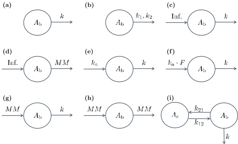
(a) (b) (c)

(d) (e) (f )

[image:41.595.138.523.214.447.2]

(g) (h) (i)

Figure 2.1: Examples drawn from the biophase model library: (a) represents a bolus input and first-order elimination; (b) a bolus input and biphasic first-order elimination; (c) a zero-order input and first-order elimination; (d) a zero-order input and Michaelis-Menten elimination; (e) a first-order input and elimination; (f) a first-order input, scaled by the biophase availability, and order elimination; (g) Michaelis-Menten input and first-order elimination; (h) Michaelis-Menten input and elimination; (i) two-compartment model with order distribution between the central compartment and the biophase and first-order elimination from the biophase. The parametersAb, Inf,k,ka,F and MM represent, respectively, the biophase amount, the constant rate infusion input, the first-order elimination rate constant, the first-order absorption rate constant, the biophase availability and the Michaelis-Menten absorption/elimination process, respectively. All models presented in the library have been applied in published DRT studies (see Table 1.1)

the drug is administered to a peripheral compartment, and subsequently absorbed into the

biophase via a first-order process, then the biophase dynamics are given by

dAa(t)

dt =−ka·Aa(t) with Aa(0) =D, (2.3a) dAb(t)

(42)

whereAa(t) is the drug amount in the absorption compartment,kathe first-order absorption rate into the biophase, andF the availability, or thebiophase availability (Smolen (1971b), model illustrated in Fig. 2.1e). By solving forAa(t) in Eq. (2.3a), the system can be re-written as

dAb(t)

dt =D·F·ka·e

−kat₋_k_·_A

b(t) with Ab(0) = 0. (2.4) The aforementioned models are the simplest biophase functions and these have been frequently

applied in DRT studies (see Table 1.1). Apart from these models, Andersson et al. (2015)

introduced nonlinear absorption/elimination models to describe the biophase dynamics.

In their study, an extravascular doseD was absorbed into the biophase via a nonlinear Michaelis-Menten model, which gives the following biophase dynamics

dAa(t) dt =−

Vmax·Aa(t) Km+Aa(t)

with Aa(0) =D, (2.5a)

dAb(t) dt =

Vmax·Aa(t) Km+Aa(t)

−k·Ab(t) with Ab(0) = 0, (2.5b)

where Vmax is the maximal absorption rate from the absorption compartment andKm the drug amount at which 50% absorption is attained. The biophase elimination could, of course,

also be modelled using the nonlinear Michaelis-Menten model. A typical scenario is that the

drug amount (or concentration) is measurable in a central compartment (e.g., plasma) but

not in the biophase. In cases like these, multi-compartmental biophases could be applied.

Such a model could, for example, be characterised in the following way:

dAb(t)

dt =k12·Ac(t)−k21·Ab(t)−k·Ab(t) with Ab(0) =D, (2.6a) dAc(t)

dt =k21·Ab(t)−k12·Ac(t) with Ac(0) = 0, (2.6b)

where Ac(t) is the drug amount in a central compartment,k12 andk21 are the absorption/e-limination rates between the biophase and central compartment,kthe elimination rate from the biophase out of the system, and D the drug amount (model illustrated in Fig. 2.1i). Models like the aforementioned have been used by Fisher et al. (1997) among others (Smolen,

1971b; Warwick et al., 1998).

2.1.2 Pharmacodynamic model

The pharmacology literature encompasses a plethora of PD models—aimed at describing

different pharmacological phenomena. This section will cover the ones most commonly

applied in DRT studies. This includes, for instance, direct and indirect models with linear

and nonlinear dose-response relations. For a more thorough discussion on PD modelling, see

for example Gabrielsson and Weiner (2010).

The PDs in the DRT framework are assumed to be driven by the biophase amountAb(t). If there is a rapid equilibrium between the biophase amount and the pharmacological effect

(43)

2010). The simplest possible direct response model assumes a linear effect-amount relation

given by

E(t) =E0±β·Ab(t), (2.7)

whereE(t) is the effect, E0 the baseline, andβ the slope parameter. However, the linear dose-response relationship is unbounded and therefore violates basic physiological principles

(e.g., a limited receptor pool). TheEmax model, on the other hand, has a saturable dose-response relationship as well as physiologically interpretable parameters (Gabrielsson and

Weiner, 2010). The standard (γ= 1) and sigmoidal form of this model are given by

E(t) =E0±

Emax·A

γ

b(t)

EDγ₅₀+Aγ_b(t), (2.8)

whereEmaxis the maximal drug effect (efficacy),ED50 the biophase drug amount at 50% maximal effect (potency), andγ the Hill exponent. The linear and saturable direct response models in Eqs. (2.7) and (2.8) have been applied in several DRT studies (Uehlinger et al., 1992;

Port et al., 1998; Bragg et al., 1994; Fisher et al., 1997; Fisher and Wright, 1997; Warwick

et al., 1998). To illustrate the connection between the Emax-model and ligand-receptor binding, consider thelaw of mass action, which states

[L] + [R]

kon

koff

[LR], (2.9)

where [L] is the free concentration of a specific ligand, [R] the free concentration of the corresponding receptor, [LR] the free concentration of the receptor-ligand complex, kon the rate constant for association, andkoff the rate constant for the dissociation. For the receptor-ligand binding, assume that

• The interaction is reversible.

• The interaction is rapid.

• The receptor has one binding site for the ligand.

• The receptor, ligand, and receptor-ligand complex are in equilibrium.

Under equilibrium, Eq. (2.9) implies that

kon[R][L] =koff[LR], (2.10)

or

[R][L] [LR] =

koff kon

(44)

whereKdis known as the the dissociation constant. Now, assume that a drug-induced effect is proportional to the free concentration of the receptor-ligand complex as

E=α·[LR]. (2.12)

This implies that the maximal drug-induced effect is given by

Emax=α·([LR] + [R]). (2.13)

By taking the fraction of the drug-induced effect and the maximal effect, we get

E Emax

= [LR]

[LR] + [R] (2.14) = 1

1 + _[_LR[R]_]

. (2.15)

Using the identity in Eq. (2.11) gives

E Emax

= [L] [L] +Kd

(2.16)

or

E= Emax·[L] [L] +Kd

, (2.17)

and we are done. To conclude, under some assumptions, theEmax-model may be derived from the law mass action of receptor-ligand binding.

The previous discussion has focused on direct response models. Generally though, the

relationship between the biophase drug amount and the pharmacological effect is indirect,

whereby turnover models are frequently applied (Dayneka et al., 1993). In a turnover model,

the responseR(t) is given by

dR(t)

dt =kin−kout·R(t) with R(0) =R0, (2.18) wherekin andkout are the turnover rate and the fractional turnover rate of the response, respectively, andR0the baseline response. Depending on the nature of the drug, its induced effect is typically given by a drug-mechanism functionH(Ab(t)) that is either stimulatory

H(Ab(t)) =S(Ab(t)) = 1 +

Smax·Aγb(t) SD₅₀γ +Ab(t)γ

, (2.19)

or inhibitory

H(Ab(t)) =I(Ab(t)) = 1−

Imax·Aγ_b(t)

(45)

Here,Smaxand Imax represent the maximum stimulatory and inhibitory effect (efficacies), respectively,SD50andID50are the biophase drug amounts were 50% of the effect is attained (potencies), andγis the Hill exponent. The stimulatory (displayed in Eq. (2.19)) or inhibitory (displayed in Eq. (2.20)) drug effect acts on the production or loss (or both) of response

in Eq. (2.18). For example, a stimulatory effect on the turnover would yield the following

relation:

dR(t)

dt =kin·S(Ab(t))−kout·R(t), (2.21) and an inhibitory effect on the fractional turnover would be given by

dR(t)

dt =kin−kout·I(Ab(t))·R(t). (2.22)

Turnover equations with nonlinear inhibition or stimulation have frequently been applied in

DRT studies (see for example Abou Hammoud et al. (2009); Audren et al. (2004); Lalonde

and Gaudreault (1999); Gabrielsson et al. (2000); Mikaelian et al. (2013); Wilbaux and He

(2014)).

Example 2.1.2.1 Turnover model (Gabrielsson et al., 2000)

In order to illustrate how the characteristic behaviours of a generic response-time

data set are extracted, consider the following example where an antinociceptive drug has been

given both as an IV bolus (in two different doses of 40 and 80µg kg−1) and subcutaneously

(in three different doses of 50, 100, and 200µg kg−1_{) to Sprague-Dawley rats (the data are}

adapted from Gabrielsson et al. (2000)). Post drug administration, radiant heat is focused

on the tail of the rat and the time, in seconds, is measured until the rat removes its tail. The

response-time behaviour was observed during 180 min (the data are illustrated in Fig. 2.2).

Since the drug was administered via two different routes, we need two separate biophase

● ● ●

● ●

●

■■ ■

■ ■

■

◆ ◆

◆

▲ ▲

▲

▲ ▲

▼▼ ▼

▼ ▼

▼

0 50 100 150 200

0 2 4 6 8 10 12 14

●

■

◆

▲

▼

Dose response time data analysis

A Thesis Submitted for the Degree of PhD at the University of Warwick

Permanent WRAP URL:

http://wrap.warwick.ac.uk/100470/

Copyright and reuse:

This thesis is made available online and is protected by original copyright.

Please scroll down to view the document itself.

Please refer to the repository record for this item for information to help you to cite it.

Our policy information is available from the repository home page.

Dose-response-time data analysis

Karl Robert Andersson

Thesis

Submitted to the University of Warwick

for the degree of

Doctor of Philosophy in Engineering

Biomedical and Biological Systems

School of Engineering

University of Warwick

Table of Contents

I

Introduction

1

II

Analysis and results

72

List of Figures

List of Tables

Abbreviations and symbols

Acknowledgments

Declaration

Abstract

Part I

Introduction

Aims and objectives

Quantitative pharmacology

Dose-response-time data analysis

Chapter 1

Background and literature

review

1.1

PK-PD modelling

1.2

Dose-response-time data analysis

1.2.1

Instantaneous response models

1.2.2

Turnover models

1.2.3

Kinetic-Pharmacodynamic models

1.3

Summary and perspectives

Chapter 2

Methods and models

2.1

Model selection

2.1.1

Biophase function

2.1.2

Pharmacodynamic model