warwick.ac.uk/lib-publications
Original citation:
Seresinhe, Chanuki Illushka, Preis, Tobias and Moat, Helen Susannah. (2017) Using deep
learning to quantify the beauty of outdoor places. Royal Society Open Science, 4 (7). 170170.
Permanent WRAP URL:
http://wrap.warwick.ac.uk/91136
Copyright and reuse:
The Warwick Research Archive Portal (WRAP) makes this work of researchers of the
University of Warwick available open access under the following conditions.
This article is made available under the Creative Commons Attribution 4.0 International
license (CC BY 4.0) and may be reused according to the conditions of the license. For more
details see:
http://creativecommons.org/licenses/by/4.0/
A note on versions:
The version presented in WRAP is the published version, or, version of record, and may be
cited as it appears here.
rsos.royalsocietypublishing.org
Research
Cite this article:Seresinhe CI, Preis T, Moat
HS. 2017 Using deep learning to quantify the
beauty of outdoor places.R. Soc. open sci.
4: 170170.
http://dx.doi.org/10.1098/rsos.170170
Received: 23 February 2017 Accepted: 19 June 2017
Subject Category:
Computer science
Subject Areas:
environmental science/computer modelling and simulation
Keywords:
environmental aesthetics, well-being, convolutional neural networks, deep learning, online data
Author for correspondence:
Chanuki Illushka Seresinhe
e-mail:[email protected]
Electronic supplementary material is available
online at https://dx.doi.org/10.6084/m9.
figshare.c.3817837.
Using deep learning to
quantify the beauty of
outdoor places
Chanuki Illushka Seresinhe
1,2
, Tobias Preis
1,2
and
Helen Susannah Moat
1,2
1Data Science Lab, Behavioural Science, Warwick Business School, University of
Warwick, Coventry CV4 7AL, UK
2The Alan Turing Institute, British Library, 96 Euston Road, London NW1 2DB, UK
CIS,0000-0001-6599-1325; TP,0000-0001-9185-0892; HSM,0000-0001-8974-9277
Beautiful outdoor locations are protected by governments and have recently been shown to be associated with better health. But what makes an outdoor space beautiful? Does a beautiful outdoor location differ from an outdoor location that is simply natural? Here, we explore whether ratings of over 200 000 images of Great Britain from the online game Scenic-Or-Not, combined with hundreds of image features extracted using the Places Convolutional Neural Network, might help us understand what beautiful outdoor spaces are composed of. We discover that, as well as natural features such as ‘Coast’, ‘Mountain’ and ‘Canal Natural’, man-made structures such as ‘Tower’, ‘Castle’ and ‘Viaduct’ lead to places being considered more scenic. Importantly, while scenes containing ‘Trees’ tend to rate highly, places containing more bland natural green features such as ‘Grass’ and ‘Athletic Fields’ are considered less scenic. We also find that a neural network can be trained to automatically identify scenic places, and that this network highlights both natural and built locations. Our findings demonstrate how online data combined with neural networks can provide a deeper understanding of what environments we might find beautiful and offer quantitative insights for policymakers charged with design and protection of our built and natural environments.
1. Background
Governments around the world spend a great deal of money preserving and creating beautiful places [1]. As individuals, we often seek such locations out when desiring rest and relaxation. However, the beauty of outdoor spaces has long been considered an intangible measure that is difficult to quantify due to its subjective nature. Outdoor beauty is often considered synonymous with ‘nature’, as evidenced by the
2
rsos
.ro
yalsociet
ypublishing
.or
g
R.
Soc
.open
sc
i.
4
:1
70
170
...
major efforts taken to preserve areas in the countryside [2] such as Outstanding Areas of Natural Beauty, and the plethora of landscape paintings presented in museums. Yet, should we deem all natural areas worthy of protection? What about areas that are not primarily natural? What environments in towns and cities might also be considered beautiful, and thus worthy of preservation? If we can quantify the beauty of outdoor spaces, we can find answers to such questions.
While individual ideas of beauty are likely to be shaped by our personal cultural and social experiences, there is also reason to believe that our preferences for certain environments are shaped by evolution [3–5]. Such preferences may not only be for natural elements [6,7], but also for areas with wide vantage points [3], moderate levels of complexity [8–10] and enclosedness [11]. Thus, it is feasible to suppose that there is a collective sense of beauty that we can measure, and that this may not in fact coincide wholly with only natural beauty.
Traditionally, small-scale surveys have been the most cost-effective method of gathering quantifiable data on what people find beautiful in outdoor spaces. Such surveys have provided important initial evidence that beautiful spaces may encourage physical activity [12,13]. However, small-scale surveys have limited scope in terms of which characteristics of environments they can explore, and have generally only explored a handful of characteristics at a time, such as the presence of natural elements [14–16], fractal elements [17,18] or complexity [8–10].
The ability to crowdsource large amounts of data, coupled with recent advances in computer vision methods, is opening up a new avenue for research, allowing us to investigate visual perceptions of our environment. A recent analysis of over 1.5 million ratings of over 200 000 outdoor images taken across Great Britain, crowdsourced via the online gameScenic-Or-Not,provided evidence that people who live in more scenic environments report their health to be better [19]. Crowdsourcing has also been used to collect large databases of human perceptions of city images such as ‘safety’, ‘beauty’ and ‘happiness’ [20,21]. Computer vision methods such as ‘sparse coding’ [22] and ‘bag of visual words’ [23] have allowed researchers to identify statistical characteristics and specific areas of images that relate to concepts such as ‘artistic style’ [24] or visual perceptions of cities [25]. More recently, the introduction of convolutional neural networks (CNNs) has led to dramatic improvements in computer vision tasks, including visual recognition [26,27], understanding image aesthetics [28,29] and extracting perceptions of urban neighbourhoods [30,31].
We draw on this ongoing and rapid improvement in computer vision, particularly with CNNs. We use the Places CNN [32,33] to extract hundreds of features from over 200 000 outdoor images from across Great Britain, rated via the online gameScenic-Or-Not, in order to develop a deeper and broader understanding of what beautiful outdoor spaces are composed of. We attempt to find answers to our question that go beyond the simple explanation ‘what is natural is beautiful’. Finally, we evaluate to what level of accuracy we can create a model to predict the beauty of scenes for which we do not have survey or crowdsourced scenicness data.
2. Exploring the composition of beautiful outdoor scenes
3
rsos
.ro
yalsociet
ypublishing
.or
g
R.
Soc
.open
sc
i.
4
:1
70
170
...
We use the more recent Places365 CNN trained on the Places2 dataset (a repository of 8 million scene photographs) [33] to extract the probabilities of 365 place category classifications such as ‘mountain’, ‘lake natural’, ‘residential neighbourhood’ and ‘train station platform’. We specifically use the Places365 trained using the 152-layer Residual Network (ResNet152) architecture [37], as this resulted in the best classification accuracy. Table S2 in the electronic supplementary material lists all place categories used in our analysis.
We also explore the basic characteristics of photographs in our scenic ratings dataset, including their colour composition, saturation, brightness and colour variations. We examine each image from Scenic-Or-Not on a per-pixel level, with each pixel being allocated to one of 11 colours that constitute the principal colours in the English vocabulary (black, blue, brown, grey, green, orange, pink, purple, red, white and yellow). More details of this procedure and the empirical data that support it can be found in the electronic supplementary material.
Visual inspection of a sample of the most highly scenic images suggests that they conform to widely held notions of beautiful scenery, comprising rugged mountains, bodies of water, abundant greenery and sweeping views (figure 1a). The sample of least scenic images suggests that such images are often composed of primarily man-made objects such as industrial areas and highways. However, images containing large areas of natural greenery can also be considered unscenic if they look drab, or if man-made objects, such as industrial plants, are obstructing the view (figure 1b).
We also look at a subset of images that are located in urban areas and do not consist primarily of natural land cover that might be associated with beautiful scenery. We differentiate urban areas from rural areas using area classification data from national statistics sources [38,39]. We use data on land cover from the25 m-resolution UK Land Cover Map 2007 (LCM)[40] to identify images that are located in primarily built-up rather than natural areas. Table S3 in the electronic supplementary material lists which land cover types have been deemed natural versus built-up.
The sample of images we inspect suggests that the definition of scenicness in urban built-up settings is more varied than in rural areas (figure 1c). It appears that the most scenic images in urban areas consist not only of images that might be reminiscent of countryside scenery—such as beautiful canals and tree-lined paths—but of images that also contain man-made features such as historical architecture and bridge-like structures.
The number of photographs in our dataset vastly exceeds a number that could be reasonably examined and characterized by a human encoder. In order to exploit the information contained in all of the photographs in our dataset, rather than a small sample, we build an elastic net model that considers the following features we have extracted from the images: colour composition, 102 SUN scene attributes and those Places365 place categories that are labelled as outdoor categories, of which there are 205. (Note that these 205 outdoor categories from the Places365 CNN differ from the 205 outdoor and indoor categories from the Places205 CNN.) We specifically choose to use an elastic net model as they have been shown to perform well even in situations where there are highly correlated predictors [41]. Elastic net models are a compromise between ridge regression and LASSO (Least Absolute Shrinkage and Selection Operator), both of which are adaptations of the linear regression model, with a penalty parameter in order to avoid overfitting. We use cross-validation to learn the alpha parameter of the elastic net (the mix between ridge and lasso) as well as the lambda parameter (the penalty).
Figures2and3present the features that the elastic net model determines lead to higher and lower scenic ratings, both across the dataset as a whole, and within urban built-up settings in particular. The model accords with intuition, where natural features are most associated with greater scenicness. These include ‘Valley’, ‘Coast’ and ‘Mountain’ for the full dataset (figure 2) and ‘Canal Natural’, ‘Pond’, ‘Gardens’ and ‘Trees’ in urban built-up settings (figure 3). Man-made features such as ‘Construction Site’, ‘Industrial Area’, ‘Hospital’, ‘Parking Lot’ and ‘Highway’ are most associated with lower scenicness in both models. Interestingly, however, we also see feature associations that contradict the ‘what is natural is beautiful’ explanation. In both models, man-made elements can also lead to higher scenic ratings, including historical architecture such as ‘Church’, ‘Castle’, ‘Tower’ and ‘Cottage’, as well as bridge-like structures such as ‘Viaduct’ and ‘Aqueduct’. Large areas of greenspace such as ‘Grass’ and ‘Athletic Field’ appear to be unscenic in both models. We hypothesize that this might be due to the fact that images composed primarily of flat grass may lack other scenic features such as trees or hills. We also see features that might have been shaped by our evolved preferences coming out in the results. ‘No Horizon’ and ‘Open Area’ are both negatively associated with scenicness in our model containing all images (figure 2).
4
rsos
.ro
yalsociet
ypublishing
.or
g
R.
Soc
.open
sc
i.
4
:1
70
170
... ( a ) ( b ) ( c )most scenic images Plac most unscenic images most scenic urban built-up images
es365 ca tegories SUN s cene attributes 10 9.4 10 9.3 6.2 1 1 1 6.0 5.4 6.8 v
alley lake natur
al m o untain natur al light open ar ea sailing/boating
0.293 0.203 0.128 0.856 0.081 0.058
industrial ar ea w ater t o w er construc tion site m an m ade open ar ea natur al light
0.947 0.026 0.011 0.565 0.405 0.021
hi g h w ay ra ce w ay fo re st road m an m ade
0.986 0.003 0.003 1.000
construc tion sit e p ark ing g arage industrial ar ea ma n ma d e natur al light open ar ea
0.505 0.363 0.044 0.557 0.44 0.002
lake natural riv
er
v
alley natural light still w
at
er
natural
0.686 0.129 0.080 0.686 0.129 0.080
for est br oadleaf for est p ath field w ild natur al light no horiz on
0.857 0.114 0.018 0.953 0.046 castle ruin kasbah man m
ade
open ar
ea
natural light
0.514 0.152 0.047 0.954 0.045 0.001
canal natural mo
at w at er ri v er
natural light trees open ar
ea
0.786 0.107 0.025 0.982 0.013 0.003
fo rest road driv ewa y for est p ath tr ees
0.787 0.064 0.040 0.999
fo rmal g ar d en topiar y g ar den
oast house grass foliage open ar
ea
0.611 0.093 0.056 0.652 0.127 0.074 cottage oast house house man m
ade
shingles natural li
g
ht
0.948 0.033 0.016 0.991 0.008 0.001
Plac es365 ca tegories SUN s cene attributes Plac es365 ca tegories SUN s cene attributes 1 industrial ar ea campus offic e building m an m ade
0.279 0.157 0.119 1.000
10 10 1 5.4 6.8 res . neighbourhood industrial ar ea mo te l
grass open ar
ea
m
an m
ade
0.406 0.187 0.065 0.867 0.061 0.037
m
o
untain p
ath
tundra valley natural light open ar
ea
h
ik
ing
0.594 0.337 0.026 0.997 0.002 0.001
m o untain sno w y sk i slope deser t sand open ar ea
natural light far a
w
ay
horiz
o
n
0.245 0.203 0.130 0.832 0.127 0.017
v iaduc t ar ch aqueduc t open ar ea ma n ma d e
0.987 0.007 0.003 0.989 0.010
chur ch out door to w er
ruin ver
tical c
omponents
to
uring
natural light
0.588 0.181 0.058 0.518 0.288 0.107
1 fa rm field c ultivat ed v ineyar d open ar ea
natural light vegetation
0.251 0.175 0.112 0.672 0.200 0.066
5
rsos
.ro
yalsociet
ypublishing
.or
g
R.
Soc
.open
sc
i.
4
:1
70
170
...
Figure 1.(Opposite.) Top three place categories and top three scene attributes of sample scenic and unscenic images across Great Britain.
To help us understand what elements comprise scenic and unscenic images, for eachScenic-Or-Notimage, we extract the probability
of 102 scene attributes (e.g. ‘natural’, ‘man made’ and ‘open area’) and 365 place categories (e.g. ‘mountain’, ‘lake natural’, ‘residential
neighbourhood’) using the Places CNN [30,31]. Note that only those categories and features given a probability of 0.001 or higher have
been included in the figure. (a) A sample of the top 5% scenic images seem to accord with widespread notions of beautiful scenery and
are composed of rugged mountains, picturesque lakes, lush forests, abundant greenery, charming ruins and scenes where one can view
the distant horizon. (b) Unscenic images appear to be mainly composed of man-made features, e.g. industrial areas, road networks,
construction sites and unsightly buildings. However, we also find images composed of large natural areas scoring as unscenic, such as
large areas of bland grass, or beautiful fields hindered by unsightly industrial elements in the distance. (c) We specifically look at images
that are in urban areas, and are specifically in a built-up rather than natural area, which are often associated with beautiful scenery. A sample of the top 5% of scenic images reveals that some scenic images in urban built-up areas are reminiscent of countryside scenery, including water features and trees. However, the most scenic images in urban built-up areas can also include man-made features such as gardens, bridges or historical architecture. Owing to the different shapes of the photographs, some images have been cropped to aid presentation in this figure. Full URLs for the original images are provided in the electronic supplementary material. Photographers of
scenic images:©Gordon Hatton,©Jerry Sharp,©Andrew Smith,©Chris Allen,©Peter Standing,©Richard Webb. Photographers of
unscenic images:©Oliver Dixon,©Mat Fascione,©Jeff Tomlinson,©Gordon Brown,©Graham Clutton,©Mike Harris. Photographers
of scenic urban built-up images:©David Pinney,©N Chadwick,©David Roberts,©Jonathan Billinger,©John Salmon,©Mike Searle.
Copyright of the images is retained by the photographers. Images are licensed for reuse under the Creative Commons Attribution-Share
Alike 2.0 Generic License. To view a copy of this licence, visithttp://creativecommons.org/licenses/by-sa/2.0/.
as the contours found in ‘Valley’. The images with ‘No Horizon’ appear to be those that lack a clear view of the surroundings.
3. Predicting scenicness
We now check to what degree we can predict the beauty of scenes for new places for which we do not have crowdsourced scenicness data. We first build an elastic net model to predict the scenicness of images. This time we hold out 20% of our data to test our prediction accuracy. Our performance measure is the Kendall’s rank correlation between the predicted scenic scores and the actual scenic scores. With our model applied to all images, we achieve a performance score of 0.544 for all images and 0.445 for our urban built-up images.
As CNNs have shown tremendous progress in computer vision tasks [26–31], we also investigate whether scenic ratings can be directly predicted by a customized CNN. Previous work has investigated whether CNNs can be used to identify photographs of high aesthetic quality [28,29]. By contrast, here we wish to train a CNN to evaluate the aesthetics of the environment, rather than that of the photograph itself. Note that these two qualities are not identical: e.g. badly composed photographs of beautiful areas may still be recognized as highly scenic, but might not score high in terms of photographic aesthetics.
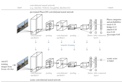
As we have limited training data, we use a transfer learning approach [42] to leverage the knowledge of the pre-trained Places365 CNN, as this CNN already performs well in scene recognition. Figure 5
illustrates the method used for this approach. We fine-tune all the layers of the CNN, trained on the Places365 database, to predict the scenicness of images. We examine the performance of all four different CNN architectures that have been used to train the Places365 CNN: AlexNet [43], Visual Geometry Group (VGG16) [44], GoogleNet [45] and ResNet152 [37]. For all our experiments, we use the deep learning framework Caffe [46]. For AlexNet, VGG16 and GoogleNet, training is performed by stochastic gradient descent (SGD) with mini-batch size 50, a learning rate 0.0001 and momentum 0.9 for 10 000 iterations. For ResNet152, training is performed using a mini-batch size of 10 (due to GPU memory constraints) for 50 000 iterations, to ensure all four networks were exposed to the same amount of images.
6
rsos
.ro
yalsociet
ypublishing
.or
g
R.
Soc
.open
sc
i.
4
:1
70
170
...elastic net coefficients all valley coast mountain snowy lagoon mountain cliff lake natural river glacier waterfall islet mountain path butte snowfield rock arch japanese garden volcano tundra creek cottage castle church ruin ice shelf hayfield pond ski slope formal garden canal natural saturation pasture beach yellow forest path boathouse viaduct lighthouse desert road village arch forest broadleaf vineyard ice floe wave tree farm desert sand rainforest wheat field grotto swamp desert vegetation camping raft tower rugged harbor aqueduct boardwalk natural botanical garden orchard snow pier field road lawn topiary garden swimming forest road badlands marsh blue golf course orange trees rope bridge vegetation mansion field cultivated picnic area oast house brightness foliage running water green
0 0.2 0.4 0.6 −0.2 −0.1 0
construction site hospital parking lot industrial area roof garden excavation playground highway kennel gas station athletic field manufactured home campus amusement park parking garage motel fire station racecourse raceway runway hangar water tower greenhouse general store loading dock street crosswalk junkyard house bridge yard apartment building hunting lodge slum soccer field driveway railroad track residential neighborhood shed bus station park oilrig man made barn airfield dirt soil colour variation pavilion red white no horizon schoolhouse synagogue wind farm brown phone booth grass inn natural light farm corn field driving hiking kasbah open area clouds warmth rice paddy grey positive negative
Figure 2.(Caption opposite.)
well [47]. Further experiments would be required to conclusively state which network might be best suited for prediction of scene aesthetics.
OurScenic-Or-Notdatabase contains only one image per 1 km2grid square, and only in Great Britain.
7
rsos
.ro
yalsociet
ypublishing
.or
g
R.
Soc
.open
sc
i.
4
:1
70
170
...
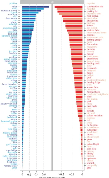
Figure 2.(Opposite.) Elastic net coefficients for all areas in Great Britain. We build an elastic net model to identify features that might be
most relevant for understanding scenicness. We include features related to the colour composition of images such as the percentage of a selection of 11 colours, as well as ‘saturation’ and ‘brightness’ and ‘colour variation’. We also include 102 scene attributes (e.g. ‘natural’, ‘man made’ and ‘open area’) and 205 outdoor place categories (e.g. ‘mountain’, ‘lake natural’, ‘residential neighbourhood’), which have
been extracted using the Places CNN [30,31]. Tables S1 and S2 in the electronic supplementary material list all the scene attributes and
the outdoor place categories that were included in the model. The model accords with intuition, whereby natural features are most associated with greater scenicness, such as ‘Valley’, ‘Coast’ and ‘Mountain’, while man-made features such as ‘Construction Site’ and ‘Industrial Area’ are most associated with lower scenicness. However, man-made features such as ‘Cottage’, ‘Castle’ and ‘Lighthouse’ are
also associated with greater scenicness. In line with Appleton’s prospect–refuge theory [3], we also see features depicted in the results
such as ‘No Horizon’ and ‘Open Areas’, which might reflect preferences shaped by our evolution. We examine this further in the Discussion.
Note that thex-axes for the positive and negative coefficients have different scales.
elastic net coefficients urban built-up
canal natural forest path church cottage castle tower pond river pasture green marsh creek viaduct formal garden orchard boathouse lighthouse forest broadleaf lake natural foliage field road trees mansion village warmth oast house tree farm black inn aqueduct vegetation swamp cemetery hayfield
0 0.05 0.10 0.15 0.20 –0.10 –0.05 0
transporting
excavation parking lot
manufactured home
bus station
construction site
grey
parking garage
athletic field
street
apartment building
crosswalk
loading dock
natural light
white general store
residential neighbourhood
grass
driving campus
man made
kennel
motel
fire station
gas station
playground highway
railroad track
industrial area
colour variation hospital
positive negative
Figure 3.Elastic net coefficients for urban built-up areas in Great Britain. We build an elastic net model to identify features that might be
most relevant for understanding scenicness in built-up urban areas, which might have their own definition of scenicness. We include features related to the colour composition of images such as the percentage of a selection of 11 colours, as well as ‘saturation’ and ‘brightness’ and ‘colour variation’. We also include 102 scene attributes (e.g. ‘natural’, ‘man made’ and ‘open area’) which have been
extracted using the Places205 CNN [32] and 205 outdoor place categories (e.g. ‘mountain’, ‘lake natural’, ‘residential neighbourhood’)
which have been extracted using the Places365 CNN [33]. Tables S1 and S2 in the electronic supplementary material list all the scene
attributes and the outdoor place categories that were included in the model. We do indeed find that the definition of scenicness is different for urban built-up locations. We see that natural features that one might more commonly encounter in urban settings such as ‘Canal Natural’, ‘Pond’ and ‘Trees’ are most associated with greater scenicness. We also see historical buildings such as ‘Church’, ‘Castle’ and ‘Tower’, as well as bridge-like structures such as ‘Aqueduct’ are associated with greater scenicness. Interestingly, in both the model
trained on urban built-up areas (depicted here) and the model trained on all of ourScenic-Or-Notimages (depicted infigure 2), large
flat areas of greenspace such as ‘Grass’ and ‘Athletic Field’ are associated with lower scenicness. Note that thex-axes for the positive and
8
rsos
.ro
yalsociet
ypublishing
.or
g
R.
Soc
.open
sc
i.
4
:1
70
[image:9.522.63.460.52.692.2]170
...
valley
0.15 0.31
0.00 0.46 0.61
(a)
(b)
cottage
0.19 0.38
1.00 0.76
industrial
0.20 0.39
0.00 0.59 0.79
no horizon
0.20 0.40
0.00 0.60 0.80
grass
0.20 0.40
0.00 0.60 0.80
0.00
castle
0.19 0.38
1.00 0.57 0.77
0.00
trees
0.19 0.38
1.00 0.57 0.77
0.00
hospital
0.19 0.38
1.00 0.57 0.77
0.00
0.57
9
rsos
.ro
yalsociet
ypublishing
.or
g
R.
Soc
.open
sc
i.
4
:1
70
[image:10.522.56.461.324.598.2]170
...
Figure 4.(Opposite.) Sample images of features extracted via the Places CNN. For each image, we extract scene attributes and place
categories using the Places CNN [30,31], which assigns a probability score to each attribute. For each attribute, we split the range of
probabilities into five equal intervals, and extract a sample image from each interval. (a) Sample images with features that are most
positively associated with scenicness. Natural features, such as ‘Valley’ and ‘Trees’, are understandably associated with more scenicness. However, we also find that certain types of man-made structures, such as ‘Castle’ and ‘Viaduct’, are positively associated with scenicness.
(b) Sample images with features that are most negatively associated with scenicness. As expected, images that are primarily ‘Industrial’
or contain unsightly man-made objects are not considered as scenic as those without such features. We also find that if a scene has a restricted field of view, such ‘No Horizon’, images are also rated as unscenic. Surprisingly, we find ‘Grass’ is also negatively associated with scenicness. It might be that images that contain the most grass lack other features such as trees or hill contours, resulting in an uninteresting scene. Owing to the different shapes of the photographs, some images have been cropped to aid presentation in this figure.
Full URLs for the original images are provided in the electronic supplementary material. Photographers of ‘Valley’ images:©Alan Stewart,
©Anne Burgess,©Joe Regan,©Chris Wimbush,©Chris Eilbeck. Photographers of ‘Trees’ images:©Alexander P Kapp,©Bob Jenkins,
©Tom Pennington,©Colin Smith,©James Allan. Photographers of ‘Castle’ images:©Gordon Hatton,©Iain Macaulay,©Anne Burgess,
©David Smith,©Ceri Thomas. Photographers of ‘Cottage’ images:©Eirian Evans,©Dennis Thorley,©Jeff Collins,© Colin Grice,
©Robert Edwards. Photographers of ‘Industrial’ images:©John Lucas,©Jonathan Billinger,©Chris Heaton,©M J Richardson,©Oliver
Dixon. Photographers of ‘Hospital’ images:©Richard Webb,©Chris L L,©Colin Bates,©Iain Thompson,©Robin Hall. Photographers
of ‘No Horizon’ images:©Dr Neil Clifton,©Nigel Brown,©Kate Nicol,©Row17,©Oliver Dixon. Photographers of ‘Grass’ images:
©Stephen Pearce,©Row17,©Rob Farrow,©Paul Glazzard,©Mike Quinn. Copyright of the images is retained by the photographers.
Images are licensed for reuse under the Creative Commons Attribution-Share Alike 2.0 Generic License. To view a copy of this licence, visit http://creativecommons.org/licenses/by-sa/2.0/.
Places categories and probabilities tower 0.19 bridge 0.13 church 0.10 river 0.10 skyscraper 0.05 ...
scenic score 4.54463
convolutional neural network
(e.g. AlexNet, VGG16, GoogleNet, ResNet152) output input
pre-trained Places365 convolutional neural network
scenic convolutional neural network 164 937
training images from
Scenic-Or-Not
transfer learning
... ... ...
convolutional and ReLU
pooling convolutional
and ReLU
pooling fully connected
layers
...
flatten
... ...
convolutional and ReLU
pooling convolutional
and ReLU
pooling ... ...
fully connected layers flatten
Figure 5.Using transfer learning to predict scenicness. As CNNs have shown tremendous progress in computer vision tasks [40,41],
we check whether we can use a CNN to predict the scenic ratings of images with a high degree of accuracy. Here, we provide an abstract illustration of the CNN architecture and our approach. As we have limited training data, we use a transfer learning approach
[42] to leverage the knowledge of the Places365 CNN. We modify the final layer of our CNN to predict scenic scores rather than the
probabilities of place categories. We fine-tune all the layers of the CNN, trained on the Places365 database, to predict the scenicness
of images using the four different CNN architectures that have been used to train the Places365 CNN: AlexNet [43], Visual Geometry
Group (VGG16) [44], GoogleNet [45] and ResNet152 [37]. Image©Philip Halling. Copyright of the image is retained by the photographer.
10
rsos
.ro
yalsociet
ypublishing
.or
g
R.
Soc
.open
sc
i.
4
:1
70
170
...
Table 1.Scenic prediction results. We check to what degree we can predict the beauty of scenes for new places for which we do not have
survey or crowdsourced scenicness data. Our first model is an elastic net model to predict the scenicness of images. Our second model is a CNN fine-tuned on the Places365 CNN to predict the scenicness of images. We check the performance on four different CNN architectures
that have been used to train the Places365CNN: AlexNet [43], Visual Geometry Group (VGG16) [44], GoogleNet [45] and ResNet152 [37].
We hold out a 20% test set to check our prediction accuracy. We calculate a performance measure using the Kendall rank correlation between the predicted scenic scores and the actual scenic scores. All four Scenic CNNs outperform the elastic net model in both of our
datasets, with allScenic-Or-Notimages, and also with only Urban Built-upScenic-Or-Notimages. The Scenic CNN trained using the VGG16
CNN architecture delivers the best performance overall.
scenic CNN
elastic net AlexNet VGG16 GoogleNet ResNet152
all 0.544 0.627 0.658 0.653 0.654
. . . .
urban built-up 0.445 0.553 0.590 0.590 0.567
. . . .
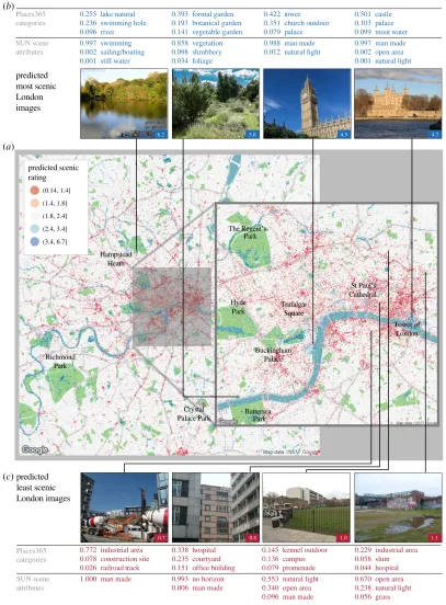
the scenic ratings of 243 339 outdoor London images uploaded toGeograph.We use the Places CNN [32] to determine whether an image has been taken outdoors. The labels of the top five predicted place categories can be used to check if the given image is indoors or outdoors with more than 95% accuracy [32]. With a performance accuracy of 0.658, we find that, in general, our scenic estimates from the CNN accord with what we might expect.Figure 6ademonstrates that parks known for their scenery, such as Hampstead Heath and Richmond Park, have large clusters of scenic imagery. We also see that areas around large bodies of water such as the Thames also seem to contain the most scenic imagery. The most unscenic images seem to be located in the city centre. However, a close-up view reveals clusters of highly scenic imagery in attractive built-up areas, such as Trafalgar Square. An examination of the photos predicted to be scenic indicates that while our Scenic CNN predicts high ratings for images containing primarily natural elements, images of man-made elements, particularly historical architecture around the city, including Big Ben and the Tower of London, are also predicted to be scenic (figure 6b). While our Scenic CNN in general predicts low ratings for images containing primarily man-made features, images containing large areas of drab or unmaintained greenspace and images with a restricted view are also rated as unscenic (figure 6c).
4. Conclusion
We consider whether crowdsourced data generated from over 200 000 images from the existing online gameScenic-Or-Not, combined with the ability to extract hundreds of features from the images using the CNN Places365, might help us understand what beautiful outdoor spaces are composed of. We attempt to find answers to our question that go beyond the simple explanation that ‘what is natural is beautiful’, and explore what features contribute to beauty in urban and built-up settings.
We find, as expected, that natural features, such as ‘Coast’ and ‘Mountain’, are indeed associated with greater scenicness. However, in urban built-up areas, the definition of scenicness varies, and instead we see that natural features such as ‘Pond’, ‘Garden’ and ‘Trees’ are associated with greater scenicness. Surprisingly, we also find that man-made features can also be rated as scenic, in general as well as in urban built-up settings specifically. We find that historical buildings, such as ‘Cottage’ and ‘Castle’, as well as bridge-like structures, such as ‘Viaduct’ and ‘Aqueduct’, are associated with greater scenicness.
What we find to be unscenic might provide the greatest insights. While, as expected, we find that man-made features such as ‘Construction Site’ and ‘Parking Lots’ are associated with lower scenicness, large areas of greenspace such as ‘Grass’ and ‘Athletic Field’ can also lead to lower scenic ratings. Evolution might have conditioned us to dislike certain natural settings if they have attributes that are detrimental to our survival [4]. For example, we seem to dislike certain natural settings if they appear to be drab or neglected [48], or simply uninteresting to explore [9,10]. We also find that ‘No Horizon’ and ‘Open Spaces’ are also associated with lower scenicness. This accords with Jay Appleton’s theory of ‘prospect and refuge’ [3], which suggests that humans have evolved to prefer outdoor spaces where one can easily survey ‘prospects’ and which contain ‘refuge’ where one can easily hide and avoid potential dangers.
11
rsos
.ro
yalsociet
ypublishing
.or
g
R.
Soc
.open
sc
i.
4
:1
70
170
... predicted scenic rating (0.14, 1.4] (1.4, 1.8] (1.8, 2.4] (2.4, 3.4] (3.4, 6.7] Places365 categories SUN scene attributes 5.0 4.5 6.2 4.70.7 0.8 1.1
formal garden botanical garden vegetable garden vegetation shrubbery foliage 0.393 0.193 0.141 0.858 0.098 0.034 industrial area construction site railroad track man made 0.772 0.078 0.026 1.000 hospital courtyard office building no horizon man made 0.338 0.235 0.151 0.993 0.006 industrial area slum hospital open area natural light grass 0.229 0.058 0.044 0.670 0.238 0.056 lake natural swimming hole river swimming sailing/boating still water 0.255 0.236 0.096 0.997 0.002 0.001 tower church outdoor palace man made natural light 0.422 0.351 0.079 0.988 0.012 castle palace moat water man made open area natural light 0.501 0.103 0.099 0.997 0.002 0.001 Places365 categories SUN scene attributes Hampstead Heath Richmond Park Crystal Palace Park The Regent’s Park Hyde Park Buckingham Palace Battersea Park Tower of London Trafalgar Square St Paul’s Cathedral (a)
(b)
(c) predicted most scenic London images predicted least scenic London images 1.0 kennel outdoor campus promenade natural light open area man made 0.145 0.136 0.079 0.553 0.340 0.096
Figure 6.(Caption opposite.)
analysis of the performance of our CNN, we present our predictions for images in London, and find that they are broadly in line with intuition. Our Scenic CNN predicts high ratings for images containing primarily natural elements, such as those located in parks in London known for their attractive scenery, such as Hampstead and Richmond Park, and also predicts high scenic ratings for beautiful buildings, such as the iconic Big Ben and the Tower of London.
12
rsos
.ro
yalsociet
ypublishing
.or
g
R.
Soc
.open
sc
i.
4
:1
70
170
...
Figure 6.(Opposite.) Predictions of scenic ratings for London images. In order to predict the scenic ratings of images for which we do
not already have crowdsourced data, we use a transfer learning approach to leverage the knowledge of the Places365 CNN [24], which
can predict the place category of a scene with a high degree of accuracy. We modify the Places CNN to instead predict the scenicness of
an image. We check the performance on four different CNN architectures that have been used to train the Places365CNN: AlexNet [43],
Visual Geometry Group (VGG16) [44], GoogleNet [45] and ResNet152 [37]. We hold out a 20% test set to check our prediction accuracy. We
calculate a performance measure using the Kendall rank correlation between the predicted scenic scores and the actual scenic scores. The Scenic CNN trained using the VGG16 CNN architecture delivers the best performance with an overall prediction accuracy of 0.658. With our
new Scenic CNN, we predict the scenicness of pictures of London uploaded toGeograph(http://www.geograph.org.uk/), an online project
that collects geographically representative photographs of Great Britain and Ireland. Note that only those categories and features given
a probability of 0.001 or higher have been included in the figure. (a) Examining the estimates of how scenic images around London are,
we immediately notice that parks known for their stunning scenery such as Hampstead Heath and Richmond Park have large clusters of images rated as scenic. The city centre appears to be largely unscenic, although a close-up view reveals clusters of scenic images in
built-up areas. (b) A sample of the top 5% of the photos predicted as scenic indicates that our Scenic CNN mostly predicts high ratings for images
containing primarily natural elements. However, we also see that images containing primarily man-made objects can also be estimated as scenic. Notably, our Scenic CNN has also picked two well-known icons of London—Big Ben and the Tower of London—and rated them as scenic. This is in line with the results of our elastic net analysis, where ‘Tower’ and ‘Castle’ are features that are significantly associated with scenicness. (c) A sample of the bottom 5% of the photos predicted as scenic indicates that our CNN predicts low ratings for images containing primarily man-made features. Images with a restricted view can also be rated as scenic. However, images containing large areas of greenspace also tend to be rated low if they are largely flat and uninteresting or unmaintained. Owing to the different shapes of the photographs, some images have been cropped to aid presentation in this figure. Full URLs for the original images are provided in the
electronic supplementary material. Photographers of scenic images:©Stephen McKay,©Christine Matthews,©Christine Matthews,
©Roger Davies; Photographers of unscenic images:©Stephen Craven,©Robert Lamb,©John Salmon,©Marathon. Copyright of the
images is retained by the photographers. Images are licensed for reuse under the Creative Commons Attribution-Share Alike 2.0 Generic
License. To view a copy of this licence, visithttp://creativecommons.org/licenses/by-sa/2.0/.
In general, our findings offer insights which may help inform how we might design spaces to increase human well-being. It appears that the old adage ‘natural is beautiful’ seems to be incomplete: flat and uninteresting green spaces are not necessarily beautiful, while characterful buildings and stunning architectural features can be. Particularly in urban areas, features such as ponds and trees seem to be important for city beauty, while spaces that feel closed-off or those that are too open and offer no refuge seem to be spaces that we do not rate as beautiful and do not prefer to spend time in. This accords with research that investigates whether our preferences for certain environments might be shaped by evolution, which explains our attraction not only to natural spaces [6,7] but also to ones where we might feel more safe [3] or spaces that are interesting to explore [8–10].
Our findings demonstrate that the availability of large crowdsourced datasets, coupled with recent advances in neural networks, can help us develop a deeper understanding of what environments we might find beautiful. Crucially, such advances can help us develop vital evidence necessary for policymakers, urban planners and architects to make decisions about how to design spaces that will most increase the well-being of their inhabitants.
Data accessibility. This study was a re-analysis of existing data that are publicly available. Data on Scenic-Or-Notratings are openly available at http://scenicornot.datasciencelab.co.uk. We retrieved scenicness ratings by accessing theScenic-Or-Not website on 2 August 2014. TheScenic-Or-Notdataset used in this study is available via the Dryad Digital Repository (http://dx.doi.org/10.5061/dryad.rq4s3) [49]. Geograph images are openly available to download from http://www.geograph.org.uk/. We retrieved images of London fromGeograph on 25 October 2016. The dataset ofGeograph images used infigure 6is available via the Dryad Digital Repository (http://dx.doi.org/10.5061/dryad.rq4s3) [49]. The Places CNNs are openly available to download athttp://places. csail.mit.edu/. The Caffe deep learning framework [46] can be accessed at http://caffe.berkeleyvision.org/. The glmnet package in R was used for the elastic net model implementation [48].
Authors’ contributions.C.I.S., T.P. and H.S.M. designed the study and collected the data; C.I.S. carried out the statistical analyses; C.I.S., T.P. and H.S.M. discussed the analysis and results and contributed to the text of the manuscript. All authors gave final approval for publication.
Competing interests. We declare we have no competing interests.
13
rsos
.ro
yalsociet
ypublishing
.or
g
R.
Soc
.open
sc
i.
4
:1
70
170
...Technology Platform, University of Warwick) and Microsoft Azure (cloud computing resources kindly provided through a Microsoft Azure for Research Award).
References
1. Zukin S. 1995The cultures of cities. Hoboken, NJ: Wiley-Blackwell.
2. Reynolds F. 2015Urbanisation and why good planning matters. London, UK: Oneworld Publications.
3. Appleton J. 1996The experience of landscape. Hoboken, NJ: Wiley-Blackwell.
4. Ulrich RS. 1993 Biophilia, biophobia, and natural landscapes. InThe biophilia hypothesis(eds SR Kellert, EO Wilson), pp. 73–137. Washington, DC: Island Press.
5. Porteous JD. 2013Environmental aesthetics: ideas, politics and planning. Abingdon, UK: Routledge. 6. Orians GH, Heerwagen JH. 1992 Evolved responses
to landscapes. InThe adapted mind: evolutionary psychology and the generation of culture(eds JH Barkow, L Cosmides, J Tooby), pp. 555–579. New York, NY: Oxford University Press.
7. Kellert SR, Wilson EO. 1995The biophilia hypothesis. Washington, DC: Island Press.
8. Ulrich RS. 1983Aesthetic and affective response to natural environment, pp. 85–125. Boston, MA: Springer.
9. Kaplan S, Kaplan R, Wendt JS. 1972 Rated preference and complexity for natural and urban visual material.Percept. Psychophys.12, 354–356. (doi:10.3758/BF03207221)
10. Kaplan R, Kaplan S. 1989The experience of nature: a psychological perspective. Cambridge, UK: Cambridge University Press.
11. Küller R. 1972A semantic model for describing perceived environment. Stockholm, Sweden: National Swedish Institute for Building Research.
12. Ball K, Bauman A, Leslie E, Owen N. 2001 Perceived environmental aesthetics and convenience and company are associated with walking for exercise among Australian adults.Prev. Med.33, 434–440. (doi:10.1006/pmed.2001.0912)
13. Giles-Corti B, Broomhall MH, Knuiman M, Collins C, Douglas K, Ng K, Lange A, Donovan RJ. 2005 Increasing walking: how important is distance to, attractiveness, and size of public open space?Am. J. Prev. Med.28, 169–176. (doi:10.1016/j.amepre. 2004.10.018)
14. Arthur LM. 1977 Predicting scenic beauty of forest environments: some empirical tests.For. Sci.23, 151–160.
15. Real E, Arce C, Manuel Sabucedo J. 2000 Classification of landscapes using quantitative and categorical data, and prediction of their scenic beauty in North-Western Spain.J. Environ. Psychol.20, 355–373. (doi:10.1006/jevp.2000.0184) 16. Arriaza M, Canas-Ortega JF, Canas-Madueno JA,
Ruiz-Aviles P. 2004 Assessing the visual quality of rural landscapes.Landsc. Urban Plan.69, 115–125. (doi:10.1016/j.landurbplan.2003.10.029) 17. Joye Y. 2007 Architectural lessons from
environmental psychology: the case of biophilic architecture.Rev. Gen. Psychol.11, 305–328. (doi:10.1037/1089-2680.11.4.305)
18. Stamps AE. 2002 Fractals, skylines, nature and beauty.Landsc. Urban Plan.60, 163–184. (doi:10.1016/S0169-2046(02)00054-3) 19. Seresinhe CI, Preis T, Moat HS. 2015 Quantifying the
impact of scenic environments on health.Sci. Rep.5, 16899. (doi:10.1038/srep16899)
20. Salesses P, Schechtner K, Hidalgo CA. 2013 The collaborative image of the city: mapping the inequality of urban perception.PLoS ONE8, e68400. (doi:10.1371/journal.pone.0068400)
21. Quercia D. 2013 Urban*: crowdsourcing for the good of London. InProc. of the 22nd Int. World Wide Web Conf.,Rio de Janeiro, Brazil,13–17 May 2013, pp. 591–592.
22. Olshausen BA, Field DJ. 1996 Emergence of simple-cell receptive field properties by learning a sparse code for natural images.Nature381, 607–609. (doi:10.1038/381607a0)
23. Graham DJ, Hughes JM, Leder H, Rockmore DN. 2012 Statistics, vision, and the analysis of artistic style.
WIREs Comp. Stat.4, 115–123. (doi:10.1002/wics. 197)
24. Csurka G, Dance C, Fan L, Willamowski J, Bray C. 2004 Visual categorization with bags of keypoints. InWorkshop on Statistical Learning in Computer Vision,ECCV, Prague,Czech Republic,15 May 2004.
25. Quercia D, O’Hare NK, Cramer H. 2014 Aesthetic capital: what makes London look beautiful, quiet, and happy. InProc. of the 17th ACM conf. on Computer Supported Cooperative Work & Social Computing,Baltimore, MD,15–19 February 2014, pp. 945–955.
26. Donahue J, Jia Y, Vinyals O, Hoffman J, Zhang N, Tzeng E, Darrell T. 2014 DeCAF: a deep convolutional activation feature for generic visual recognition. In
Int. Conf. in Machine Learning,Beijing, China,21–16 June 2014, vol. 32, pp. 647–655.
27. Sharif Razavian A, Azizpour H, Sullivan J, Carlsson S. 2014 CNN features off-the-shelf: an astounding baseline for recognition. InProc. of the IEEE Conf. on Computer Vision and Pattern Recognition Workshops,
Columbus, OH,23–28 June 2014, pp. 806–813. 28. Tan Y, Tang P, Zhou Y, Luo W, Kang Y, Li G. 2017
Photograph aesthetical evaluation and classification with deep convolutional neural networks.Neurocomputing228, 165–175. (doi:10.1016/j.neucom.2016.08.098) 29. Lu X, Lin Z, Jin H, Yang J, Wang JZ. 2015 Rating
image aesthetics using deep learning.IEEE Trans. Multimedia17, 2021–2034. (doi:10.1109/TMM.2015. 2477040)
30. De Nadai M, Vieriu RL, Zen G, Dragicevic S, Naik N, Caraviello M, Hidalgo CA, Sebe N, Lepri B. 2016 Are safer looking neighborhoods more lively? A multimodal investigation into urban life. InProc. of the 2016 ACM on Multimedia Conf.,Amsterdam, The Netherlands,15–19 October, pp. 1127–1135. 31. Dubey A, Naik N, Parikh D, Raskar R, Hidalgo CA.
2016 Deep learning the city: quantifying urban perception at a global scale. InEuropean Conf. on
Computer Vision, Amsterdam,The Netherlands,8–16 October 2016, pp. 196–212.
32. Zhou B, Lapedriza A, Xiao J, Torralba A, Oliva A. 2014 Learning deep features for scene recognition using places database. InAdvances in Neural Information Processing Systems 27,Montreal, Canada,8–13 December 2014, pp. 487–495.
33. Zhou B, Khosla A, Lapedriza A, Torralba A, Oliva A. 2016 Places: an image database for deep scene understanding. (https://arxiv.org/abs/1610.02055). 34. Seresinhe CI, Moat HS, Preis T. In press. Quantifying scenic areas using crowdsourced data.Environ. Plan. B: Urban Analytics and City Science.
(doi:10.1177/0265813516687302)
35. Stadler B, Purves R, Tomko M. 2011 Exploring the relationship between Land Cover and subjective evaluation of scenic beauty through user generated content. InProc. of the 25th International Cartographic Conference,Paris, France,July 2011.
36. Patterson G, Xu C, Su H, Hays J. 2014 The SUN attribute database: beyond categories for deeper scene understanding.Int. J. Comput. Vision.108, 59–81. (doi:10.1007/s11263-013-0695-z) 37. He K, Zhang X, Ren S, Sun J. 2016 Deep residual
learning for image recognition. InProc. of the IEEE Conf. on Computer Vision and Pattern Recognition,
Seattle, WA,27–30 June 2016, pp. 770–778. 38. Office for National Statistics. 2013The 2011
rural–urban classification for small area geographies.London, UK: Office for National Statistics Publications.
39. Scottish Government. 20122011–2012 urban rural classification. Edinburgh, UK: Scottish Government. 40. Morton D, Rowland C, Wood C, Meek L, Marston C,
Smith G, Wadsworth R, Simpson, I. 2014Land cover map 2007(vector, GB), v. 1.2. Wallingford, UK: NERC Environmental Information Data Centre. 41. Zou H, Hastie T. 2005 Regularization and variable
selection via the elastic net.J. R. Stat. Soc. B.
67, 301–320. (doi:10.1111/j.1467-9868.2005.00503.x) 42. Pan SJ, Yang Q. 2010 A survey on transfer learning.
IEEE Trans. Knowl. Data Eng.22, 1345–1359. (doi:10.1109/TKDE.2009.191)
43. Alex K, Sutskever I, Hinton GE. 2012 ImageNet classification with deep convolutional neural. In
Advances in Neural Information Processing Systems 25,Lake Tahoe, NV,3–8 December 2012, pp. 1097–1105.
44. Simonyan K, Zisserman A. 2014 Very deep convolutional networks for large-scale image recognition. InProc. Int. Conf. on Learning Representations, Banff,Canada,14–16 April 2014. 45. Szegedy C, Liu W, Jia Y, Sermanet P, Reed S,
Anguelov D, Erhan D, Vanhoucke V, Rabinovich A. 2015 Going deeper with convolutions. In2015 IEEE Conf. on Computer Vision and Pattern Recognition,
Boston, MA,7–12 June 2015, pp. 1–9. 46. Jia Y, Shelhamer E, Donahue J, Karayev S, Long J,
14
rsos
.ro
yalsociet
ypublishing
.or
g
R.
Soc
.open
sc
i.
4
:1
70
170
...
embedding. InProc. of the 22nd ACM Int. Conf. on Multimedia,Orlando, FL,3–7 November 2014, pp. 675–678.
47. Kabkab M, Hand E, Chellappa R. 2016. On the size of convolutional neural networks and generalization performance. InProceedings from the 23rd Int. Conf.
on Pattern Recognition (ICPR),Cancun, Mexico,4–8 December 2016, pp. 3572–3577.
48. Akbar KF, Hale WHG, Headley AD. 2003 Assessment of scenic beauty of the roadside vegetation in northern England.Landsc. Urban Plan.63, 139–144. (doi:10.1016/S0169-2046(02)00185-8)
49. Seresinhe C, Preis TG, Moat H. 2017 Data from: Using deep learning to quantify the beauty of outdoor places. Dryad Digital Repository.