http://www.sciencepublishinggroup.com/j/ijdsa doi: 10.11648/j.ijdsa.20190505.15
ISSN: 2575-1883 (Print); ISSN: 2575-1891 (Online)
Bayesian Finite Mixture Negative Binomial Model for
Over-dispersed Count Data with Application to DMFT Index
Data
Kipngetich Gideon, Anthony Wanjoya, Samuel Mwalili
Department of Statistics and Actuarial Science, Jomo Kenyatta University of Agriculture and Technology, Nairobi, Kenya
Email address:
To cite this article:
Kipngetich Gideon, Anthony Wanjoya, Samuel Mwalili. Bayesian Finite Mixture Negative Binomial Model for Over-dispersed Count Data with Application to DMFT Index Data. International Journal of Data Science and Analysis. Vol. 5, No. 5, 2019, pp. 104-110.
doi: 10.11648/j.ijdsa.20190505.15
Received: October 8, 2019; Accepted: October 23, 2019; Published: October 30, 2019
Abstract:
To establish viable statistical model for modelling and analyzing DMFT index data which is important in oral health studies, difficulty arise when DMFT index data is characterized by over-dispersion. Over-dispersion caused by unobserved heterogeneity in the data pose a problem in fitting more common models to this data. and failure to account on such heterogeneity in the model can undermine the validity of the empirical results. The limitations of other count data models to account for overdispersion in DMFT index data due to existence of heterogeneity in the data, this paper formulated alternative model that captures heterogeneity in the data, that is Bayesian Finite mixture negative binomial regression model and the model applied to simulated overdispersed count data to determine the exact number of negative binomial components to be mixed and finally apply the model to DMFT index data. Bayesian finite mixture Negative Binomial (BFMNB-3) regression model is useful since the data were collected from heterogenous population. simulation results shows that 3-component Bayesian finite mixture of NB regression model converges and was quite enough to model the overdispersed simulated count data, applying BFMNB-3 model to DMFT index data, the model capability to capture heterogeneity in the data identifies that the methods; all the treatment (all methods together), mouth wash with 0.2% sodium fluoride and Oral hygiene were the best methods in preventing tooth decay in children in Belo Horizonte (Brazil) aged seven years this shows that BFMNB-3 performs better than BNB model were due to heterogeneity present in methods it only identifies methods; all the treatment (all methods together) and mouth wash with 0.2% sodium fluoride to be the best methods for preventing tooth decay for children in Belo Horizonte (Brazil) aged seven while this two methods were not the only significant methods, therefore from results there is complete superiority of BFMNB-3 over BNB model. R statistical software was used to accomplish the objectives of this paper.Keywords:
BFMNB-3 Model, DMFT Index Data, BNB1. Introduction
Count data is encountered in many areas of research including social sciences, transport, economic and health, count data includes; the number of accidents in a specified period of time, number of epileptic seizures in a week, number of insurance claims paid by Insurance company in a year, number of domestic violence and number of defective items in a batch of manufactured items. This count data has different forms that is, count data with excess number of zeros, count data with large observations and count data
underlying assumption of equidispersion limits its use in many real-world applications where over and under-dispersed count data is encountered [2] overdispersion and under dispersion can lead to inconsistent standard errors of parameter estimates when Poisson model is used [5-6], due to existence of overdispersion mainly due to generation of excess zero’s. Negative Binomial, in this distribution the distribution’s parameter is itself considered a random variable and variation of this parameter can account for variance of the data that is higher than the mean, this serves as a good alternative to handle overdispersed count data [7], zero-inflated double Poisson model could be a viable alternative to the joint modeling of excess of zeros and over-dispersion (or under-over-dispersion). Over and Under-dispersed count data is conveniently model by Conway-Maxwell regression model [8, 9] and Double Poisson regression model [10-11]. and have been found to be very flexible to handle overdispersed count data [11-14] model discrete count using Bayesian framework in Win Bugs [15] but parameter estimation still remain to be complex and difficult. Although Conway-Maxwell-Poisson distribution could be a feasible alternative to model over-dispersion and under-dispersion count data, it is observed that it requires a lot of computation for parameter estimation [16] also perform less compared to Double Poisson where there is high sample mean for all types of dispersion [17], major challenge with Double Poisson distribution is, results are not exact since the normalizing constant has no closed form solution [4]. The study proposes Bayesian Finite mixture model to fit over-dispersed count data because when posterior distribution for the unknown parameters are given, Bayesian method provide valid inference without relying on the asymptotic normality and this is important when the sample size is small. In the study, BFMNB-k was formulated its performance accessed by fitting to over-dispersed Simulated count data and finally apply BFMNB – 3 model to DMFT index data.
2. Literature Review
Bayesian analysis represent prior uncertainty about model parameters having probability distribution and updating prior uncertainty with current data to induce posterior probability distribution for the parameter with less uncertainty. In Bayesian analysis, model parameters are considered random quantities, whereas the data having been already observed are considered fixed quantities. The Bayesian approach provides a fairly explicit solution to common problems of statistical inference, new problems of high-dimensional data analysis that are coming up because of emergence of high-dimensional data sets, and complex decision problems of real life [18].
Models for Count data discussed in this paper, Poisson Regression Model
Poisson has been used as basic model in modeling count data [19] it models equi-dispersed count data that is;
Ε | = | = ( )
but this model fails when we have over-dispersed data. The model is represented as,
∽ ( ) where = ( )
In real life situations count data exhibit overdispersion and the assumptions of equality of mean and variance in Poisson (restrictiveness) fails due to heterogeneity (difference between individuals) and contagion (dependence between the occurrence of events) [17].
[4] To model overdispersed count data, Poisson regression can be modified such that,
∽ ( ) where = ( )
is nonnegative multiplicative random effect term to model individual heterogeneity, and taking total expectation
Ε | = ( ) Ε ( )
Var | = Ε | + Ε Ε |
Therefore, variance is greater than mean and the model can be used now to model overdispersed count data.
Negative Binomial
Negative Binomial have been considered to out-perform Poisson regression model in modeling overdispersed count data [5], it is obtain by placing gamma prior in the nonnegative multiplicative random effect term in Poisson regression model,
∽ !","% = 1 Γ(") "& &() &*+
Where , = 1 and = "() .
Factoring out in Poisson regression we obtain negative binomial parameterized by mean - = exp ( ) and inverse dispersion parameter 1 = )& given by,
2( ) = Γ(3Γ(3 − 1) 5()+ ) 3()3()+ - 67
89
(3()-+ - ):+
And mean Variance is given by;
Ε | = ( )
Var | = Ε | + 3Ε |
Bayesian Poisson Regression Model The model is given by,
∽ ( ) log( ) = >
log( ) = > for i = 1,2, …, n
− regression parameters
> − vector of covariates
(?|> , ) = ( )
Placing prior distributions in the regression parameters where @(. ) induce a prior distribution, that is @( ) =
B (0, D = B) n is the sample size.
Prior distribution and likelihood function define the posterior distribution of the regression parameters (Bayes’ theorem). Samples from the posterior distribution is obtained in PROC MCMC.
To access the goodness of fit
EF= G ? − Ε (?)(?)
H
I)
3. Methodology
Bayesian Finite Mixture Negative Binomial Regression Model [20] Due to heterogeneity (difference between individual) and contagion (dependence between the occurrence of events) count data in real life are usually overdispersed (Variance is greater than the mean).
The random vector ? = ( ), … , K)′ is said to arise from a finite mixture distribution if the probability density function
( ) has the form,
( |Θ) = N)2)( |O)) + … + N&2&( |O&)
Where, Θ = (O), … , O&) vector of all unknown parameters and N ′ are mixing proportions whose elements are restricted as positive and sum to unity.
A single density 2&(. |O&) is component distribution for component " and is assume to arise from the same distribution
The marginal distribution of the mixture is given by;
( | , Θ) = G N&
P
&I)
QRS-,&, T&U
= G N& Γ( + 1)ΓTΓ( + T&) & (
-,&
-,&+ T&)
:+( T&
-,&+ T&) VW
P
&I)
X Y(- ) =
,( | , O) = G -,&N&
P
&I)
( | , Θ) = ,( | , O) + ZG N&-,&!1 + T1
&% P
&I)
[
− ,( | , O)
-,& is the mean, Θ vector of unknown parameters and T& dispersion parameters and goes to infinity in each component.
The variance of is always greater than the mean even if all the components have the same mean. K is sequentially increased until both AIC and BIC value reach their optimal values.
The unobserved random variable variables \ are
independently and identically multinomial with probabilities
w.
(\ |N) = ] N&^+,W
P
&I)
(\ |N) is the likelihood of observing the component
membership vector \ for each site , given the component proportions N. likelihood for site ;
( , \ | , Θ) = ( |\ , , Θ) (\ | , Θ)
= ] ( | , &
P
&I)
, T&) ^+,WN&^+,&
( | , &, T&) − X function of the NB model for "_`
component, likelihood function over all sites;
( , \|Θ, ) = ] ] (
K
I) P
&I)
| , &, T&)^+,WN&^+,W
= ] ] (
K
I) P
&I)
| , &, T&) ^+,W ] N&HW &
&I)
B&= ∑ \KI) ,& number of observations allocated to component ".
posterior distribution given by,
@(b, Θ| , ) ∝ (b, Θ| , >)@(Θ)
Where @(Θ) is the prior for all the parameters and > is the matrix covariates for all sites, [21] Finite mixture allow for additional heterogeneity within components not captured by explanatory variables.
The prior distributions are;
For the unknown regression coefficients d, @( ) =
e QFf)( g, g) ∝ exp −)( &− g)h g()( &− g)
For dispersion parameter is given by;
@(T&) ( , i) ∝ T&j()exp (−iT&)
And prior distribution for weights is given by; @(N) =
k lℎn o( H, … , H) ∝ N&pq()
Dirichlet is uniform when H= 1
The conditional distribution is given by; For the unknown regression coefficients
@S &rΘsW, b, >, U
∝ ] ] (
K
I) P
&I)
| , &, T&) ^+,W
exp −12 ( &− ig)′ g()( &− ig)
For the dispersion parameter T&
∝ ] ]
P
I) K
&I)
| , ^+,W T&j()exp 4iT&
For weights N&
@ N|\ k lmn o
H ), … , H & u ] v&pqfwW() P
&I)
For \ is a multinomial distribution given by;
@S\,&rΘ, > , U
exno B 1, r S\,)rΘ, > , U, … , Sb,&rΘ, > , Ur
4. Data Description
DMFT index data was from the Belo Horizonte Caries Prevention (BELCAP) study. The data was collected from children in Belo Horizonte (Brazil) aged 7 years at the start of the study. determining which method was the best for preventing tooth decay, six treatments were randomized to six separate treatment groups. Only eight deciduous molars were considered, the lowest value was 0, highest was 8. Main reasons for using this dataset; the data is relatively good quality and has been used in various study purposes and the data shows existence of heterogeneity of the several different sub-populations. Data has two sub-population i.e. End (Number of decayed, missing or filled teeth at the end of the study), begin (Number of decayed, missing or filled teeth at the beginning of the study) and covariates (Gender-(male and female), Ethnic (with levels brown, white and black), Treatment (with levels control-Control group, educ-Oral health education, enrich- Enrichment of the school diet with rice bran, rinse-Mouthwash with 0.2% sodium fluoride (NaF) solution, hygiene-Oral hygiene and all-All four methods together).
5. Empirical Results
i) Results from simulation
Sample size of N=1000 was used to generate the data that was used to select the most viable model of Bayesian finite mixture negative binomial. The number of components for mixture was determined and was found to be 3 since the model converge only when 3 components were mixed.
Table 1. Goodness of fit.
number of components (k) AIC BIC
K = 1 2686.13 2707.203 K = 2 1920.231 1966.592 K = 3 1918.456 1939.529
Table 1 show the information criterion at each of components, comparing the BIC for component 1-3 the BIC for model with component 1 was 2707.203 which is very large, for component 1 and 2 although there values are close the BIC for component 3 (1939.529) is smaller compared to BIC for component 2 (1966.592) therefore the model where 3 components of Negative Binomial were mixed is the best to fit the data and research concludes that with 3 components mixed the model provides best fit to overdispersed data.
The output was also visualized using figure 1.
Figure 1. Goodness of fit graph.
Checking for overdispersion in the simulated count data, figure 2 show that there is skeweness to the right this displays presence of over-dispersion also displays the high poroportion of zero’s and that justifies over-dispersion in the data, the summary statistics [M (SD) = 3.15 (5.66)] showed that the mean was 3.15 and the variance was 32.0356 implying that variance is greater than the mean a characteristic present in any overdispersed data.
Figure 2. Histogram for simulated counts from BFMNB-3.
Table 2. BFMNB-3 True and Estimated parameter values.
Model parameters
True Values BFMNB – 3 Values
Component 1 Component 2 Component 3 Component 1 Component 2 Component 3
),&^ 0.0 -0.5 0.5 -0.3178 0.525 0.343
,&
^ 2.0 0.5 -0.5 -0.510 0.123 0.464
z,&^ -0.5 0.5 2.0 -0.510 1.112 0.465
T&^ 5 10 15 4.824 9.112 14
Table 2 displays the parameter values and it is observed that the true and the estimated parameter values have no much difference and therefore they are unbiased for instance True value z,&^ for component one is -0.5 and the value for component one for BFMNB-3 is -0.510 considering also the dispersion parameter T&^ the true values for components 1-3 are 5, 10 and 15 and for BFMNB-3 are 4.824, 9.112 and 14
this values are closer to each other implying less deviation from each other, the same property is also observed in the assignment of weights N& where the weights for component 1-3 were 0.333, 0.333 and 0.333 and the weights assigned to components of BFMNB-3 were 0.324, 0.326 and 0.350.
ii) Applying BFMNB – 3 Model to data (DMFT index data)
Table 3. Summary Statistics for testing over-dispersion in data.
Variables
Y (End) Control all Rinse hygiene enrich education
Mean 1.854454 2.35 1.31 1.65 1.80 2.15 1.86
Variance 2.905925 3.3125 2.2201 2.7889 3.24 2.9584 2.25
Checking for overdispersion in DMFT index data, In Table 3 it was found that the hypothesis {g: u= 0 for no over-dispersion was rejected u= 0.1044174 which is not equal to zero therefore there is over-dispersion in the data. Z-score test had a t-probability of 2e−16 which is less than 0.0005, Z test also evaluate that the data are negative binomial and therefore it suggests that real over-dispersion exists in the data also the existence of overdispersion was also seen in figure 3 were the graph is skewed to the right.
Figure 3. Histogram for DMFT index data.
Figure 4. Goodness of fit of the model to DMFT index data.
Figure 4 show the goodness of fit of BFMNB – 3 model to DMFT index data, from Table 4 the BIC and AIC were significantly smaller for component 3, comparing the model with two components mixed the BIC was 2898.982 and the model with three components mixed had BIC of 2885.572 and although this values were close, they are significantly
different to guarantee the choice of model with three components mixed together. therefore BFMNB-3 model fits DMFT index data well.
Figure 5. Trace plot and Posterior Distribution density.
Table 4. BFMNB-3 Goodness of fit to DMFT index data.
number of components (k) AIC BIC
K = 1 2956.092 2998.22 K = 2 2838.081 2898.932 K = 3 2834.083 2885.572
Figure 5 shows the convergence of the model by trace plot fitted to DMFT index data it was observed that the model converges after 2000 iterations, posterior distributions of the model is bell and monomodal shape of marginal posterior distribution close to a normal distribution although there is evidence of dispersion on the right-hand side of the plot.
Table 5. Coefficient Estimates and Bayes Factors for Model Parameters.
Parameter Estimate Bayes Factor
Figure 6. Posterior and prior Density plots.
Table 5 shows that the parameters for the methods; all methods together, mouth wash with 0.2% sodium fluoride and Oral hygiene had Bayes factor of 18.69, 0.56 and 0.25 respectively all greater than the standard value 0.1 and that all this parameters were significant therefore the methods; all the treatment (all methods together), mouth wash with 0.2% sodium fluoride and Oral hygiene were the best methods in preventing tooth decay in children in Belo Horizonte (Brazil) aged seven years. Table 5 also report the BIC of 2885.572 this value defines the goodness of fit of the BFMNB-3 to DMFT index data the value is lower compared to the BIC (2898.932) for BFMNB-2 therefore BFMNB-3 best fit the data.
From figure 6 the posterior distribution for all the variables are almost the same this is due to the assumption of conjugate priors for the model parameters this is also clear on the density of prior which is same for all the variables.
ii) Applying Bayesian Negative Binomial (BNB) Model to data (DMFT index data)
Applying BNB to DMFT index data it was observed that
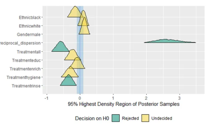
the parameters for methods; all the treatment (all methods together) and mouth wash with 0.2% sodium fluoride were the best method for preventing tooth decay for children in Belo Horizonte (Brazil) aged seven this is explained by low proportions inside ROPE i.e. the closer to zero the better and null hypothesis should be rejected therefore the parameters are significant from Table 6. The same results were also seen in figure 7 where the light blue color defines the most significant parameters.
Table 6. Test for Practical Equivalence (ROPE: [-0.10 0.10]).
Parameter |} inside ROPE 95% HDI
Gender male Undecided 0.34% [-0.01 0.26] Ethnic white Undecided 0.54% [-0.05 0.24] Ethnic black Undecided 0.31% [-0.39 0.06] Treatment education Undecided 0.11% [-0.47 -0.00] Treatment all Rejected 0.00% [-0.83 -0.35] Treatment enrich Undecided 0.51% [-0.32 0.13] Treatment rinse Rejected 0.00% [-0.57 -0.13] Treatment hygiene Undecided 0.02% [-0.55 -0.07] (Intercept) Rejected 0.00% [0.58 0.96] reciprocal-dispersion Rejected 0.00% [1.93 3.46]
Bayesian Negative Binomial for differential expression with confounding factors [22] concluded that BNB is capable of handling and tracking complex experiments involving multiple factors and multi-variate dependence structure, despite this incredible performance of BNB it was observed from the results that it is less capable to capture heterogeneity and uncertainty in the variables under study therefore BFMNB-3 outperforms (since BFMNB-3 was able to identify the 3 components being the best methods to prevent tooth decay) BNB and the research concludes that BFMNB-3 is the most viable model to analyze the DMFT index data.
6. Conclusion
To formulate and apply BFMNB-3 to DMFT index data was the main objective of this paper. The findings of the study were BFMNB-3 model deemed to be the best model in modelling overdispersed data with sub-populations characterized with heterogeneity also the model can handle uncertainty in the data (DMFT index data) it was clearly seen that the model has lower BIC (2885.572). the plots (figures 3 and 5) showed that the model can be used to better reveal the source of dispersion observed in DMFT index data (where treatment was found to be the source of Over-dispersion), The model being capable to capture heterogeneity it was found that the methods; all the treatment (all methods together), mouth wash with 0.2% sodium fluoride and Oral hygiene were the best methods in preventing tooth decay in children in Belo Horizonte (Brazil) aged seven years this shows that BFMNB-3 performs better than BNB model were due to heterogeneity present in methods it was only able to only identify methods; all the treatment (all methods together) and mouth wash with 0.2% sodium fluoride to be the best methods for preventing tooth decay for children in Belo Horizonte (Brazil) aged seven and indeed this two methods were not the only best methods, therefore from results there is complete superiority of BFMNB-3 over BNB model.
References
[1] A. J. Dobson, “An introduction to generalized linear models.” Chapman & Hall/CRC, 2001.
[2] K. F. Sellers and G. Shmueli, “Data dispersion: now you see it… now you don’t,” Commun. Stat. Methods, vol. 42, no. 17, pp. 3134–3147, 2013.
[3] N. C. Pradhan and P. Leung, “A Poisson and negative binomial regression model of sea turtle interactions in Hawaii’s longline fishery,” Fish. Res., vol. 78, no. 2–3, pp. 309–322, 2006.
[4] R. Winkelmann, Econometric analysis of count data. Springer Science & Business Media, 2008.
[5] J. M. Hilbe, Modeling count data. Springer, 2011.
[6] E. S. Park and D. Lord, “Multivariate Poisson-lognormal models for jointly modeling crash frequency by severity,” Transp. Res. Rec., vol. 2019, no. 1, pp. 1–6, 2007.
[7] E. Hauer, Observational before/after studies in road safety. Estimating the effect of highway and traffic engineering measures on road safety. 1997.
[8] J. B. Kadane, G. Shmueli, T. P. Minka, S. Borle, P. Boatwright, and others, “Conjugate analysis of the Conway-Maxwell-Poisson distribution,” Bayesian Anal., vol. 1, no. 2, pp. 363–374, 2006.
[9] G. Shmueli, T. P. Minka, J. B. Kadane, S. Borle, and P. Boatwright, “A useful distribution for fitting discrete data: revival of the Conway--Maxwell--Poisson distribution,” J. R. Stat. Soc. Ser. C (Applied Stat., vol. 54, no. 1, pp. 127–142, 2005.
[10] H. Madsen and P. Thyregod, Introduction to general and generalized linear models. CRC Press, 2010.
[11] Y. Lee, J. A. Nelder, and Y. Pawitan, Generalized linear models with random effects: unified analysis via H-likelihood. Chapman and Hall/CRC, 2018.
[12] D. Lord, S. D. Guikema, and S. R. Geedipally, “Application of the Conway--Maxwell--Poisson generalized linear model for analyzing motor vehicle crashes,” Accid. Anal. Prev., vol. 40, no. 3, pp. 1123–1134, 2008.
[13] K. F. Sellers, S. Borle, and G. Shmueli, “The COM-Poisson model for count data: a survey of methods and applications,” Appl. Stoch. Model. Bus. Ind., vol. 28, no. 2, pp. 104–116, 2012.
[14] S. D. Guikema and J. P. Coffelt, “Modeling count data in risk analysis and reliability engineering,” in Handbook of performability engineering, Springer, 2008, pp. 579–594. [15] D. Spiegelhalter, A. Thomas, N. Best, and D. Lunn,
“WinBUGS user manual.” version, 2003.
[16] Y. Zou, S. R. Geedipally, and D. Lord, “Evaluating the double Poisson generalized linear model,” Accid. Anal. Prev., vol. 59, pp. 497–505, 2013.
[17] Y. Zou, D. Lord, and S. R. Geedipally, “Over-and Under-Dispersed Crash Data: Comparing the Conway-Maxwell-Poisson and Double-Conway-Maxwell-Poisson Distributions,” Texas A & M University, 2012.
[18] J. K. Ghosh, M. Delampady, and T. Samanta, An introduction to Bayesian analysis: theory and methods. Springer Science & Business Media, 2007.
[19] A. C. Cameron and P. K. Trivedi, Regression analysis of count data, vol. 53. Cambridge university press, 2013.
[20] M. Zhou and L. Carin, “Negative binomial process count and mixture modeling,” IEEE Trans. Pattern Anal. Mach. Intell., vol. 37, no. 2, pp. 307–320, 2015.
[21] B.-J. Park, D. Lord, and J. D. Hart, “Bias properties of Bayesian statistics in finite mixture of negative binomial regression models in crash data analysis,” Accid. Anal. Prev., vol. 42, no. 2, pp. 741–749, 2010.