The impact of prior use on the further diffusion of new process
technology
Paul Stoneman*
Warwick Business School, University of Warwick, Coventry, CV4 7AL, UK
This paper contributes to our understanding as to how the extent of prior use of a new technology may impact upon current additions to use. The paper is innovative first in placing emphasis upon intra firm aspects of the diffusion process and secondly by integrating rivalry and spill-over effects (such as early mover advantages, learning by doing, network externalities and learning) in a unified theoretic framework.
Keywords: Diffusion; strategic behaviour; spillovers; bandwagons.
JEL Classification: 03
1. Introduction1
In his career Peter Swann has made many varied and important contributions to our knowledge of the process of technological change. I have chosen to concentrate in this paper upon just one of the areas in which he has made his mark, namely the study of diffusion. In particular it is with process (rather than product2) innovation with which the paper is concerned and the main theme of the paper comes from the quote below, which I have adapted from Peter’s typically very accessible recent book.
“Strategic interaction between players may be an important factor in explaining the rate of diffusion. For example, some adoption decisions may be driven by a desire to forge ahead of competitors in order to achieve a cost, quality or performance advantage. Equally, some adoption decisions may be driven by a need to catch up with competitors and thus to make good a cost, quality or performance disadvantage. ...Or alternatively, the existence of a large installed base is often a powerful signal to some buyers that this technology is no longer the risky prospect that it appeared at first. This feature makes for a very powerful and rapid diffusion process which is sometimes described as a
bandwagon.” (adapted from Swann 2010)
There is a now a considerable literature on technological diffusion (see for example Stoneman 2002) but this quote embodies two main themes that are basic to our
understanding of that process: firstly that rivalry, or strategic interaction, may play a role in the process, and secondly, that there may be various spill over effects from usage, either from one firm to another or from one time to another, that also have an impact. Implicitly, the quote argues that in a context of rivalry, prior use of new technology may impact either positively or negatively upon additions to use, whereas spill-over effects may cause prior use to impact positively upon additions to use. To clarify terminology, we will follow previous practice and consider that if prior use impacts positively on
1 This paper is a revised version of a paper presented at a Conference in Honour of Peter Swann O.B.E.
held at the University of Nottingham, September 15th – 16th 2011. An antecedent of the work was presented at the SPRU 40th Anniversary Conference on the Future of Science ,Technology and Innovation Policy, Linking Research and Practice, 11th – 13th September 2006, Brighton. I would like to thank two anonymous referees of this journal for their comments although all errors that remain are the responsibility of the author alone.
2 One of the referees has suggested that the arguments in this paper can be extended to incorporate product
current use then a bandwagon exists. If there is no impact from prior use or the impact is negative than we will consider that a bandwagon does not exist. A particular aim of this paper is to look again at rivalry and spillovers in order to attempt to add to our
understanding of whether bandwagons thus defined may be expected. In doing so however we are innovative in two ways, relative to the existing literature.
First one may note that the existing literatures (see Stoneman 2002 and Geroski 2000) upon strategic behaviour and spill over or bandwagons have tended to develop separately. The extant literature looking at diffusion from a strategic viewpoint e.g. Fudenberg and Tirole (1985) and Reinganum3 (1981), does not tend to encompass issues that might be considered as at the heart of the explanation for bandwagons (i.e. spillover effects). Much of the existing literature that predicts bandwagons however (see, for example, Mansfield 1968, on epidemic learning and the evolutionary approach as presented by Metcalfe 1995) has generally developed outside the remit of models that look at strategic behaviour. Thus, a first innovation in this paper is an attempt to integrate the two approaches by building and exploring the predictions of models in which spill over effects are present but are contained within a more general model of strategic behaviour.
Secondly, one may note that the diffusion of a new process technology across an industry has two dimensions, inter firm and intra firm, referring respectively to dates of first use and the extent of use, or alternatively the spread of technology across firms and within firms. Whereas, in reality inter and intra firm processes are probably closely related (see, for example, Battisti, Canepa and Stoneman 2005), they are often considered quite separately in the literature. In fact two separate literatures have tended to develop over time with that relating to intra firm diffusion (see for example Astebro 2004 and Battisti and Stoneman 2005) being thin and incomplete compared to that on inter firm diffusion4. In particular, we note that existing strategic diffusion models largely concentrate upon a world in which firms transfer all of their production to the new technology at their date of
3
Although Quirmbach (1986) challenges the description of this model as strategic
4 Although existing work (e.g. Battisti and Stoneman 2003) has shown that the two sub processes run at
first adoption (intra firm diffusion is instantaneous). This assumption that technology adoption is a one off decision seems to us to be undesirable and empirically incorrect. It would seem preferable to consider that the extent of acquisition of new technology at different points in time by a firm may in fact be a more appropriate strategic indicator than the date of first use. A second innovation of this paper is thus to analyse the issues at hand highlighting the intra firm diffusion process rather than the inter firm process.
The procedure that we employ is to initially construct a simple two firm, two period, basic game theoretic model of strategic behaviour without other spill over effects. This provides predictions, based solely on decision theoretic foundations, for the equilibrium extent of use of new technology for each of the firms in each period. In this framework we then explore whether changes in the use of new technology impact positively or negatively upon further use. This is done via some comparative static exercises which explore how the extent of use of new technology by an innovator in one period impacts upon the use of both firms in a later period. In effect, the purpose is to see what role is played by rivalry alone in determining the impact of prior use on further use.
We next extend the basic framework to allow for various spill over effects viz. (i) early mover advantages (ii) learning by doing (iii) demonstration effects and (iv) network effects, in order to explore the role played by such effects in determining the impact of prior use on current addition to use within the context of a model of rivalrous behaviour. We are particularly interested in whether one can observe an example of a positive impact that would be consistent with the sort of bandwagon to which Peter Swann refers. The analysis is deliberately made simple by the use of linear functional forms and rarely extends beyond the treatment of strategic modelling in standard texts such as Katz and Rosen (1998). In addition, in an attempt to copy Peter’s very good practice, the
presentation is largely diagrammatic making it more accessible than may otherwise be the case.
incorporating the different listed extensions. The implications are discussed in section 4. Conclusions, empirical relevance and implications are drawn in section 5.
2. A general modelling framework
We model a two period (t =1, 2) world with a zero discount rate and two firms (n = i, j) in a given industry producing a homogeneous product, sold at a common price. The model is made particularly simple by assuming linearity throughout. Formally, define
c(n, t) as unit variable costs of production of firm n in time t, p(t) as output price in time t,
q(n, t) as output of firm n in time t,
Q(t) as industry output in time t (Q(t) = q(i, t)+q(j, t),
П(n, t) as profits (gross of any fixed costs) of firm n in time t.
Assume linear industry demand such that
p(t) = a – bQ(t) (1)
with a > 0, b > 0 thereby determining the elasticity of demand as varying with industry output and equal to p(t)/(p(t) – a). Firms are assumed to be profit maximisers choosing quantities with knowledge of competitor’s costs. Nash equilibrium is assumed for each time t and if both firms are active on the market, then
q(i, t) = (a - 2c(i, t) + c(j, t))/3b (2)
q(j, t) = (a - 2c(j, t) + c(i, t))/3b (3)
Q(t) = (2a – c(i, t) – c(j, t))/3b (4)
П(j, t) = (a – 2c(j, t) + c(i, t))2/9b (6)
Although solutions with only one remaining player are possible5, for the sake of
exposition, from this point on, it is assumed that the market has two players for all t. For the output of both firms to be positive, q(i, t) ≥ 0 iff (7) holds and q(j, t) ≥ 0 iff (8) holds
c(j,t) ≥ 2c(i, t) – a (7)
c(i, t) ≥ 2c(j, t)– a. (8)
jointly requiring that (c(i, t) + a)/2 ≥ c(j, t) ≥ (2c(i, t)– a).
The impact on profit of own cost changes for firm i, from (6), are given as (9)
dП(i, t)/dc(i, t)= -4(a - 2c(i, t)+ c(j, t))/9b (9)
and similarly for firm j. dП(i, t)/dc(i, t) is negative (as long as П(i, t) > 0) and thus as own costs fall in time t so own profits rise in time t. However a given reduction in unit costs has a lesser (greater) impact upon gross profits the lower (higher) are such costs. The effect on the profits of firm i from a change in the costs of firm j is given by
dП(i, t)/dc(j, t)= 2(a - 2c(i, t) + c(j,t))/9b (10)
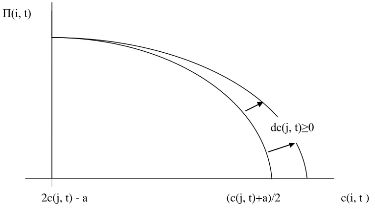
and similarly for firm j. dП(i, t)/dc(j, t) is positive (as long as П(i, t) > 0) and thus as rivals cost are lower so own profits are lower. Figure 1 illustrates the relationship of profits of firm i to own costs and the impact of an increase in rivals costs. In this Figure we see that, in the range where c(i,t) ≥ 2c(j,t) – a (i.e. where q(j,t) ≥ 0) and (c(j,t) + a)/2 ≥
5 If there is only one player (say firm i) in the market then that player may price as a monopolist charging
c(i,t) (where П(i, t) ≥ 0) and there are thus two players on the market6
, as c(i,t) increases so П(i, t) declines at an increasing rate from a maximum where c(i,t) = (2c(j,t) – a) to zero where c(i,t) = (c(j,t) + a)/2. We also observe that, for a given c(i,t), an increase in c(j,t) will increase the profits of firm i (by an increasing amount as c(i,t) increases).
[Figure 1 about here]
3. Strategic models of diffusion
Throughout we assume that there is an original technology, used by both firms, and a new cost reducing process technology that becomes available upon the market prior to time 1. This new technology is such that, for a given level of output, it will yield lower unit costs of production than the original technology, it requires, however, an investment by the firm in new capital goods. We assume any such investment in time t reduces unit production cost in time t + 1 (but not t), and the investment in the technology is
irreversible. We assume that c(i, 1) and c(j, 1) are inherited but that each firm may reduce its unit production cost in period 2 by ordering (installing) new technology in period 1 and the more new technology that is installed the lower will be second period productions costs. However, we provide structure to the modelling by assuming that in time period 1, firm i has already previously adopted the new technology to some extent but firm j has not. We make no attempt in this paper to provide a rationale as to why the first user is first or how the first user differs from the other firm. As lower cost levels for a firm (ceteris paribus) will reflect more extensive use of the new technology by that firm, the cost levels that a firm achieves in period 2 may be taken as indicators of the extent of intra firm diffusion in that firm at that point in time7.
3.1. A simple strategic model
6
Note that if c(i,t) equals (2c(j,t) – a) firm j will have zero output and leave the market.
7 Following convention, inter firm diffusion in time 2 could be measured by the proportion of firms that
In this section we build a simple game theoretic model of firm behaviour that reflects competitive rivalry but no spill over effects. We introduce such effects later below. In time period 1 firm i has to decide the extent to which to further invest in the new technology in order to enable further production cost reductions in period 2. Firm j in time period 1 must decide whether to invest in the new technology at all, and, if so, to what extent, so as to enable production using that technology in period 2. For the
benchmark case considered here, it is assumed that both firms have complete information upon the technology and the market when placing their orders for new technology and each can observe the investment orders placed by the other firm in time 1.
In determining the extent of use in the second period, each firm will compare the expected profit gains arising in the period 2 Nash equilibrium (where each firm expects the rival to act in a way that is in its own best interest) from lower costs in period 2 against the costs of investment in period 1 in order to generate those lower costs.
Defining the gain in profits for firm n as ∆П(n) and E(n) as the expenditure by firm n on new technology in time 1 to reduce costs in time 2, each firm will choose c(n, 2) such that the difference between ∆П(n) and E(n) is maximised i.e. where the marginal gross profit gain from investment equals the marginal cost8 of the investment9 i.e. where
d∆П(n)/dc(n,2) = dE(n)/ dc(n,2) for n = i and j.
From (5) we may state that
∆П(i)= ((a – 2c(i, 2)+ c(j, 2))2- (a – 2c(i, 1)+ c(j, i))2)/9b (11)
which yields that
d∆П(i)/dc(i,2)= -4(a – 2c(i, 2)+ c(j, 2))/9b (12)
8 This condition differs from that usually considered in diffusion models where the costs of new technology
are often considered independent of the extent of use and profit gains are compared with a fixed cost.
9 These are profitability criteria. If the cost of the new capital goods were falling over time there could also
and similarly for firm j.
The outcome of the modelling is critically dependent upon the determinants of the cost of installing new technology. Such costs will cover the cost of purchase of new machines, training costs, installation costs, adaptation costs etc. In this initial model we assume that such costs, labelled E(n), are proportional to the difference in the firms own costs of producing period 2 output at period 1 and period 2 unit production costs (i.e. for firm n, (c(n, 1) - c(n, 2))q(i, 2), such that
E(n) = α(n)(c(n, 1) - c(n, 2))q(n, 2) for c(n, 1) > c(n, 2) (13) = 0 otherwise
where α(n) is a positive constant less than unity (to ensure that the costs of adoption are less than the total production cost reductions) and may differ across firms. The
assumption that α(n) is a positive constant simplifies the analysis considerably, although it should be noted that in the investment literature it is often argued that adjustment costs are increasing in the investment undertaken (see for example, Nickell 1978). In the period 2 Nash equilibrium q(n, 2) are given by (2) and (3) which after substitution in (13) yields that, in the area of interest,
E(i) = α(i)((c(i, 1) - c(i, 2)).(a - 2c(i, 2) + c(j, 2))/3b (14)
E(j) = α(j)((c(j, 1) - c(j, 2)).(a - 2c(j, 2) + c(i, 2))/3b (15)
From which it is clear that
dE(i)/dc(i, 2) = α(i)(-2c(i, 1) - a + 4c(i, 2) - c(j, 2))/3b (16)
Setting d∆П(n)/dc(n,2) = dE(n)/ dc(n,2) for n = i, j then yields the following reaction curves for firm i and j
c(i,2) = [((a + c(j,2))(3α(i) - 4) + c(i,1)6α(i)]/(12 α(i) - 8) (18)
c(j,2) = [((a + c(i,2))(3α(j) - 4) + c(j,1)6α(j)]/(12 α(j) - 8) (19)
The second order conditions on the profit maximisation require that (12 α(n) - 8) > 0 i.e. (2/3) ≤ α(n) for n = i and j. Given also that, by construction, α(n) < 1 for n = i and j, it is required that α(n) satisfies (2/3) ≤ α(n) ≤ 1 implying that (3α(n) - 4)/(12 α(n) - 8) < 0 and 6α(n)/(12 α(j) - 8) > 0.
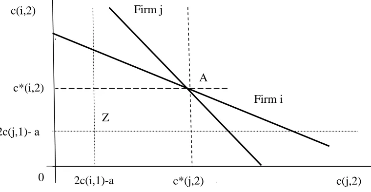
These reaction curves, indicating the choice of second period costs by firm i given the costs of firm j and vice versa, are both linear in the costs of the other firm. We note that, via (18), c(i,2) is negatively related to c(j,2) and, via (19), c(j,2) is negatively related to c(i,2) indicating that both reaction curves are downward sloping. This very much reflects the Reinganum (1981) argument that as one firm introduces new technology its output increases and this reduces the potential profit gains to other firms from introducing new technology. In Figure 2 we plot the reaction curves for firms i and j. The equilibrium (values indicated by a * superscript) occurs at the point of intersection, A.
[Figure 2 about here]
In this framework, and all the exercises that follow, we are only interested in those equilibria for which c(i,2) ≤ c(i,1) and c(j,2) ≤ c(j,1) i.e. where second period
It is clear that the extent of diffusion in the second period equilibrium depends upon the position and slopes of the two reaction curves and as such upon the parameters of the demand function (including therefore the elasticity of demand), first period costs and thus the extent of first period use by firm i, and α(i) and α(j) which incorporate the costs of purchasing and installing new machines. One might expect for example that if the costs of purchasing machines embodying new technology were to be lower in period 2 (ceteris paribus) then the equilibrium in period 2 would involve more extensive diffusion (lower costs for both firms).
It is clear that in a strategic framework such as this, the use of technology by one firm contemporaneously or concurrently is related to the use by rivals or other firms. This relationship is not however causal in any sense. The use by both firms at a given moment in time is determined as an outcome of the game and neither is causal to the other. Thus, although the sign of the impact of changes in exogenous variables and factors (e.g. a shift of the demand curve) upon c*(i, 2) and c*(j, 2) are the same, and thus one might expect c*(i, 2) and c*(j, 2) to be positively correlated, this will not be via a causal relationship.
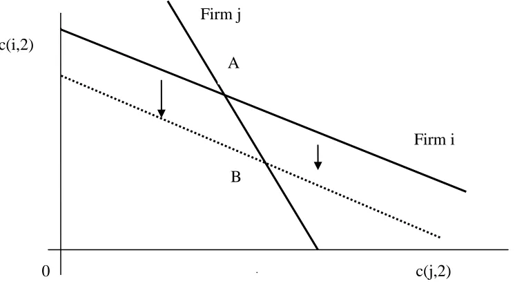
As the use by one firm of new technology is not contemporaneously causally related to the use by the other firm, in order to explore whether use by one firm impacts upon use by the other firm (positively or negatively) we need instead to explore whether, and or how, prior use, that is use in time t-1, which is determined independently of use in time t, will impact upon use in time t by both firms. The model is structured such that prior use is measured by c(i, 1), reflecting intra firm diffusion by firm i in the first period, and increases in prior use will be indicated by reductions in c(i,1).
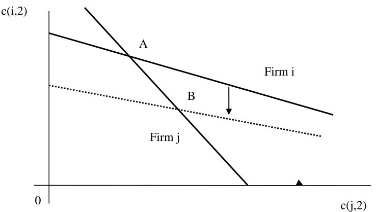
We may observe that a reduction in c(i, 1) will not affect the second period reaction curve for firm j but will shift down the reaction curve for firm i. As a result, the equilibrium will move as illustrated in Figure 3 from A to B. In the new equilibrium c*(i, 2) will be lower in the second period Nash equilibrium as a result of the greater usage by firm i in time 1 but c*(j, 2) will be greater10. Thus in terms of diffusion in this simple framework,
reflecting purely competitive rivalry between firms, the more extensive is one firm’s intra firm diffusion in the first period, the more intensively it will use that technology in the second period, but the less intensively will the rival use that technology in the second period. In essence this result derives from the fact that reduction in c(i, 1) leads to a lower level for c(i, 2) and higher output for firm i in time 2. This higher level of output reduces the profit gain available to firm j from reducing costs which leads to a higher level of c(j,2).
[Figure 3 about here]
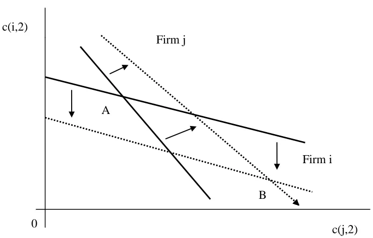
In order to facilitate analysis below it is useful at this stage to consider how changes in the costs of adoption of the new technology as represented by α(i) and α(j) impact upon the reactions curves (18) and (19) respectively. From (18) we may derive that an increase in α(i) increases the slope of the reaction curve for firm i, and also increases the intercept of that curve of the vertical axis (if a – 2c(i, 1) > 0) which is a condition for monopoly output in time 1 being positive). This shift of the reaction curve for firm i, along with the equivalent shift to the reaction curve for firm j when α(j) increases, is represented in Figure 4. Note that point Z (see Figure 2) is unaffected by these changes in α(i) and α(j).
[Figure 4 about here]
3.2. Early mover advantages
To initiate the consideration of whether spill over effects will affect how prior use will impact upon the current use of a new technology we proceed to consider a world in which there are first mover advantages or pre-emption effects (for an early discussion see Van der Werf and Mahon 1997) . The essence of pre-emption is that an incumbent (or innovating) firm may, by being the first mover, have a potential advantage relative to a second or later mover in any game11. The pre-emption effect in diffusion analysis is often
11 In an early study Lambkin (1988) shows that pioneers tend, on the average, to outperform later entrants
attributed to Fudenberg and Tirole (1985) and has been labelled the order effect in the inter firm literature. Most of such current relevant literature assumes however that when new technology is adopted it is adopted completely and there is no intra firm diffusion process. This essentially turns the pre-emption story into a one off timing game in which firms compete to be first in transforming 100% of their production processes to the new technology while the other firm(s) transform none (until some later date). It seems more reasonable to argue that the pre-emption effect is better suited to analysing intra firm diffusion, rather than first use. The game between firms would then relate to the relative extents of usage at different dates rather than the date of first usage. Lieberman and Montgomery (1988), for example allow that early mover effects may relate to extent of use. They also summarise the reasons for the existence of early mover advantages incorporating: proprietary learning effects, patents, pre-emption of input factors and locations, and development of buyer switching costs. Conversely, they also argue that early-mover disadvantages may result from free-rider problems, delayed resolution of uncertainty, shifts in technology or customer needs, and various types of organizational inertia. To proceed, we argue that the essence of early mover advantages is that an early mover may have the potential via its adoption decision to affect the intra firm diffusion decisions of later users. To model such first mover advantages effects we assume that as firm i uses the new technology more extensively in period 1 (and c(i, 1) is reduced) so the costs of acquisition by firm j increase (and this is known to firm i)12. Specifically we assume that α(j) in the costs of adoption of new technology by firm j is determined such that α(j) = F(c(i, 1)) with F > 0 and F’ < 0. Thus we have
E(i) = α(i)((c(i, 1) - c(i, 2)).(a - 2c(i, 2) + c(j, 2))/3b (14a)
E(j) = F(c(i, 1))((c(j, 1) - c(j, 2)).(a - 2c(j, 2) + c(i, 2))/3b (15a)
performance levels. Schnaars (1994) on the other hand argues that being an imitator is the best route. In a much more recent study Lanzolla et. al show that in the European mobile telephony market over the period 1998 to 2007 first and second movers consistently outperformed later entrants.
12 In a more complete model the choice of level of use by firm i in the first period would be at least partly
The reaction curve for firm i is unaffected (as 18a) but the reaction curve for firm j is now to be written as (19a).
c(i,2) = [((a + c(j,2))(3α(i) - 4) + c(i,1)6α(i)]/(12 α(i) - 8) (18a)
c(j,2) = [((a + c(i,2))(3 F(c(i,1)) - 4) + c(j,1)6F(c(i,1))]/(12 F(c(i,1)) - 8) (19a)
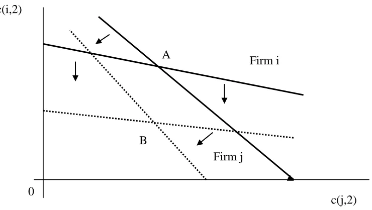
We maintain the previous assumption that (2/3) ≤ α(i) ≤ 1, but now, in order that for firm j both the costs of adoption are less than the production cost savings and the second order condition on the profit maximisation is met we must assume that (2/3) ≤ F(c(i,1)) ≤ 1, and thus 3F(c(i,1)) – 4 < 0 and 12 F(c(i,1)) – 8 > 0. The two reaction curves, shown in Figure 5 are then still downward sloping. The equilibrium again exists where the two reaction curves cross with an initial equilibrium at point A.
To explore the impact of prior diffusion on the equilibrium outcome we note that as c(i,1) is lower so the reaction curve for firm i moves down. However, the reduction in c(i,1), through pre-emption, increases F(c(i,1) because F’ < 0, and as it does so the reaction curve for firm j shifts as illustrated in Figure 4, with a new Nash equilibrium at point B in Figure 5. In essence we see that the pre-emption effect reinforces the direct effects of the reduction in c(i,1). In essence the stronger is the pre emption effect the lower will be c(i,2) and the higher will be c(j,2). In effect, just as in the benchmark model, with early mover advantages, increased prior usage by firm i does not encourage greater usage by firm j, in fact it discourages greater usage.
[Figure 5 about here]
3.3. Learning by doing
If there is learning by doing, own experience can reduce production costs via
(2011) have explored similar issues in the context of the diffusion of new energy
technologies. In the current context learning by doing may be modelled by allowing that the costs of production on the new technology in period 2 are dependent upon experience gained in period 1. We model this by arguing that the experience of the new technology in period 1 gained by firm i reduces its cost of attaining a lower production cost level in period 2 and thus allow that α(i) in the cost of adoption for firm i is determined such that α(i) = H(c(i, 1)) with H > 0 and H’ > 0, i.e. the greater is own past experience the cheaper it is to install the new technology. The cost of installation for firm j is not directly
affected i.e.
E(i) = H(c(i, 1)) ((c(i, 1) - c(i, 2)).(a - 2c(i, 2) + c(j, 2))/3b (14b)
E(j) = α(j) ((c(j, 1) - c(j, 2)).(a - 2c(j, 2) + c(i, 2))/3b (15b)
The reaction curves may then be written as
c(i,2) = [((a + c(j,2))(3 H(c(i, 1)) - 4) + c(i,1)6 H(c(i, 1))]/(12 H(c(i, 1)) - 8) (18b)
c(j,2) = [((a + c(i,2))(3α(j) - 4) + c(j,1)6α(j)]/(12 α(j) - 8) (19b)
and equilibrium occurs at the point of intersection of the two reaction curves (Figure 6, point A). In addition to assuming that (2/3) ≤ α(j) ≤ 1, we now assume that (2/3) ≤ H(c(i,1)) ≤ 1, in order that for firm i both the costs of adoption are less than the production cost savings and the second order condition on the profit maximisation is met. Thus 3H(c(i, 1)) - 4) < 0 and 12H(c(i, 1)) – 8 > 0. The reaction curves for c(i,2) and for c(j,2) are then again both downward sloping.
equilibrium will shift from A to B in Figure 6. Thus in the presence of a learning by doing spill-over it is still the case that that greater prior use by firm i in time 1 will generate higher use for that firm in time 2 and lower usage by firm j in time 2.
[Figure 6 about here]
3.4. Demonstration effects
Thus far we have not extensively discussed the knowledge set of the players in the games specified. However, there is a long tradition in the diffusion literature that argues that diffusion patterns to some degree at least reflect patterns of information or knowledge acquisition. There are two main parts to the information set. The first concerns
knowledge of existence of a new technology, the second concerns knowledge of the actual performance characteristics of that technology. The most common arguments are that: (i) non users observe users and by doing so learn of and/or about a technology; and (ii) firms learn from own experience on a technology as to the actual performance characteristics of that technology. Basically, use generates knowledge which in turn generates further use. This, it is argued, may generate a self-propagating diffusion process (see, for example, Mansfield 1968, Kapur 1995 and, Geroski 2000) exhibiting a bandwagon13.
While accepting that (i) as firms use a new technology they will learn about that
technology from their own experiences and (ii) that firms can learn of the existence of a new technology by observing that other firms are using that technology, it is difficult to accept that a firm will receive information upon the performance characteristics of a technology just by observing that another firm is using that technology. Current use will reflect past investment decisions rather than today’s information and as such will not necessarily be a good guide to current technology performance.
A better indicator of performance of a technology in time t would be orders placed for extensions of use by users in time t (i.e. planned intra firm diffusion). However because use by other firms will tend to lead to reductions in own profits, a firm whose
performance is being monitored by others will have an incentive to manipulate to its own advantage the signals that it sends. Intra firm diffusion therefore may well be subject to strategic behaviour because of the signals emanated. A firm investing in new technology therefore has to consider not only the basic rivalry effect which has been modelled, but also a demonstration effect, in that the firm’s own investment may encourage other firms to copy its behaviour and thus reduce its own return.
Assume that by using the new technology in period 1 at some (low) level firm i will learn the true performance characteristics of the technology before making its own investment decisions and thus those decisions will be fully informed. Firm j on the other hand, not having adopted the new technology by period 1, learns by observing firms i’s
orders/usage. But, for firm j, firm i’s investment plans are only an imperfect signal of the profitability to itself of investing in the new technology. The nature of the imperfection results from the fact that if firm i decides not to further invest in the new technology (or to invest only to a limited extent) firm j can take this as either (i) a signal that the new technology is inherently not (very) profitable, or (ii) that further investment in the new technology would not be profitable to firm i once the expected reaction and investment of firm j in the new technology takes place. Firm j cannot separate these two messages.
To reflect the situation assume that the investment costs of firm j include some search costs, and these search costs14 are lower the greater is the planned use of the new
technology by firm i. In particular we allow that α(j) = Ω(c(i, 2))where 0 < Ω(c(i, 2)) < 1 but increasing in c(i, 2)), the cost level chosen by firm i,and thus Ω’(c(i, 2)) > 0.This yields that
E(i) = α(i)((c(i, 1) - c(i, 2)).(a - 2c(i, 2) + c(j, 2))/3b (14c)
14 Such costs would also be lower if the firms are more alike in some sense. As a referee has pointed out, if
E(j) = Ω(c(i, 2))((c(j, 1) - c(j, 2)).(a - 2c(j, 2) + c(i, 2))/3b (15c)
The reaction curves may then be written as
c(i,2) = [((a + c(j,2))(3α(i) - 4) + c(i,1)6α(i)]/(12 α(i) - 8) (18c)
c(j,2) = [((a + c(i,2))(3 Ω(c(i, 2)) - 4) + c(j,1)6 Ω(c(i, 2))]/(12 Ω(c(i, 2)) - 8) (19c)
We assume as before that (2/3) ≤ α(i) ≤ 1 and thus (3α(i) - 4) < 0 and 12 α(i) – 8 > 0 and clearly the reaction curve for firm i is as before, being linear and downward sloping. The shape of the reaction curve for firm j will depend upon Ω(c(i, 2)). In general because
Ω’(c(i, 2)) > 0, the reaction curve for firm j will be non linear in c(i,2) and as c(i, 2) declines so the reaction curve for firm j will become steeper . We assume that (2/3) ≤ Ω(c(i, 2) ≤ 1, in order that, for firm j, the costs of adoption are always less than the
production cost savings and the second order condition on the profit maximisation is met. Thus 3Ω(c(i, 2)) - 4 < 0 and 12 Ω(c(i, 2)) - 8 > 0, and the reaction curve for firm j will, as
before, be downward sloping. The equilibrium occurs where the two reaction curves intersect. In Figure 7 we illustrate the case with an initial equilibrium at A.
[Figure 7 about here]
Reductions in c(i, 1) i.e. increases in prior use, shifts down the reaction curve for firm i. The reaction curve for firm j is not affected and the new equilibrium will exist at B. In the new equilibrium c(i,2) will be lower and c(j,2) will be higher but because the lower c(i,2) via demonstration effects reduces Ω(c(i, 2)), some of the increase in c(j,2) that would
have otherwise occurred is offset and c(j,2) increases by less than it would otherwise have done. Thus given the required restriction that (2/3) ≤ Ω(c(i, 2) ≤ 1, although
demonstration effects offset the effects of competitive rivalry, they do not outweigh these effects completely. This result is of special interest for, of all the spill over effects
(admittedly inter firm orientated) literature mainly relies for the existence of
bandwagons. Our results suggest that in a framework of competitive rivalry that may be too heroic a presumption.
We have also modelled a framework that allows for the firm to carry excess capacity and act as a predator in order to deter adoption by firm j. Not surprisingly this model also predicts that reduction in c(i, 1) increases own use and reduces rival use in period 2. As this is by now a standard result we do not report these results in detail. Instead we move to a situation where spill-overs may actually generate a bandwagon.
3.5. Network externalities
Whereas with learning by doing the beneficial impacts of prior use on production costs are private, if there are network effects then positive spill over effects benefits will be enjoyed by all users (for an empirical example see Goolsbee and Klenow 2002). In essence, with network effects, higher levels of use will benefit all users. To model a world with network effects we argue that such effects will not arise in period 1 but will arise in period 2 such that the lower is c(i, 1) the lower will be α(i) and α(j). We allow for this by assuming, in the simple way that α(i) = Hi(c(i, 1)) and α(j) = Hj(c(i, 1)) where Hi >
0, Hj > 0, Hi’ > 0 and Hj’ > 0 and thus
E(i) = Hi(c(i, 1)))((c(i, 1) - c(i, 2)).(a - 2c(i, 2) + c(j, 2))/3b (14d)
E(j) = Hj(c(i, 1)))((c(j, 1) - c(j, 2)).(a - 2c(j, 2) + c(i, 2))/3b (15d)
We may then write the reaction curves as (18d) and (19d).
c(i,2) = [((a + c(j,2))(3Hi(c(i, 1)) - 4) + c(i,1)6 Hi(c(i, 1))]/(12 Hi(c(i, 1)) - 8) (18d)
We assume that (2/3) ≤ Hi(c(i,1)) ≤ 1, and (2/3) ≤ Hj(c(j,1)) ≤ 1 in order that, for both
firms i and j, the costs of adoption are less than the production cost savings and the second order condition on the profit maximisation is met. Thus 3Hi(c(i, 1)) – 4 < 0,
3Hj(c(i, 1)) – 4 < 0, 12 Hi(c(i, 1)) – 8 > 0 and 12 Hj(c(i, 1)) – 8 > 0. Again both reaction
curves are then linear and downward sloping. Equilibrium will exist where the reaction curves intersect (initially point A in Figure 8).
[Figure 8 about here]
Greater prior use (a lower value for c(i, 1)) will shift the reaction curve for firm i downwards via the term in c(i, 1) which is reinforced via the terms in Hi(c(i, 1). The
reaction curve for firm j will not be affected directly by the change in c(i, 1) but will be shifted leftwards indirectly by the via the term in Hj(c(i, 1). In the new equilibrium c(i,2)
will be lower. If the indirect effect on firm j is strong enough it may also be that in the new equilibrium c(j,2) is lower than previously (as in Figure 8). Clearly the overall impact of greater prior use on c(i, 2) is negative but the impact on c(j,2) will depend upon the strength of the network effects. This is thus an example of how a spill over may produce a bandwagon in a model of competitive rivalry.
4. Discussion
It has not been our intention in the above to question whether, for example, there will be greater usage of new technology in a world where firms face network effects compared to a world in which firms have early mover advantages15. Instead the main purpose has been to explore, in a world in which firms strategically interact, how prior use of a new
technology by one firm will react upon the later use of new technology by itself and its rivals in the presence of different types of “spill overs” between firms. In the presence of such spill overs we ask whether prior use of a new technology by one firm will encourage or discourage further use by itself and other firms. Having argued that correlations in
15 Although this is a tempting question it is not at all clear what parameters should be standardised across
contemporaneous usage are not causal we consider the impact on the use in period 2 of changes in the production costs of the first adopter in period 1, c(i,1). Table 1 below provides a summary of the results derived above.
[Table 1 about here]
We find in all the models that changes in c(i,1) impact positively upon c(i,2) i.e. the greater is the use by the first user in period 1 the greater will be its use in the second period. This is not a surprising result given that investment is irreversible and prior investment reduces own later adoption costs. Of more interest however is how changes in c(i,1) impact upon c(j,2). Except when network externalities are very strong, the basic prediction is that greater intra firm usage by the innovator will reduce the intra firm usage of the follower in the second period. In essence the spill over effects either work in the same direction as the strategic forces or, if not, are overridden by the strategic forces.
The basic lesson is that the existence of spillovers in the diffusion process (even if positive in character) is not of itself sufficient to generate a bandwagon. The real impact of spillover effects can only be fully appreciated if they are considered within a model of competitive interaction between firms.
5. Conclusions
In the context of a simple two period, two firm model of strategic competition, we have explored how past use of new technology may impact upon current use via rivalrous behaviour and spill over effects and whether one may predict a bandwagon in the
diffusion process. Using the costs of the innovator in a first period, c(i,1), as a measure of prior intra firm diffusion, it has been shown that (except in the presence of strong
reinforced) by other spill over forces. Thus although there may be positive spill overs in the diffusion process, these are not necessarily sufficient to generate bandwagons overall because they are played out in a world of competitive interaction between firms.
Of course the modelling predictions that we have generated rely upon two basic
assumptions: that there are only two firms and that there are only two periods. Formally relaxing these assumptions would considerably complicate the analysis. In fact it might not even be possible to agree how some of the game theoretic approaches should be modelled if there are repeated games over time. Issues that might be more relevant in multi period multi player environments might be:
(i) At what stage do early mover advantages diminish or do they exist across the whole of the order of adoption?
(ii) How extensive are learning by doing, network and other spill over effects? (iii) To what extent as time proceeds will the number of users come to be a more
informative indicator of payoffs than the extent of use of each user? (iv) For how long can early users provide misleading signals to other potential
users as the number of users increases?
In addition, the models we have built are linear in construction. This was done for simplicity but there is no reason to believe that for example, demand curves are often linear (as opposed, say to constant elasticity). There may even be good reason to consider that some aspects of the models would be better modelled as non linear, for example, the costs of adoption may well vary non linearly with the extent of investments being undertaken,
The gap between the model and the real world also makes it problematic to consider whether there is any empirical support for the arguments presented in this paper. This is further complicated by the fact that there is only limited empirical literature on intra firm diffusion and also limited data. A rare source of intra firm data has been analysed in Battisti, Canepa and Stoneman (2009) which explored the third UK Community Innovation Survey (CIS3) data set relating to the use of e-business in the UK. They find for example that the probability that a firm in the sample chosen at random is a user of a new technology relates positively to both more use and more extensive use in the industry. In some ways this is not surprising, a positive relation with the number of users in the industry is very much to be expected (and almost a mathematical certainty), although it is not as obvious that there will be a positive relation with the average intensity of use (by users) in the industry. They also find that the probability of a firm chosen at random in an industry being an enhanced user is positively related to the average level of use (by users) in the industry, however this again is almost a mathematical certainty. Given in addition that the data is for a single cross section and thus does not offer information on lagged intra firm diffusion, it would seem overall that such empirical findings may have only limited relevance to the modelling undertaken here.
Such a policy would, ceteris paribus, tend to lead to lower levels for c(j,2) i.e. extend use by firm j. This would however be partly at the cost of discouraging further use by firm i, unless there are strong network effects. Such knock on effects should thus be considered as one of the possible effects of such policy intervention.
References
Arrow, K. J. 1962. The Economic Implications of Learning by Doing. The Review of Economic Studies, 29, no. 3:155- 173
Astebro, T. 2004. Sunk Costs and the Depth and Probability of Technology Adoption. Journal of Industrial Economics 52, no. 3: 381 – 99.
Battisti, G., Canepa, A. and Stoneman, P. 2009. E-Business usage across and within firms. Research Policy, 38, no.1: 133 – 143.
Battisti, G. and Stoneman, P. 2003. Inter Firm and Intra Firm Effects in the Diffusion of New Process Technologies. Research Policy 32, no.8: 1641-1655.
Battisti, G. and Stoneman, P. 2005. The Intra-Firm Diffusion of New Process Technologies. International Journal of Industrial Organisation, 23, no.1-2: 1-22.
Bollinger, B., and Gillingham, K. 2011. Peer Effects and Learning by Doing in the Diffusion of Solar Photovoltaic Panels. Working Paper, Yale University.
Fudenberg, D. and Tirole, J. 1985. Pre-emption and Rent Equalisation in the adoption of New Technology. Review of Economic Studies, 52, no .3: 383 – 401
Goolsbee, A. and Klenow P. J. 2002. Evidence On Learning And Network Externalities In The Diffusion Of Home Computers. Journal of Law and Economics, 45, no. 2: 317-343.
Ireland, N. and Stoneman, P. 1986. Technological Diffusion, Expectations and Welfare. Oxford Economic Papers, 38, no.2: 283 – 304.
Jackson, O. and Yariv, L. 2007. Diffusion of Behavior and Equilibrium Properties in Network Games. The American Economic Review (Papers and Proceedings), Volume 97. 2: 92-98.
Jovanovic, B. and Lach, S. 1989. Entry, Exit, and Diffusion with Learning by Doing, The American Economic Review, 79, no. 4: 690-699
Kapur, S. 1995. Technological Diffusion with Social Learning. Journal of Industrial Economics, 43, no.2: 173 – 95.
Katz, M. and Rosen, H. 1998. Microeconomics. McGraw-Hill, Boston Mass
Lambkin, M. 1988. Order of Entry and Performance in New Markets. Strategic Management Journal, 9(S1): 127-140.
Lanzolla, G., Gomez, J. and Maicas, J. P. 2010. Order of Market Entry, Market and Technological Evolution and Firm Competitive Performance. Paper presented at the DRUID Conference, Imperial College, London, June 16 – 18.
Mansfield, E. 1968. Industrial Research and Technological Innovation. New York, Norton.
Metcalfe, J. S. 1995. The Economic Foundations of Technology Policy: Equilibrium and Evolutionary Perspectives. In Handbook of the Economics of Innovation and
Technological Change, ed. P. Stoneman , 409 – 512. Oxford: Basil Blackwell
Nickell, S. 1978. The Investment Decisions of Firms. Cambridge, Nisbet.
Quirmbach, H. 1986. The Diffusion of New Technology and the Market for an Innovation. The Rand Journal of Economics, 17: 33 – 47
Reinganum, J. 1981. Market Structure and the Diffusion of New Technology. The Bell Journal of Economics, 12 no. 2: 618 – 24
Schnaars, S. P. 1994. Managing Imitation Strategies: How Late Entrants Seize Marketing from Pioneers. New York, Free Press.
Stoneman, P. 2002. The Economics of Technological Diffusion. Oxford, Basil Blackwell.
Stoneman, P. 2010. Soft Innovation: Economics, Product Aesthetics and the Creative Industries. Oxford, Oxford University Press.
Swann P. G. M. 2010. The Economics of Innovation. Edward Elgar, Cheltenham.
Table 1: Impact of increased first period use by firm i on second period use by firms i and j
Use by firm i Use by firm j
Basic model increased decreased
Early mover advantages increased decreased
Learning by doing increased decreased
Demonstration effects increased decreased
Illustration Captions
Figure 1: Gross profits and changes in own and rival’s unit costs of production Figure 2: The benchmark case
Figure 3: Pure rivalry: the impact of increased prior usage
Figure 4: The impact of increased adoption costs on reaction curves Figure 5: Early mover advantages
Figure 1: Gross profits and changes in own and rival’s unit costs of production
П(i, t)
c(i, t )
2c(j, t) - a (c(j, t)+a)/2
Figure 2: The benchmark case
Firm j c(i,2)
Firm i c*(i,2)
c*(j,2) A
Z
c(j,2) 2c(i,1)-a
2c(j,1)- a
Figure 3: Pure rivalry: the impact of increased prior usage
Firm j c(i,2)
Firm i B
A
Figure 4: The impact of increased adoption costs on reaction curves
Firm j c(i,2)
Firm i
Figure 5: Early mover advantages
Firm j c(i,2)
c(j,2) Firm i A
Figure 6: Learning by doing
Firm j c(i,2)
c(j,2) Firm i
A
B
Figure 7: Demonstration effects
Firm j
Firm i
A
B c(i,2)
Figure 8: Network effects
Firm j c(i,2)
c(j,2) Firm i
A
B