Optimal contracts for experimentation

warwick.ac.uk/lib-publications

Original citation:

Halac, Marina, Kartik, Navin and Liu, Qingmin. (2016) Optimal contracts for experimentation. Review of Economic Studies, 83 (3). pp. 1040-1091.

Permanent WRAP URL:

http://wrap.warwick.ac.uk/81646

Copyright and reuse:

The Warwick Research Archive Portal (WRAP) makes this work by researchers of the University of Warwick available open access under the following conditions. Copyright © and all moral rights to the version of the paper presented here belong to the individual author(s) and/or other copyright owners. To the extent reasonable and practicable the material made available in WRAP has been checked for eligibility before being made available.

Copies of full items can be used for personal research or study, educational, or not-for profit purposes without prior permission or charge. Provided that the authors, title and full bibliographic details are credited, a hyperlink and/or URL is given for the original metadata page and the content is not changed in any way.

Publisher’s statement:

This is a pre-copyedited, author-produced PDF of an article accepted for publication in Review of Economic Studies following peer review. The version of record is available online at: http://dx.doi.org/10.1093/restud/rdw013

A note on versions:

The version presented here may differ from the published version or, version of record, if you wish to cite this item you are advised to consult the publisher’s version. Please see the ‘permanent WRAP URL’ above for details on accessing the published version and note that access may require a subscription.

Optimal Contracts for Experimentation

∗

Marina Halac

†

Navin Kartik

‡

Qingmin Liu

§

January 13, 2016

Abstract

This paper studies a model of long-term contracting for experimentation. We consider a principal-agent relationship with adverse selection on the agent’s ability, dynamic moral haz-ard, and private learning about project quality. We find that each of these elements plays an essential role in structuring dynamic incentives, and it is only their interaction that generally precludes efficiency. Our model permits an explicit characterization of optimal contracts.

∗_{We thank Andrea Attar, Patrick Bolton, Pierre-Andr´e Chiappori, Bob Gibbons, Alex Frankel, Zhiguo He,} Supreet Kaur, Alessandro Lizzeri, Suresh Naidu, Derek Neal, Alessandro Pavan, Andrea Prat, Canice Prender-gast, Jonah Rockoff, Andy Skrzypacz, Lars Stole, Pierre Yared, various seminar and conference audiences, and anonymous referees and the Co-editor for helpful comments. We also thank Johannes H ¨orner and Gustavo Manso for valuable discussions of the paper. S´ebastien Turban provided excellent research assistance. Kartik gratefully acknowledges the hospitality of and funding from the University of Chicago Booth School of Business during a portion of this research; he also thanks the Sloan Foundation for financial support through an Alfred P. Sloan Fel-lowship.

†_{Graduate School of Business, Columbia University and Department of Economics, University of Warwick.} Email:[email protected].

Contents

1 Introduction 1

2 The Model 5

3 Benchmarks 8

3.1 The first best . . . 8

3.2 No adverse selection or no moral hazard . . . 9

4 Second-Best (In)Efficiency 11 5 Optimal Contracts whentH > tL 13 5.1 The solution . . . 13

5.2 Sketch of the proof . . . 17

5.3 Implications and applications . . . 20

6 Optimal Contracts whentH ≤tL 23 7 Discussion 28 7.1 Private observability and disclosure . . . 28

7.2 Limited liability . . . 28

7.3 The role of learning . . . 29

7.4 Adverse selection on other dimensions . . . 30

A Proof of Theorem 2 31

B Proof of Theorem 3 39

C Proof of Theorem 5 51

Bibliography 63

1. Introduction

Agents need to be incentivized to work on, or experiment with, projects of uncertain feasibility. Par-ticularly with uncertain projects, agents are likely to have some private information about their project-specific skills.1 Incentive design must deal with not only dynamic moral hazard, but also adverse selection (pre-contractual hidden information) and the inherent process of learning. To date, there is virtually no theoretical work on contracting in such settings. How well can a principal incentivize an agent? How do the environment’s features affect the shape of optimal incentive contracts? What distortions, if any, arise? An understanding is relevant not only for motivating research and development, but also for diverse applications like contract farming, technology adoption, and book publishing, as discussed subsequently.

This paper provides an analysis using a simple model of experimentation. We show that the inter-action of learning, adverse selection, and moral hazard introduces new conceptual and analytical issues, with each element playing a role in structuring dynamic incentives. Their interaction affects social effi-ciency: the principal typically maximizes profits by inducing an agent of low ability to end experimen-tation inefficiently early, even though there would be no distortion without either adverse selection or moral hazard. Furthermore, despite the intricacy of the problem, intuitive contracts are optimal. The principal can implement the second best by selling the project to the agent and committing to buy back output at time-dated future prices; these prices must increase over time in a manner calibrated to deal with moral hazard and learning.

Our model builds on the now-canonical two-armed “exponential bandit” version of experimentation (Keller, Rady, and Cripps, 2005).2 The project at hand may either be good or bad. In each period, the agent privately chooses whether to exert effort (work) or not (shirk). If the agent works in a period and the project is good, the project is successful in that period with some probability; if either the agent shirks or the project is bad, success cannot obtain in that period. In the terminology of the experimentation literature, working on the project in any period corresponds to “pulling the risky arm”, while shirking is “pulling the safe arm”; the opportunity cost of pulling the risky arm is the effort cost that the agent incurs. Project success yields a fixed social surplus, accrued by the principal, and obviates the need for any further effort. We introduce adverse selection by assuming that the probability of success in a period (conditional on the agent working and the project being good) depends on the agent’s ability—either high or low—which is the agent’s ex-ante private information or type. Our baseline model assumes no other contracting frictions, in particular we set aside limited liability and endow the principal with full ex-ante commitment power: she maximizes profits by designing a menu of contracts to screen the agent’s ability.3

1_{Other forms of private information, such as beliefs about the project feasibility or personal effort costs, are also}

relevant; seeSubsection 7.4.

2_{As surveyed byBergemann and V¨alim¨aki(2008), learning is often modeled in economics as an experimentation}

or bandit problem sinceRothschild(1974).

3_{Subsection 7.2studies the implications of limited liability. The importance of limited liability varies across}

Since beliefs about the project’s quality decline so long as effort has been exerted but success not ob-tained, the first-best or socially efficient solution is characterized by a stopping rule: the agent keeps work-ing (so long as he has not succeeded) up until some point at which the project is permanently abandoned. An important feature for our analysis is that the efficient stopping time is a non-monotonic function of the agent’s ability. The intuition stems from two countervailing forces: on the one hand, for any given belief about the project’s quality, a higher-ability agent provides a higher marginal benefit of effort because he succeeds with a higher probability; on the other hand, a higher-ability agent also learns more from the lack of success over time, so at any point he is more pessimistic about the project than the low-ability agent. Hence, depending on parameter values, the first-best stopping time for a high-ability agent may be larger or smaller than that of a low-ability agent (cf.Bobtcheff and Levy,2015).

Turning to the second best, the key distinguishing feature of our setting from a canonical (static) ad-verse selection problem is the dynamic moral hazard and its interaction with the agent’s private learning. Recall that in a standard buyer-seller adverse selection problem, there is no issue about what quantity the agent of one type would consume if he were to deviate and take the other type’s contract: it is simply the quantity specified by the chosen contract. By contrast, in our setting, it is nota prioriclear what “con-sumption bundle”, i.e. effort profile, each agent type will choose after such an off-the-equilibrium path deviation. Dealing with this problem would not pose any conceptual difficulty if there were a systematic relationship between the two types’ effort profiles, for instance if there were a “single-crossing condition” ensuring that the high type always wants to experiment at least as long as the low type. However, given the nature of learning, there is no such systematic relationship in an arbitrary contract. As effort off the equilibrium path is crucial when optimizing over the menu of contracts—because it affects how much “information rent” the agent gets—and the contracts in turn influence the agent’s off-path behavior, we are faced with a non-trivial fixed point problem.

Theorem 2establishes that the principal optimally screens the agent types by offering two distinct contracts, each inducing the agent to work for some amount of time (so long as success has not been ob-tained) after which the project is abandoned. Compared to the social optimum, an inefficiency typically obtains: while the high-ability type’s stopping time is efficient, the low-ability type experiments too little. This result is reminiscent of the familiar “no distortion at the top but distortion below” in static adverse selection models, but the distortion arises here only from the conjunction of adverse selection and moral hazard; we show that absent either one, the principal would implement the first best (Theorem 1). More-over, because of the aforementioned lack of a single-crossing property, it is not immediate in our setting that the principal shouldn’t have the low type over-experiment to reduce the high type’s information rent, particularly when the first best entails the high type stopping earlier than the low type.

analog of the single-crossing condition mentioned above in an arbitrary contract, such a condition must hold in anoptimalcontract for the low type. This allows us to simplify the problem and fully characterize the principal’s solution (Theorem 3 andTheorem 4). The case in which the first-best stopping time for the high-ability agent is lower than that of the low-ability agent proves to be more challenging: now, as suggested by the first best, an optimal contract for the low type is often such that the high type would experiment less than the low type should he take this contract. We are able to fully characterize the solution in this case under no discounting (Theorem 5andTheorem 6).

The second-best contracts we characterize take simple and intuitive forms, partly owing to the simple underlying primitives. In any contract that stipulates experimentation forT periods it suffices to consider at most T + 1 transfers. The reason is that the parties share a common discount factor and there are

T + 1 possible project outcomes: a success can occur in each of the T periods or never. One class of contracts are bonus contracts: the agent pays the principal an up-front fee and is then rewarded with a bonus that depends on when the project succeeds (if ever). We characterize the unique sequence of time-dependent bonuses that must be used in an optimal bonus contract for the low-ability type.4 This sequence is increasing over time up until the termination date. The shape, and its exact calibration, arises from a combination of the agent becoming more pessimistic over time (absent earlier success) and the principal’s desire to avoid any slack in the provision of incentives, while crucially taking into account that the agent can substitute his effort across time.

The optimal bonus contract can be viewed as a simple “sale-with-buyback contract”: the principal sells the project to the agent at the outset for some price, but commits to buy back the project’s output (that obtains with a success) at time-dated future prices. It is noteworthy that contract farming arrangements, widely used in developing countries between agricultural companies and farm producers (Barrett et al.,

2012), are often sale-with-buyback contracts: the company sells seeds or other technology (e.g., fertilizers or pesticides) to the farmer and agrees to buy back the crop at pre-determined prices, conditional on this output meeting certain quality standards and delivery requirements (Minot,2007). The contract farming setting involves a profit-maximizing firm (principal) and a farmer (agent). Miyata, Minot, and Hu(2009) describe the main elements of these environments, focusing on the case of China. It is initially unknown whether the new seeds or technology will produce the desired outcomes in a particular farm, which maps into our project uncertainty.5 _{Besides the evident moral hazard problem, there is also adverse} selection: farmers differ in unobservable characteristics, such as industriousness, intelligence, and skills.6 Our analysis not only shows that sale-with-buyback contracts are optimal in the presence of uncertainty, moral hazard, and unobservable heterogeneity, but elucidates why. Moreover, as discussed further in

4_{For the high type, there are multiple optimal contracts even within a given class such as bonus contracts.}

The reason for the asymmetry is that the low type’s contract is pinned down by information rent minimization considerations, unlike the high type’s contract. Of course, the high type’s contract cannot be arbitrary either.

5_{Besley and Case(1993) study how farmers learn about a new technology over time given the realization of}

yields from past planting decisions, and how they in turn make dynamic choices.

Subsection 5.3, our paper offers implications for the design of such contracts and for field experiments on technology adoption more broadly. In particular, field experiments might test our predictions regarding the rich structure of optimal bonus contracts and how the calibration depends on underlying parameters.7

Another class of optimal contracts that we characterize arepenalty contracts: the agent receives an up-front payment and is then required to pay the principal some time-dependent penalty in each period in which a success does not obtain, up until either the project succeeds or the contract terminates.8 Analo-gous to the optimal bonus contract, we identify the unique sequence of penalties that must be used in an optimal penalty contract for the low-ability type: the penalty increases over time with a jump at the ter-mination date. These types of contracts correspond to those used, for example, in arrangements between publishers and authors: authors typically receive advances and are then required to pay the publisher back if they do not succeed in completing the book by a given deadline (Owen,2013). This application fits into our framework when neither publisher nor author may initially be sure whether a commercially-viable book can be written in the relevant timeframe (uncertain project feasibility); the author will have superior information about his suitability or comparative advantage in writing the book (adverse selec-tion about ability); and how much time he actually devotes to the task is unobservable (moral hazard).9

Our results have implications for the extent of experimentation and innovation across different eco-nomic environments. An immediate prediction concerns the effects of asymmetric information: we find that environments with more asymmetric information (either moral hazard or adverse selection) should feature less experimentation, lower success rates, and more dispersion of success rates. We also find that the relationship between success rates and the underlying environment can be subtle. Absent any dis-tortions, “better environments” lead to more innovation. Specifically, an increase in the proportion of high-ability agents or an increase in the ability of both types of the agent yields a higher probability of success in the first best. In the presence of moral hazard and adverse selection, however, the opposite can be true: these changes can induce the principal to distort the low-ability type’s experimentation by more, to the extent that the average success probability goes down in the second best. Consequently, observing higher innovation rates in contractual settings like those we study is neither necessary nor sufficient to deduce a better underlying environment. As discussed inSubsection 5.3, these results may contribute an agency-theoretic component to the puzzle of low technology adoption rates in developing countries.

Related literature. Broadly, this paper fits into literatures on long-term contracting with either dynamic

7_{We should highlight that our paper is not aimed at studying all the institutional details of contract farming or}

technology adoption. For example, we do not address multi-agent experimentation and social learning, which has been emphasized by the empirical literature (e.g.,Conley and Udry,2010).

8_{There is a flavor here of “clawbacks” that are sometimes used in practice when an agent is found to be negligent.}

In our setting, it is the lack of project success that is treated like evidence of negligence (i.e. shirking); note, however, that in equilibrium the principal knows that the agent is not actually negligent.

9_{Not infrequently, authors fail to deliver in a timely fashion (Suddath,2012). That private information can be}

moral hazard and/or adverse selection. Few papers combine both elements, but two recent excep-tions areSannikov(2007) andGershkov and Perry(2012).10 _{These papers are not concerned with} learn-ing/experimentation and their settings and focus differ from ours in many ways.11 More narrowly, start-ing withBergemann and Hege(1998,2005), there is a fast-growing literature on contracting for experimen-tation. Virtually all existing research in this area addresses quite different issues than we do, primarily because adverse selection is not accounted for.12 _{The only exception we are aware of is the concurrent} work ofGomes, Gottlieb, and Maestri(2015). They do not consider moral hazard; instead, they introduce two-dimensional adverse selection. Under some conditions they obtain an “irrelevance result” on the dimension of adverse selection that acts similar to our agent’s ability, a conclusion that is similar to our benchmark that the first best obtains in our model when there is no moral hazard.

Outside a pure experimentation framework, Gerardi and Maestri(2012) analyze how an agent can be incentivized to acquire and truthfully report information over time using payments that compare the agent’s reports with the ex-post observed state; by contrast, we assume the state is never observed when experimentation is terminated without a success. Finally, our model can also be interpreted as a problem of delegated sequential search, as inLewis and Ottaviani(2008) andLewis(2011). The main difference is that, in our context, these papers assume that the project’s quality is known and hence there is no learning about the likelihood of success (cf.Subsection 7.3); moreover, they do not have adverse selection.

2. The Model

Environment.A principal needs to hire an agent to work on a project. The project’s quality—synonymous with the state—may either be good or bad, a binary variable. Both parties are initially uncertain about the project’s quality; the common prior on the project being good isβ0 ∈ (0,1). The agent is privately

informed about whether his ability is low or high, θ _{∈ {}L, H_}, where θ = H represents “high”. The principal’s prior on the agent’s ability being high isµ0 ∈(0,1). In each period,t ∈ {1,2, . . .}, the agent

can either exert effort (work) or not (shirk); this choice is never observed by the principal. Exerting effort

10_{Some earlier papers with adverse selection and dynamic moral hazard, such asLaffont and Tirole(1988), focus}

on the effects of short-term contracting. There is also a literature on dynamic contracting with adverse selection and evolving types but without moral hazard or with only one-shot moral hazard, such asBaron and Besanko(1984) or, more recently,Battaglini(2005),Boleslavsky and Said(2013), andEs˝o and Szentes(2015).Pavan, Segal, and Toikka (2014) provide a rather general treatment of dynamic mechanism design without moral hazard.

11_{Demarzo and Sannikov(2011),He et al.(2014), andPrat and Jovanovic(2014) study private learning in}

moral-hazard models followingHolmstr ¨om and Milgrom(1987), but do not have adverse selection. Sannikov(2013) also proposes a Brownian-motion model and a first-order approach to deal with moral hazard when actions have long-run effects, which raises issues related to private learning. Chassang(2013) considers a general environment and develops an approach to find detail-free contracts that are not optimal but instead guarantee some efficiency bounds so long as there is a long horizon and players are patient.

12_{SeeBonatti and H ¨orner(2011,2015),Manso(2011),Klein(2012),Ederer(2013),H ¨orner and Samuelson(2013),}

in any period costs the agentc >0. If effort is exerted and the project is good, the project is successful in that period with probabilityλθ; if either the agent shirks or the project is bad, success cannot obtain in that period. Success is observable and once a project is successful, no further effort is needed.13 We assume

1> λH > λL>0. A success yields the principal a payoff normalized to1; the agent does not intrinsically care about project success. Both parties are risk neutral, have quasi-linear preferences, share a common discount factorδ ∈(0,1], and are expected-utility maximizers.

Contracts. We consider contracting at period zero with full commitment power from the principal. To deal with the agent’s hidden information at the time of contracting, the principal’s problem is, without loss of generality, to offer the agent amenu of dynamic contracts from which the agent chooses one. A dynamic contract specifies a sequence of transfers as a function of the publicly observable history, which is simply whether or not the project has been successful to date. To isolate the effects of adverse selection, we do not impose any limited liability constraints untilSubsection 7.2. We assume that once the agent has accepted a contract, he is free to work or shirk in any period up until some termination date that is specified by the contract.14 Throughout, we follow the convention that transfers are from the principal to the agent; negative values represent payments in the other direction.

Formally, acontractis given byC= (T, W0,b,l), whereT ∈N≡ {0,1, . . .}is thetermination dateof the contract,W0 ∈Ris an up-front transfer (or wage) at period zero,b= (b1, . . . , bT)specifies a transferbt∈R made at periodtconditional on the project being successful in periodt, and analogouslyl= (l1, . . . , lT)

specifies a transferlt∈Rmade at periodtconditional on the project not being successful in periodt(nor in any prior period).15,16_{We refer to anyb}

tas abonusand anyltas apenalty. Note thatbtis not constrained

to be positive nor mustltbe negative; however, these cases will be focal and hence our choice of

termi-nology. Without loss of generality, we assume that ifT > 0thenT = max_{t:eitherbt6= 0orlt6= 0}. The

agent’s actions are denoted bya= (a1, . . . , aT), whereat= 1if the agent works in periodtandat= 0if

the agent shirks.

Payoffs. The principal’s expected discounted payoff at time zero from a contractC = (T, W0,b,l), an

13_{Subsection 7.1establishes that our results apply without change if success is privately observed by the agent}

but can be verifiably disclosed.

14_{There is no loss of generality here. If the principal has the ability to block the agent from choosing whether to}

work in some period—“lock him out of the laboratory”, so to speak—this can just as well be achieved by instead stipulating that project success in that period would trigger a large payment to the principal.

15_{We thus restrict attention to deterministic contracts. Throughout, symbols in bold typeface denote vectors.W}

0

andT are redundant becauseW0can be effectively induced by suitable modifications tob1andl1, whileT can be

effectively induced by settingbt = lt = 0for allt > T. However, it is expositionally convenient to include these

components explicitly in defining a contract. Furthermore, there is no loss in assuming thatT _∈N; as we show, it is always optimal for the principal to stop experimentation at a finite time, so she cannot benefit from settingT =_∞.

16_{As the principal and agent share a common discount factor, what matters is only the mapping from outcomes}

agent of typeθ, and a sequence of the agent’s actionsais denotedΠθ₀(C,a), which can be computed as:

Πθ₀(C,a) :=₋W0−(1−β0) T

X

t=1

δtlt+β0 T

X

t=1

δt "

Y

s<t

1₋asλθ

#h

atλθ(1−bt)−

1₋atλθ

lt

i

. (1)

Formula (1) is understood as follows. W0 is the up-front transfer made from the principal to the agent.

With probability1₋β0 the state is bad, in which case the project never succeeds and hence the entire

sequence of penalties l is transferred. Conditional on the state being good (which occurs with proba-bility β0), the probability of project success depends on both the agent’s effort choices and his ability;

Q

s<t

1−asλθ

is the probability that a success does not obtain between period1andt−1conditional on

the good state. If the project were to succeed at timet, then the principal would earn a payoff of1in that period, and the transfers would be the sequence of penalties(l1, . . . , lt−1)followed by the bonusbt.

Through analogous reasoning, bearing in mind that the agent does not directly value project success but incurs the cost of effort, the agent’s expected discounted payoff at time zero given his typeθ, contract

C, and action profileais

U₀θ(C,a) :=W0+ (1−β0) T

X

t=1

δt(lt−atc) +β0 T

X

t=1

δt "

Y

s<t

1₋asλθ

#h at

λθbt−c

+1₋atλθ

lt

i . (2)

If a contract is not accepted, both parties’ payoffs are normalized to zero.

Bonus and penalty contracts. Our analysis will make use of two simple classes of contracts. A bonus

contractis one where aside from any initial transfer there is at most only one other transfer, which occurs

when the agent obtains a success. Formally, a bonus contract isC= (T, W0,b,l)such thatlt= 0for allt∈ {1, . . . , T_}. A bonus contract is aconstant-bonus contractif, in addition, there is some constantbsuch that

bt =bfor allt∈ {1, . . . , T}. When the context is clear, we denote a bonus contract as justC= (T, W0,b)

and a constant-bonus contract as C= (T, W0, b). By contrast, a penalty contractis one where the agent

receives no payments for success and instead is penalized for failure. Formally, a penalty contract is

C= (T, W0,b,l)such thatbt= 0for allt ∈ {1, . . . , T}. A penalty contract is aonetime-penalty contractif,

in addition,lt = 0for allt ∈ {1, . . . , T −1}. That is, while in a general penalty contract the agent may

be penalized for each period in which he fails to obtain a success, in a onetime-penalty contract the agent is penalized only if a success does not obtain by the termination dateT. We denote a penalty contract as justC= (T, W0,l)and a onetime-penalty contract asC= (T, W0, lT).

Although each of these two classes of contracts will be useful for different reasons, there is an iso-morphism between them; furthermore, either class is “large enough” in a suitable sense. More precisely, say that two contracts, C = (T, W0,b,l) andCb = (T,Wc0,bb,bl), are equivalent if for all θ ∈ {L, H} and

Proposition 1. For any contractC= (T, W0,b,l)there exist both an equivalent penalty contractCb = (T,Wc0,bl)

and an equivalent bonus contractCe = (T,Wf0,eb).

Proof. See theSupplementary Appendix. Q.E.D.

Proposition 1implies that it is without loss to focus either on bonus contracts or on penalty contracts. The proof is constructive: given an arbitrary contract, it explicitly derives equivalent penalty and bonus contracts. The intuition is that all that matters in any contract is the induced vector of discounted trans-fers for success occurring in each possible period (and never), and these transtrans-fers can be induced with bonuses or penalties.17 The proof also shows that whenδ = 1, onetime-penalty contracts are equivalent to constant-bonus contracts.

3. Benchmarks

3.1. The first best

Consider the first-best solution, i.e. when the agent’s type θis commonly known and his effort in each period is publicly observable and contractible. Since beliefs about the state being good decline so long as effort has been exerted but success not obtained, the first-best solution is characterized by a stopping rule such that an agent of abilityθkeeps exerting effort so long as success has not obtained up until some periodtθ, whereafter effort is no longer exerted.18Letβ_tθbe a generic belief on the state being good at the beginning of periodt(which will depend on the history of effort), and βθ_t be this belief when the agent has exerted effort in all periods1, . . . , t₋1. The first-best stopping timetθis given by

tθ = max

t≥0

n

t:βθ_tλθ _≥c o

, (3)

where, for eachθ,βθ₀ :=β0, and fort≥1, Bayes’ rule yields

βθ_t = β0 1−λ

θt−1

β0(1−λθ)t−1+ (1−β0)

. (4)

17_{For example, in a two-period contractC= (2, W}

0,b,l), the agent’s discounted transfer isW0+δb1if he succeeds

in period one,W0+δl1+δ2b2 if he succeeds in period two, andW0+δl1+δ2l2 if he does not succeed in either

period. The same transfers are induced by a penalty contractCb = (2,Wc0,bl)withcW0=W0+δb1,bl1=l1−b1+δb2,

andbl2=l2−b2, and by a bonus contractCe = (2,Wf0,eb)withWf0=W0+δl1+δ2l2,eb1=b1−l1−δl2, andeb2=b2−l2.

18_{More precisely, the first best can always be achieved using a stopping rule for each type; when and only when}

Note that (3) is only well-defined whenc≤β0λθ; ifc > β0λθ, it would be efficient to not experiment

at all, i.e. stop attθ = 0. To focus on the most interesting cases, we assume:

Assumption 1. Experimentation is efficient for both types: forθ_{∈ {}L, H_},β0λθ > c.

If parameter values are such that βθ_tθλθ = c,19 equations (3) and (4) can be combined to derive the

following closed-form solution for the first-best stopping time for typeθ:

tθ= 1 +

log_λθc_−c

1−β0

β0

log (1−λθ₎ . (5)

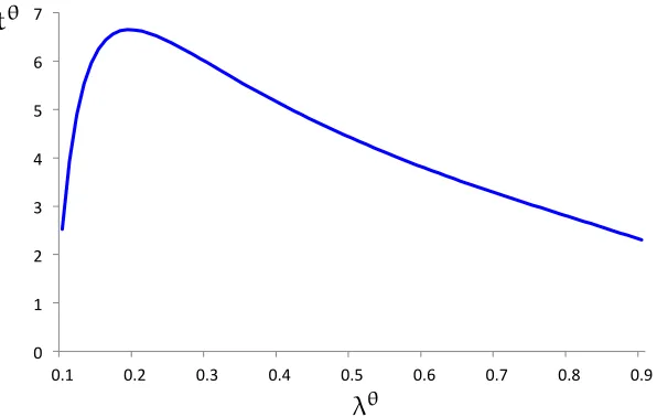
Equation (5) yields intuitive monotonicity of the first-best stopping time as a function of the prior that the project is good, β0, and the cost of effort, c.20 But it also implies a fundamental non-monotonicity

as a function of the agent’s ability, λθ, as shown inFigure 1. (For simplicity, the figure ignores integer constraints ontθ.) This stems from the interaction of two countervailing forces. On the one hand, for any given belief about the state, the expected marginal benefit of effort is higher when the agent’s ability is higher; on the other hand, the higher is the agent’s ability, the more informative is a lack of success in a period in which he works. Hence, at any timet > 1, a higher-ability agent is more pessimistic about the state (given that effort has been exerted in all prior periods), which has the effect of decreasing the expected marginal benefit of effort. Altogether, this makes the first-best stopping time non-monotonic in ability; bothtH > tL andtH < tLare robust possibilities that arise for different parameters. As we will see, this has substantial implications.

The first-best expected discounted surplus at time zero from typeθis

tθ

X

t=1

δt

β0

1₋λθt

−1

λθ₋c₋(1₋β0)c

.

3.2. No adverse selection or no moral hazard

Our model has two sources of asymmetric information: adverse selection and moral hazard. To see that their interaction is essential, it is useful to understand what would happen in the absence of either one.

Consider first the case without adverse selection, i.e. assume the agent’s ability is observable but there is moral hazard. The principal can then use a constant-bonus contract to effectively sell the project to the agent at a price that extracts all the (ex-ante) surplus. Specifically, suppose the principal offers the agent

19_{We do not assume this condition in our analysis, but it is convenient for the current discussion.}

20_{One may also notice that the discount factor,δ, does not enter (5). In other words, unlike the traditional focus}

0" 1" 2" 3" 4" 5" 6" 7"

0.1" 0.2" 0.3" 0.4" 0.5" 0.6" 0.7" 0.8" 0.9"

First Best

First best

characterized by optimal stopping time

t

✓

:

t

✓

=

max

t>0

⌦

t

:

✓t ✓

>

c

↵

,

where

✓_t

is belief on good state at beginning of

t

given work up to

t

Assumption 1

. Experimentation is efficient: for

✓

₂

{

L

,

H

}

,

0 ✓

> c

.

Note both

t

H

> t

L

and

t

H

< t

L

are robust possibilities

!

Productivity vs. learning e↵ects:

• For given belief on good state, marginal benefit of e↵ort higher for H

• But at any point in time, given no success, belief lower for H

Model – Environment (2)

In each period

t

2

{

1, 2, . . .

}

, agent covertly chooses to work or shirk

• Exerting e↵ort in any period costs the agentc >0

If agent works and state is good, project succeeds with probability

✓

• 1> H> L >0

If agent shirks or state is bad, success cannot obtain

Project success yields principal payo↵ normalized to 1

• No further e↵ort once success is obtained

Project success is publicly observable

[image:13.612.158.456.53.242.2]

• Results also hold if privately observed by agent but verifiable disclosure

Figure 1–The first-best stopping time.

of typeθa constant-bonus contractCθ = (tθ, W₀θ,1), whereW₀θis chosen so that conditional on the agent exerting effort in each period up to the first-best termination date (as long as success has not obtained), the agent’s participation constraint at time zero binds:

U₀θCθ,1=

tθ

X

t=1

δt

β0

1₋λθt−1λθ₋c₋(1₋β0)c

+W₀θ = 0,

where the notation 1denotes the action profile of working in every period of the contract. Plainly, this contract makes the agent fully internalize the social value of success and hence achieves the first-best level of experimentation, while the principal keeps all the surplus.

Consider next the case with adverse selection but no moral hazard: the agent’s effort in any period still costs himc > 0but is observable and contractible. The principal can then implement the first best and extract all the surplus by using simple contracts that pay the agent for effort rather than outcomes. Specifically, the principal can offer the agent a choice between two contracts that involve no bonuses or penalties, with each paying the agentcfor every period that he works. The termination date istLin the contract intended for the low type andtH in the contract intended for the high type. Plainly, the agent’s payoff is zero regardless of his type and which contract and effort profile he chooses. Hence, the agent is willing to choose the contract intended for his type and work until either a success is obtained or the termination date is reached.21

To summarize:

21_{The same idea underliesGomes et al.’s (2015) Lemma 2. While this mechanism makes the agent indifferent}

Theorem 1. If there is either no moral hazard or no adverse selection, the principal optimally implements the first best and extracts all the surplus.

A proof is omitted in light of the simple arguments preceding the theorem.Theorem 1also holds when there are many types; that both kinds of information asymmetries are essential to generate distortions is general in our experimentation environment.22

4. Second-Best (In)Efficiency

We now turn to the setting with both moral hazard and adverse selection. In this section, we formalize the principal’s problem and deduce the nature of second-best inefficiency. We provide explicit character-izations of optimal contracts inSection 5andSection 6.

Without loss, we assume that the principal specifies a desired effort profile along with a contract. An optimal menu of contracts maximizes the principal’s ex-ante expected payoff subject to incentive compatibility constraints for effort (ICθa below), participation constraints (IRθ below), and self-selection

constraints for the agent’s choice of contract (ICθθ0 below). Denote

αθ(C) := arg max a

U₀θ(C,a)

as the set of optimal action plans for the agent of typeθunder contractC. With a slight abuse of notation, we will writeUθ

0(C,αθ(C))for the type-θagent’s utility at time zero from any contractC. The principal’s

program is:

max

(CH_,CL_,aH_,aL₎µ0Π

H

0 CH,aH

+ (1₋µ0) ΠL0 CL,aL

subject to, for allθ, θ0 _{∈ {}L, H_},

aθ ∈αθ(Cθ), (ICθ

a)

U₀θ(Cθ,aθ)_≥0, (IRθ)

U₀θ(Cθ,aθ)_≥U₀θ(Cθ0,αθ(Cθ0)). (ICθθ0)

Adverse selection is reflected in the self-selection constraints (ICθθ0_{), as is familiar. Moral hazard is}

reflected directly in the constraints (ICθ

a) and also indirectly in the constraints (ICθθ

0

) via the termαθ(Cθ0). To get a sense of how these matter, consider the agent’s incentive to work in some periodt. This is shaped not only by the transfers that are directly tied to success/failure in period t(bt andlt) but also by the

22_{We note that learning is also important in generating distortions: in the absence of learning (i.e. if the project}

were known to be good,β0 = 1), the principal may again implement the first best. For expositional purposes, we

transfers tied to subsequent outcomes, through their effect on continuation values. In particular, ceteris

paribus, raising the continuation value (say, by increasing eitherbt+1 orlt+1) makes reaching periodt+ 1

more attractive and hence reduces the incentive to work in periodt: this is a dynamic agency effect.23 Note moreover that the continuation value at any point in a contract depends on the agent’s type and his effort profile; hence it is not sufficient to consider a single continuation value at each period. Furthermore, besides having an effect on continuation values, the agent’s type also affects current incentives for effort because the expected marginal benefit of effort in any period differs for the two types. Altogether, the optimal plan of action will generally be different for the two types of the agent, i.e. for an arbitrary contract

C, we may haveαH(C)_∩αL(C) =_∅.24

Our result on second-best (in)efficiency is as follows:

Theorem 2. In any optimal menu of contracts, each type θ _{∈ {}L, H_} is induced to work for some number of

periods,tθ. Relative to the first-best stopping times,tH _andtL_{, the second best hast}H _=tH _andtL_≤tL_.

Proof. SeeAppendix A. Q.E.D.

Theorem 2says that relative to the first best, there is no distortion in the amount of experimentation by the high-ability agent whereas the low-ability agent may be induced to under-experiment. It is interesting that this is a familiar “no distortion (only) at the top” result from static models of adverse selection, even though the inefficiency arises here from the conjunction of adverse selection and dynamic moral hazard (cf. Theorem 1). Moral hazard generates an “information rent” for the high type but not for the low type. As will be elaborated subsequently, reducing the low type’s amount of experimentation allows the principal to reduce the high type’s information rent. The optimaltLtrades off this information rent with the low type’s efficiency. For typical parameters, it will be the case thattL _{∈ {}1, . . . , tL_{−1}, so that the}

low type engages in some experimentation but not as much as socially efficient; however, it is possible that the low type is induced to not experiment at all (tL= 0) or to experiment for the first-best amount of time (tL=tL). The former possibility arises for reasons akin to exclusion in the standard model (e.g. the prior,µ0, on the high type is sufficiently high); the latter possibility is because time is discrete. Indeed, if

the length of each time interval shrinks and one takes a suitable continuous-time limit, then there will be some distortion, i.e.tL< tL.

The proof ofTheorem 2does not rely on characterizing second-best contracts.25 We establishtH =tH

23_{Mason and V¨alim¨aki(2011),Bhaskar(2012,2014),H ¨orner and Samuelson(2013), andKwon(2013) also}

high-light dynamic agency effects, but in settings without adverse selection.

24_{Related issues arise in static models that allow for both adverse selection and moral hazard; see for example}

the discussion inLaffont and Martimort(2001, Chapter 7).

25_{Note that whenδ <1, efficiency requires each type to use a “stopping strategy” (i.e., work for a consecutive}

by proving that the low type’s self-selection constraint can always be satisfied without creating any distor-tions. The idea is that the principal can exploit the two types’ differing probabilities of success by making the high type’s contract “risky enough” to deter the low type from taking it, while still satisfying all other constraints.26 We establishtL_≤tL by showing that any contract for the low type inducingtL > tLcan be modified by “removing” the last period of experimentation in this contract and concurrently reducing the information rent for the high type. Due to the lack of structure governing the high type’s behav-ior upon deviating to the low type’s contract, we prove the information-rent reduction no matter what action plan the high type would choose upon taking the low type’s contract. It follows that inducing over-experimentation by the low type cannot be optimal: not only would that reduce social surplus but it would also increase the high type’s information rent.

WhileTheorem 2has implications for the extent of experimentation and innovation in different eco-nomic environments, we postpone such discussion toSubsection 5.3, after describing optimal contracts and their comparative statics.

5. Optimal Contracts when

t

H

> t

L

We characterize optimal contracts by first studying the case in which the first-best stopping times are orderedtH > tL, i.e. when the speed-of-learning effect that pushes the first-best stopping time down for a higher-ability agent does not dominate the productivity effect that pushes in the other direction. Any of the following conditions on the primitives is sufficient fortH > tL, given a set of other parameters: (i)β0

is small enough, (ii)λLandλH are small enough, or (iii)cis large enough. We maintain the assumption thattH > tLimplicitly throughout this section.

5.1. The solution

A class of solutions to the principal’s program described inSection 4whentH > tLis as follows:

26_{Specifically, given an optimal contract for the high type, the principal can increase the magnitude of the}

penal-ties while adjusting the time-zero transfer so that the high type’s expected payoff and effort profile do not change. Making the penalties severe enough (i.e., negative enough) then ensures that the low type’s payoff from taking the high type’s contract is negative and hence (ICLH_{) is satisfied at no cost. Crucially, an analogous construction would}

Theorem 3. AssumetH > tL. There is an optimal menu in which the principal separates the two types using

penalty contracts. In particular, the optimum can be implemented using a onetime-penalty contract for type H,

CH = (tH, W₀H, lH_tH)withl_tHH <0< W0H, and a penalty contract for typeL,CL= (t L

, W₀L,lL), such that:

1. For allt_{∈ {}1, . . . , tL_},

lL_t =     

−(1−δ) c

βLtλL

ift < tL,

− c

βL_tLλL

ift=tL; (6)

2. W₀L>0is such that the participation constraint,(IRL_{), binds;}

3. TypeHgets an information rent: U₀H(CH,αH(CH))>0;

4. 1_∈αH(CH);1_∈αL(CL); and1=αH(CL).

Generically, the above contract is the unique optimal contract for typeLwithin the class of penalty contracts.

Proof. SeeAppendix B. Q.E.D.

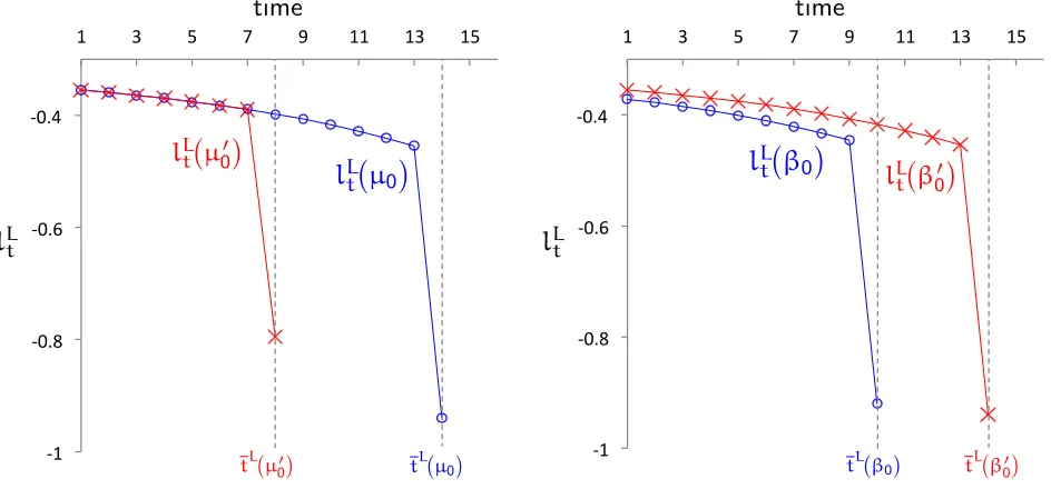
The optimal contract for the low type characterized by (6) is a penalty contract in which the magnitude of the penalty is increasing over time, with a “jump” in the contract’s final period. The jump highlights dynamic agency effects: by obtaining a success in a period t, the agent not only avoids the penaltyl_tL

but also the penaltylL_t+1 and those after. The last period’s penalty needs to compensate for the absence of future penalties. Figure 2depicts the low type’s contract; the comparative statics seen in the figure will be discussed subsequently. Only when there is no discounting does the low type’s contract reduce

to a onetime-penalty contract where a penalty is paid only if the project has not succeeded by tL. For

any discount factor, the high type’s contract characterized inTheorem 3is a onetime-penalty contract in which he only pays a penalty to the principal if there is no success by the first-best stopping timetH_{. On}

the equilibrium path, both types of the agent exert effort in every period until their respective stopping times; moreover, were the high type to take the low type’s contract (off the equilibrium path), he would also exert effort in every period of the contract. This implies that the high type gets an information rent because he would be less likely than the low type to incur any of the penalties inCL.

in the high type’s contract ofTheorem 3is chosen to be severe enough so that this contract is “too risky” for the low type to accept.

Remark1. The proof ofTheorem 3provides a simple algorithm to solve for an optimal menu of contracts.

For any_tˆ_{∈ {0, . . . , t}L_{}, we characterize an optimal menu that solves the principal’s program subject to}

an additional constraint that the low type must experiment until periodˆt. The low type’s contract in this menu is given by (6) with the termination dateˆtrather thantL. An optimal (unconstrained) menu is then obtained by maximizing the principal’s objective function overˆt_{∈ {}0, . . . , tL_}.

The characterization inTheorem 3yields the following comparative statics:

Proposition 2. AssumetH > tLand consider changes in parameters that preserve this ordering. The second-best

stopping time for typeL,tL, is weakly increasing in β0 andλL, weakly decreasing incandµ0, and can increase

or decrease inλH. The distortion in this stopping time, measured bytL−tL, is weakly increasing inµ0 and can

increase or decrease inβ0,λL,λH, andc.

Proof. See theSupplementary Appendix. Q.E.D.

Figure 2 illustrates some of the conclusions ofProposition 2. The comparative static of tL in µ0 is

intuitive: the higher the ex-ante probability of the high type, the more the principal benefits from reducing the high type’s information rent and hence the more she shortens the low type’s experimentation. Matters are more subtle for other parameters. Consider, for example, an increase inβ0. On the one hand, this

increases the social surplus from experimentation, which suggests thattLshould increase. But there are two other effects: holding fixedtL, penalties of lower magnitude can be used to incentivize effort from the low type because the project is more likely to succeed (cf. equation (6)), which has an effect of decreasing the information rent for the high type; yet, a higherβ0also has a direct effect of increasing the information

rent because the differing probability of success for the two types is only relevant when the project is good. Nevertheless,Proposition 2establishes that it is optimal to (weakly) increasetLwhenβ0increases.

Since the high type’s information rent is increasing inλH, one may expect the principal to reduce the low type’s experimentation whenλH increases. However, a higherλH means that the high type is likely to succeed earlier when deviating to the low type’s contract. For this reason, an increase inλH can reduce the incremental information-rent cost of extending the low type’s contract, to the extent that the gain in efficiency from the low type makes it optimal to increasetL.

Turning to the magnitude of distortion,tL_−tL_{: since the first-best stopping timet}L_{does not depend}

on the probability of a high type, µ0, whiletL is decreasing in this parameter, it is immediate that the

distortion is increasing in µ0. The timetLis also independent of the high type’s ability, λH; thus, since

tLmay increase or decrease inλH, the same is true fortL₋tL. Finally, with respect toβ0,λL, andc, the

!1# !0.8# !0.6# !0.4#

1# 3# 5# 7# 9# 11# 13# 15#

!1# !0.8# !0.6# !0.4#

1# 3# 5# 7# 9# 11# 13# 15#

Concluding Remarks

time H t H L t L

Low e↵ort cost, c

High e↵ort cost, c t⇤

tL(c)

tH(c)

tL(c)

tH(c)

Concluding Remarks

time H t H L t L

Low e↵ort cost, c

High e↵ort cost, c t⇤

tL(c)

tH(c)

tL(c)

tH(c)

Slide to remove

l

L_t

(

µ

0

)

l

Lt

µ

0

t

L(µ0)

t

L

(

µ0

)

l

L_t 0

l

Lt 0

t

L

₍

0

)

t

L

(

0

)

t

L

(

0

)

t

L

(

0

)

t

L

l

L_t

Slide to remove

l

L_t

(

µ

0

)

l

Lt

µ

0

t

L(µ0)

t

L

(

µ0

)

l

L_t 0

l

Lt 0

t

L

₍

0

)

t

L

(

0

)

t

L

(

0

)

t

L

(

0

)

t

L

l

L_t

To remove

t

L

µ

0

t

L

µ

00

t

L ₀0

t

L 0

l

L_t

µ

0

l

Lt

µ

00

l

L_{t 0}0

l

L_t 0

To remove

tL µ0 tLµ00

tL ₀0 tL 0

lL_t µ0 lLt µ00

lL_{t 0}0 lL_t 0

To remove

tLµ0 tLµ00 tL ₀0 tL 0

lL

t µ0 lLt µ00 lL

t 00 lLt 0 To remove

tLµ0 tLµ00 tL ₀0 tL 0

lLt µ0 lLt µ00 lL

t 00 lLt 0

To remove

tLµ0 tLµ00 tL ₀0 tL 0

lL

t µ0 lLt µ00 lL_{t 0}0 lL_t 0 To remove

tLµ0 tLµ00 tL 0

0 t

L

0

lL

t µ0 lLt µ00 lL

t 00 lLt 0

To remove

tL µ0 tL µ00

tL ₀0 tL 0

lL_t µ0 lLt µ00

lL_{t 0}0 lL_t 0

To remove

t

L

µ

0

t

L

µ

00

t

L ₀0

t

L 0

l

L_t

µ

0

l

L_t

µ

₀0

[image:19.612.73.545.57.277.2]

l

L_{t 0}0

l

L_t 0

Figure 2–The optimal penalty contract for typeLunder different values ofµ0andβ0. Both graphs

haveδ = 0.5,λL_{= 0.1,λ}H _{= 0.12, andc= 0.06. The left graph hasβ}

0 = 0.89,µ0 = 0.3, andµ00 = 0.6;

the right graph hasβ0 = 0.85,β00 = 0.89, andµ0 = 0.3. The first-best entailstL= 15on the left graph,

andtL= 12(forβ0) andtL= 15(forβ00) on the right graph.

tL₋tLwhenµ0is high; the reason is that a larger ex-ante probability of the high type makes increasing

tLmore costly in terms of information rent.

Theorem 3utilizes penalty contracts in which the agent is required to pay the principal when he fails to obtain a success. While these contracts prove analytically convenient (as explained inSubsection 5.2), a weakness is that they do not satisfyinterim participation constraints: in the implementation ofTheorem 3, the agent of either typeθwould “walk away” from his contract in any periodt_{∈ {}1, . . . , tθ_}if he could. The following result provides a remedy:

Theorem 4. AssumetH > tL. The second best can also be implemented using a menu of bonus contracts.

Specifi-cally, the principal offers typeLthe bonus contractCL= (tL, W₀L,bL)wherein for anyt_{∈ {}1, . . . , tL_},

bL_t =

tL

X

s=t

δs−t(₋l_sL), (7)

wherelLis the penalty sequence in the optimal penalty contract given inTheorem 3, andW₀Lis chosen to make the

participation constraint,(IRL), bind. For typeH, the principal can use a constant-bonus contractCH = (tH, W₀H, bH)

with a suitably chosenWH

0 andbH >0.

Generically, the above contract is the unique optimal contract for typeLwithin the class of bonus contracts. This

implementation satisfies interim participation constraints in each period for each type, i.e. each typeθ’s continuation

A proof is omitted because the proof ofProposition 1can be used to verify that each bonus contract inTheorem 4is equivalent to the corresponding penalty contract inTheorem 3, and hence the optimality of those penalty contracts implies the optimality of these bonus contracts. Using (6), it is readily verified that in the bonus sequence (7),

bL

tL=

c

βL_tLλL

andbL_t = (1−δ)c βL_tλL +δb

L

t+1for anyt∈ {1, . . . , t L

−1_}, (8)

and hence the reward for success increases over time. Whenδ = 1, the low type’s bonus contract is a constant-bonus contract, analogous to the penalty contract inTheorem 3being a onetime-penalty contract. An interpretation of the bonus contracts inTheorem 4is that the principal initially sells the project to the agent at some price (the up-front transferW0) with a commitment to buy back the output generated

by a success at time-dated future prices (the bonusesb).

5.2. Sketch of the proof

We now sketch in some detail how we prove Theorem 3. The arguments reveal how the interaction of adverse selection, dynamic moral hazard, and private learning jointly shape optimal contracts. This subsection also serves as a guide to follow the formal proof inAppendix B.

While we have defined a contract as C = (T, W0,b,l), it will be useful in this subsection alone (so

as to parallel the formal proof) to consider a larger space of contracts, where a contract is given by

C= (Γ, W0,b,l). The first element here is a set of periods,Γ⊆N\ {0}, at which the agent is not “locked out,” i.e. at which he is allowed to choose whether to work or shirk. As discussed infn. 14, this additional instrument does not yield the principal any benefit, but it will be notationally convenient in the proof. The termination date of the contract is now0 if Γ = _∅ and otherwisemax Γ. We say that a contract is

connectedifΓ =_{1, . . . , T_}for someT; in this case we refer toT as thelengthof the contract, andTis also

the termination date. The agent’s actions are denoted bya= (at)t∈Γ.

As justified byProposition 1, we solve the principal’s problem (stated at the outset of Section 4) by restricting attention to menus of penalty contracts: for each θ ∈ {L, H}, Cθ = (Γθ, W₀θ,lθ). Penalty contracts are analytically convenient to deal with the combination of adverse selection and dynamic moral hazard for reasons explained in Step 4 below.

Step 1: We simplify the principal’s program by (i) focussing on contracts for typeLthat induce him to work in every non-lockout period, i.e. on contracts in the set{CL:1∈αL(CL)}; and (ii) ignoring the constraints (IRH) and (ICLH). It is established in the proof ofTheorem 2that a solution to this simplified program also solves the original program.27 Call this program [P1].

27_{The idea for (i) is as follows: fix any contract,C}L_{, in which there is some period,t}

It is not obvious a priori what action plan the high type may use when taking the low type’s con-tract. Accordingly, we tackle a relaxed program, [RP1], that replaces (ICHL_{) in program [P1] by a relaxed}

version, called (Weak-ICHL), that only requires type H to prefer taking his contract and following an optimal action plan over taking type L’s contract and working in every period. Formally, (ICHL) re-quiresUH

0 (CH,αH(CH)) ≥U0H(CL,αH(CL))whereas (Weak-ICHL) requires onlyU0H(CH,αH(CH))≥

U₀H(CL,1). We emphasize that this restriction on typeH’s action plan under typeL’s contract is not with-out loss for an arbitrary contractCL; i.e., given an arbitraryCLwith1 _∈αL(CL), it need not be the case that1 _∈αH(CL)—it is in this sense that there is no “single-crossing property” in general. The reason is that because of their differing probabilities of success from working in future periods (conditional on the good state), the two types trade off current and future penalties differently when considering exerting ef-fort in the current period. In particular, the desire to avoid future penalties provides more of an incentive for the low type to work in the current period than the high type.28

Relaxing (ICHL) to (Weak-ICHL) is motivated by a conjecture that even though the high type may choose to work less than the low type in an arbitrary contract, this will not be the case in an optimal

contract for the low type. This relaxation is a critical step in making the program tractable because it severs the knot in the fixed point problem of optimizing over the low type’s contract while not knowing what action plan the high type would follow should he take this contract. The relaxation works because of the efficiency orderingtH > tL, as elaborated subsequently.

In the relaxed program [RP1], it is straightforward to show that (Weak-ICHL_{) and (IR}L_{) must bind at}

an optimum: otherwise, time-zero transfers in one of the two contracts can be profitably lowered with-out violating any of the constraints. Consequently, one can substitute from the binding version of these constraints to rewrite the objective function as the sum of total surplus less an information rent for the high type, as in the standard approach. We are left with a relaxed program, [RP2], which maximizes this objective function and whose only constraints are the direct moral hazard constraints (ICH

a) and (ICLa),

where typeLmust work in all periods. This program is tractable because it can be solved by separately

suboptimal for typeLto work in periodt. Since typeLwill not succeed in periodt, one can modifyCLto create a new contract,CbL_{, in whicht /}

∈bΓL_{, andl}L

t is “shifted up” by one period with an adjustment for discounting. This

ensures that the incentives for typeLin all other periods remain unchanged, and critically, that no matter what behavior would have been optimal for typeH under contractCL_{, the new contract is less attractive to typeH.}

As for (ii), we show that typeH always has an optimal action plan under contractCL _{that yields him a higher}

payoff than that of typeLunderCL_{, and hence (IR}H_{) is implied by (IC}HL_{) and (IR}L_{). Finally, we show that (IC}LH₎ can always be satisfied while still satisfying the other constraints in the principal’s program by making the high type’s contract “risky enough” to deter the low type from taking it.

28_{To substantiate this point, consider any two-period penalty contract under which it is optimal for both types}

to work in each period. It can be verified that changing the first-period penalty byε1 > 0 while simultaneously

changing the second period penalty by−ε2<0would preserve typeθ’s incentive to work in period one if and only

ifε1≤(1−λθ)δε2. Note that because−ε2<0, both types will continue to work in period two independent of their

optimizing over each type’s penalty contract. The following steps 2–5 derive an optimal contract for type

Lin program [RP2] that has useful properties.

Step 2: We show that there is an optimal penalty contract for typeLthat is connected. A rough in-tuition is as follows.29 Because typeL is required to work in all non-lockout periods, the value of the objective function in program [RP2] can be improved by removing any lockout periods in one of two ways: either by “shifting up” the sequence of effort and penalties or by terminating the contract early (suitably adjusting for discounting in either case). Shifting up the sequence of effort and penalties elimi-nates inefficient delays in typeL’s experimentation, but it also increases the rent given to typeH, because the penalties—which are more likely to be borne by type L than type H—are now paid earlier. Con-versely, terminating the contract early reduces the rent given to typeHby lowering the total penalties in the contract, but it also shortens experimentation by typeL. It turns out that either of these modifications may be beneficial to the principal, but at least one of them will be if the initial contract is not connected.

Step 3: Given any termination date TL, there are many penalty sequences that can be used by a connected penalty contract of lengthTL_{to induce the low-ability agent to work in each period1, . . . , T}L_.

We construct the unique sequence, call itl(TL), that ensures the low type’s incentive constraint for effort binds in each period of the contract, i.e. in any periodt_{∈ {}1, . . . , TL_}, the low type is indifferent between working (and then choosing any optimal effort profile in subsequent periods) and shirking (and then choosing any optimal effort profile in subsequent periods), given the past history of effort. The intuition is straightforward: in the final period, TL, there is obviously a unique such penalty as it must solve

lL_TL(TL) =−c+ (1−β

L TLλL)l

L

TL(TL). Iteratively working backward using a one-step deviation principle,

this pins down penalties in each earlier period through the (forward-looking) incentive constraint for effort in each period. Naturally, for anyTLandt_{∈ {}1, . . . , TL_},lL_t(TL)<0, i.e. as suggested by the term “penalty”, the agent pays the principal each time there is a failure.

Step 4: We show that any connected penalty contract for typeLthat solves program [RP2] must use the penalty structurelL(·)of Step 3. The idea is that any slack in the low type’s incentive constraint for effort in any period can be used to modify the contract to strictly reduce the high type’s expected payoff from taking the low type’s contract (without affecting the low type’s behavior or expected payoff), based on the high type succeeding with higher probability in every period when taking the low type’s contract.30

Although this logic is intuitive, a formal argument must deal with the challenge that modifying a transfer in any period to reduce slack in the low type’s incentive constraint for effort in that period has feedback on incentives in every prior period—the dynamic agency problem. Our focus on penalty con-tracts facilitates the analysis here because penalty concon-tracts have the property that reducing the incentive

29_{For the intuition that follows, assume that all penalties being discussed are negative transfers, i.e. transfers from}

the agent to the principal.

to exert effort in any periodtby decreasing the severity of the penalty in periodthas apositive feedback

of also reducing the incentive for effort in earlier periods, since the continuation value of reaching period

tincreases. Due to this positive feedback, we are able to show that the low type’s incentive for effort in

a given period of a connected penalty contract can be modified without affecting his incentives in any other period by solely adjusting the penalties in that period and the previous one. In particular, in an arbitrary connected penalty contractCL, if typeL’s incentive constraint is slack in some periodt, we can increaselL_t and reducelL_t−1 in a way that leaves typeL’s incentives for effort unchanged in every period

s₆= twhile still being satisfied in periodt. We then verify that this “local modification” strictly reduces the high type’s information rent.31

Step 5: In light of Steps 2–4, all optimal connected penalty contracts for typeLin program [RP2] can be found by just optimizing over the length of connected penalty contracts with the penalty structure

lL(·). By Theorem 2, the optimal length,tL, cannot be larger than the first-best stopping time: tL ≤ tL. In this step, we further establish thattL is generically unique, and that generically there is no optimal penalty contract for typeLthat is not connected.

Step 6: Let CL be the contract for type L identified in Steps 2–5.32 _{Recall that [RP1] differs from} the principal’s original program [P1] in that it imposes (Weak-ICHL) rather than (ICHL). In this step, we show that any solution to [RP1] usingCLsatisfies (ICHL) and hence is also a solution to program [P1]. Specifically, we show that αH_(CL_{) = 1, i.e. if type H were to take contract C}L_{, it would be uniquely}

optimal for him to work in all periods 1, . . . , tL. The intuition is as follows: under contract CL, type

H has a higher expected probability of success from working in any periodt _≤ tL, no matter his prior

choices of effort, than does typeL in period t given that type L has exerted effort in all prior periods (recall1_∈αL_(CL_{)). The argument relies onTheorem 2having established thatt}L _≤tL_{, becauset}H _{> t}L

then implies that for any t ∈ {1, . . . , tL}, β_tHλH > βL_tλLfor any history of effort by type H in periods

1, . . . , t−1. Using this property, we verify that because CL makes typeLindifferent between working and shirking in each period up totL(given that he has worked in all prior periods), typeHwould find it strictly optimal to work in each period up totLno matter his prior history of effort.

5.3. Implications and applications

Asymmetric information and success. Our results offer predictions on the extent of experimentation and innovation. An immediate implication concerns the effects of asymmetric information. Compare

31_{By contrast, bonuses have anegative feedback: reducing the bonus in a periodtincreases the incentive to work in}

prior periods because the continuation value of reaching periodtdecreases. Consequently, keeping incentives for effort in earlier periods unchanged after reducing the bonus in periodtwould require a “global modification” of reducing the bonus in all prior periods, not just the previous period. This makes the analysis with bonus contracts less convenient.

32_{The initial transfer inC}L_{is set to make the participation constraint for typeLbind. In the non-generic cases}