On the detection of superdiffusive behaviour in time series

warwick.ac.uk/lib-publications

Original citation:

Gottwald, Georg A. and Melbourne, Ian. (2016) On the detection of superdiffusive behaviour

in time series. Journal of Statistical Mechanics: Theory and Experiment, 2016. 123205.

Permanent WRAP URL:

http://wrap.warwick.ac.uk/84265

Copyright and reuse:

The Warwick Research Archive Portal (WRAP) makes this work by researchers of the

University of Warwick available open access under the following conditions. Copyright ©

and all moral rights to the version of the paper presented here belong to the individual

author(s) and/or other copyright owners. To the extent reasonable and practicable the

material made available in WRAP has been checked for eligibility before being made

available.

Copies of full items can be used for personal research or study, educational, or not-for-profit

purposes without prior permission or charge. Provided that the authors, title and full

bibliographic details are credited, a hyperlink and/or URL is given for the original metadata

page and the content is not changed in any way.

Publisher’s statement:

“This is an author-created, un-copyedited version of an article accepted for publication in:

Journal of Statistical Mechanics: Theory and Experiment The publisher is not responsible for

any errors or omissions in this version of the manuscript or any version derived from it. The

Version of Record is available online at :

https://doi.org/10.1088/1742-5468/aa4f0f

”

A note on versions:

The version presented here may differ from the published version or, version of record, if

you wish to cite this item you are advised to consult the publisher’s version. Please see the

‘permanent WRAP URL’ above for details on accessing the published version and note that

access may require a subscription.

series

G A Gottwald1, I Melbourne2

1 _{School of Mathematics & Statistics, The University of Sydney, Sydney 2006} NSW, Australia

2 _{Mathematics Institute, University of Warwick, Coventry CV4 7AL, United}

Kingdom

E-mail: [email protected]

E-mail: [email protected]

Abstract. We present a new method for detecting superdiffusive behaviour and for determining rates of superdiffusion in time series data. Our method applies equally to stochastic and deterministic time series data (with no prior knowledge required of the nature of the data) and relies on one realisation (ie one sample path) of the process. Linear drift effects are automatically removed without any preprocessing. We show numerical results for time series constructed from i.i.d.α-stable random variables and from deterministic weakly chaotic maps. We

compare our method with the standard method of estimating the growth rate of the mean-square displacement as well as the p-variation method, maximum

likelihood, quantile matching and linear regression of the empirical characteristic function.

Date: October 2016

1. Introduction

The ubiquity of normal diffusion can be understood by the Central Limit Theorem which, roughly speaking, states that an appropriately scaled sum of many inde-pendent identically distributed random variables with finite variance converges in distribution to a normally distributed random variable. Hence, the erratic motion of a grain of pollen suspended in water, as observed by the botanist Brown in 1827, can be understood as the relatively heavy grain experiencing the sum of many uncorrelated kicks of the chaotic much lighter water molecules. It has become evident that Brownian mo-tion and its associated normal diffusion is too simplistic to describe the variety of diffusion processes in complex systems. There are many situations where the Central Limit Theorem fails [1, 2, 3, 4, 5], and their fluctu-ations are of the so called L´evy type rather than of the Gaussian type. Whereas Gaussian processes are continuous processes with finite variance, L´evy pro-cesses (orα-stable processes) exhibit jumps of all sizes and have infinite variance. The recent survey articles [6, 7, 8, 9, 10] discuss a plethora of experimental sit-uations in which anomalous diffusion is observed and provide an overview of current analytical approaches.

Distilling the information relevant to anomalous dif-fusion, in particular determining accurately the diffu-sion rate,ns_{, presents a significant scientific challenge.} Here, s = 1₂ denotes normal diffusion and s 6= 1₂ de-notes anomalous diffusion. Of particular interest is the case of α-stable processes with superdiffusive rate

s= 1

α >

1

2. In the case ofi.i.d. data, this problem is

well-understood and various techniques such as max-imum likelihood methods [11, 12], quantile matching [13] and linear regression of the empirical characteris-tic function [14, 15] are very effective for determining

αand hences; see for example the exposition in [12]. However, these methods are not designed to deal with data that is noisy and/or non-i.i.d. In practice, the na-ture of a given time series (which may bei.i.d., noisy, or even deterministic [2, 3]) is not known in advance. Hence it is of great importance to have a method that applies to time series regardless of their origin.

One such method involves the analysis of the mean-square displacement which grows linearly for normal diffusion and sub-linearly or super-linearly for anoma-lous sub- and super-diffusion, respectively. We show

numerically that estimating the asymptotic growth rate of the mean-square displacement is not an efficient method for distinguishing anomalous from normal dif-fusion; in finite-size time series the statistical behaviour of rare large jumps is not resolved. We therefore sug-gest to use lower-order moments of orderq≪1 where the many well-resolved small jumps contribute more than the rare large jumps.

In addition it is well known that the estimation of asymptotic growth rates often suffers from a bias caused by a non-zero mean of the observables, and re-quires error prone pre-processing of the data to sub-tract the mean, or the employment of detrended fluc-tuation analysis [16, 17]. We propose a new method where an eventual non-zero mean is inherently removed by calculating theq’th moments not of the time series directly but of a related twisted time series obtained by rotating the original data with a deterministic periodic driver.

A different approach to detect anomalous diffusion is to employ thep-variation which recently found lots of ap-plication in successfully detecting anomalous behaviour in time series [18, 19, 20, 21, 22]. In this method, however, contamination of the data with additive noise has been shown to mask underlying anomalous diffu-sive behaviour as discussed in [23]. We compare our method with the standard method of estimating the asymptotic growth rate of theq’th moment as well as with the method ofp-variation and various other stan-dard methods, such as the maximum likelihood method [11, 12], quantile matching [13] and linear regression of the empirical characteristic function [14, 15], for uncon-taminated data and for data conuncon-taminated by biased additive measurement noise. We use data generated from i.i.d.random variables as well as from determin-istic weakly chaotic maps.

are presented in Section 5. We conclude in Section 6 with a summary and discussion.

2. Time series data

We will apply the tests to discrete time series

{ϕ(j)}j=1,···,N which are generated both stochastically and deterministically. To distill information about the diffusive nature of the underlying system we construct from the time series the Birkhoff sums

Φ(n) = n−1

X

j=0

ϕ(j). (1)

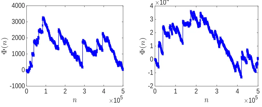
In the stochastic case, we consider i.i.d. sequences of α-stable random variables ϕ(j). Such random variables Sα(β, µ, σ) are uniquely characterized by four parameters: asymmetry parameter β, location parameterµand spread parameterσtogether withα. Numerically, we generated these random variables via the method of Chambers, Mallows and Stuck [24]. In Figure 1 we show Φ(n) for α= 1.5,β = 1, µ= 1 and

σ = 0.1. The linear drift in the Birkhoff sum Φ(n) caused by µ 6= 0 has been subtracted by computing the sample mean forα >1, i.e. by consideringϕ(j)→

ϕ(j)−(1/n)Pn_m−₌₀1 ϕ(m).

To generate the time series deterministically we employ Pomeau-Manneville intermittency maps [25]. In particular, we use the map yn+1 = f(yn) with f : [0,1]→[0,1] studied by [26]

f(y) = (

y(1 + 2z_yz_{), y∈[0,}1 2)

2y−1, y∈[1 2,1]

. (2)

This map has a neutral fixed point aty= 0. Forz= 0 the map reduces to the doubling map which preserves the uniform measure on the interval [0,1] and exhibits exponential decay of correlations. For z ∈ (0,1), there exists a unique absolutely continuous invariant ergodic probability measure, and correlations decay at the rate n−(z−1₋₁₎

[27]. Correlations are summable if and only ifz < 1₂, and in this situation the central limit theorem applies withn−1

2Φ(n) converging in law to a normal distribution for mean zero H¨older observables

ϕ [28]. For z ∈ (1₂,1), however, Gou¨ezel [3] proved that for sufficiently smooth mean zero observablesϕ(y) which are non-zero at the neutral fixed point, the central limit theorem fails and insteadn−zPn−1

j=0 ϕ(yj) converges in distribution to a stable law of exponent

α= 1/z, asymmetry β =±1 and mean µ = 0. The jumps are produced by the orbit spending prolonged times near 0 with ϕ ≈ ϕ(0). In order to get better statistics, we consider the induced map, which effectively condenses the many small jumps to a single big jump. The inducing is performed by passing from

the nonuniformly expanding map f : [0,1]→[0,1] to the uniformly expanding first return map F = fτ _: Y → Y with Y = [1/2,1] where τ(y) = inf{n ≥ 1 :

fny ∈Y} is the first return time back into the setY

fory∈Y. Induced observables are then defined as

ϕI(y) = τ(y)−1

X

ℓ=0

ϕ(fℓy), (3)

leading to Φ(n) = Pn_j=0−1ϕI ◦Fj via iteration of this procedure.

In Figure 1 we show the time series Φ(n) for

α = 1.25 generated via the map (2) with z = 0.8 for the observable ϕ(y) = 1 +y. The linear drift of the Birkhoff sum Φ(n) was again approximately elimi-nated by subtracting the sample mean.

3. Scaling behaviour of the q’th moments

We now investigate the scaling behaviour of the

q’th moment E|Φ(n)|q_{. Envoking ergodicity the q’th} moment is expressed by the time average

E|Φ(n)|q= lim N→∞

1

N N−1

X

j=0

|Φ(j+n)−Φ(j)|q . (4)

In the case of zero-mean i.i.d. α-stable random variables, the q’th moments exist for q < αand scale as

E|Φ(n)|q _∼nq

α. (5)

Forq≥αtheq’th moments do not exist. In the case of anomalous diffusion of underlying deterministic weakly chaotic dynamics, the moments exist for all values ofq

and scale as follows (

E|Φ(n)|q_∼nq/α _{q < α}

E|Φ(n)|q_≈nq+1−α _{q > α}. (6)

(We writean∼bn if there exists a constantc >0 such that limn→∞an/bn=c. We writean≈bn if there ex-ists constantsC1, C2 >0 such that C1 ≤an/bn ≤C2

for alln ≥1.) For the Brownian motion case we ob-tain the linear scaling of the mean-square displacement E|Φ(n)|2 _{∼n. Bi-linear scaling as in (6) was}

experi-mentally observed in active transport of polystyrene beads in living cells [29] and has been studied theoret-ically in infinite horizon billiards, intermittent maps and L´evy walks [30, 31, 32, 33]. For a rigorous mathe-matical proof of (6), see [34, 35].

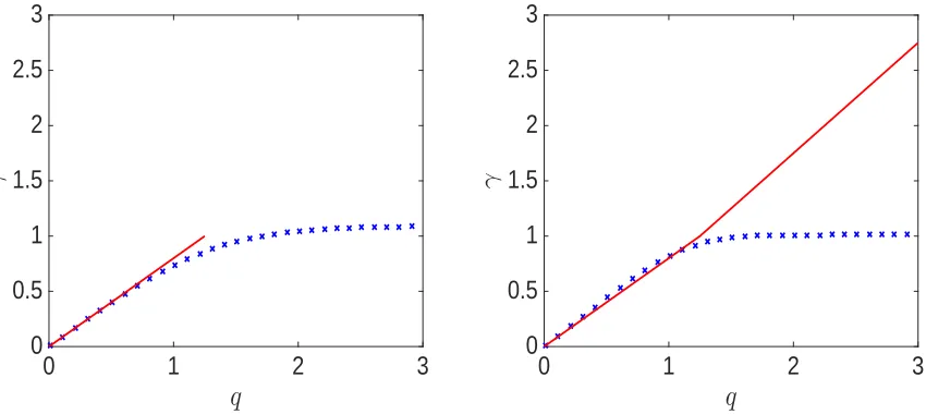
We now investigate the scaling behaviour of the

q’th moments by plotting the growth rate

γ(q) = lim n→∞

log(E|Φ(n)|q₎

n

_×

10

0

1

2

3

4

5

Φ

(

n

)

-1000

0

1000

2000

3000

4000

n

_×

10

0

1

2

3

4

5

Φ

(

n

)

×

10

-2

-1

0

1

2

3

4

Figure 1: Realization of an α-stable process Φ(n) generated from i.i.d. variables withα= 1.25, β = 1, µ= 1,

σ= 0.1 (left) and through the deterministic map (2) withz= 1/1.25 = 0.8 and observable ϕ(y) = 1 +y. The sample mean has been subtracted from the observablesϕ(j).

for several values of q for i.i.d. observables and from observables obtained from a deterministic intermittency map. To avoid any issue with a non-zero mean of the observables creating non-negligible drift terms of E|Φ(n)|q_{, we symmetrize the intermittency} map (2) and consider the map yn+1 = fsym(yn) with fsym: [−1,1]→[−1,1]

fsym(y) =

  

 

−2y, 0≤y≤1

2

1−(1−y)(1 + 2z_(1−y)z_), 1

2 ≤y≤1

−fsym(−y), −1≤y≤1

(8) with neutral fixed points aty=±1. To determine the asymptotic growth rateγ(q) from a single time series, we need to respect the double limit in the temporal average (4). The double limit requires us to choose

n≪N. In practice we usen≤N/10. The asymptotic growth rate is then determined by linear regression of

E|Φ(n)|q_.

Figure 2 shows results of numerical simulations for time series of length N = 500,000. Whereas the simulations confirm the theoretical growth rate γ(q) implied by (6) for small values of q it is clearly vio-lated for largeq > α. In particular, for the usual value

q = 2, the implied value for the anomalous diffusion is αest = 2/γ ≈2. This suggests that the estimation

of the mean-square displacement (q= 2) would falsely classify anomalous diffusion as normal with a linear growth.

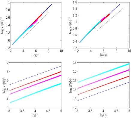
In Figure 3 we show theq’th moment as a function of

n for several values of N for q = 0.2 and q = 2 for

α= 1.25. Forq= 0.2, the convergence to the theoret-ical scaling result (5) and (6), respectively, is clearly

seen (top panel). For q = 2, the growth rate is ap-proximately equal to 1 for thei.i.d.case as well as for the Pomeau-Manneville case, consistent with the re-sults presented in Figure 2 (bottom panel). It is also clearly seen that the 2nd moments have not converged. Note that this is consistent with the nonexistence of the 2nd moment in thei.i.d. case. For the determinis-tic Pomeau-Manneville case in which the 2nd moment exists, however, this illustrates that N = 500,000 is insufficient to determine the slope of 3−α(cf (6)).

The results show that calculating the mean-square displacement is not satisfactory for distinguishing anomalous superdiffusion and normal diffusion in finite time series; note that the time series of N = 500,000 data points is rather large. The results rather suggest to use lower moments with small values ofqto estimate the anomalous coefficient α. A heuristic explanation for the superior performance of lower moments is that in a finite data set the statistics of the large jumps are necessarily not well resolved. For low values of q ≪ 1 the smaller jumps, for which better statistics are available within a finite data set, receive a relatively larger weighting than larger jumps in the time average (4). The relative importance of large jumps in the q’th moment (4) is increased for large values ofq.

4. Methods of detection

4.1. Standard estimation methods

0

1

2

3

q

0

0.5

1

1.5

2

2.5

3

γ

0

1

2

3

q

0

0.5

1

1.5

2

2.5

3

γ

Figure 2: The growth rate γ of the q’th momentE|Φ|q _∼nγ _{forφ(y) =y as a function of qfor the i.i.d. case} with µ= 0, σ= 0.1,β = 0 and α= 1.25 (left) and for the Pomeau-Manneville map (8) (right) for α= 1.25. The continuous curve (online red) depicts the theoretical result according to (5) or (6), respectively.

are not contaminated by noise. There are numerous techniques such as maximum likelihood estimators [11, 12], quantile matching [13] and linear regression of the empirical characteristic function [14, 15]. The reader is referred to [36, 12] for a detailed description and numerical comparisons in the case of pure i.i.d.

random variables. In the numerical results presented in Section 5 we use publicly available matlab routines for the quantile matching [37, 38] and for the linear regression method [38], and use the software package

STABLE [39] for the maximum-likelihood estimator‡.

4.2. Measuring the asymptotic growth rate of theq’th moment

The first method is the standard determination of the asymptotic growth rateγ of the q’th moment via linear regression for a given time series of length N. Motivated by the numerical results from the previous Section we choose q = 1/8. A non-zero mean of the observables ϕ(j) would dominate the asymptotic behaviour of the q’th moments leading to γ(q) = q, independent of the underlying diffusive nature of the dynamics. We therefore subtract the sample mean

N−1PN−1

j=0 ϕ(j) from the observables for α >1. Note

that the mean is not defined forα <1 in the case of

i.i.d.random variables (cf. Section 3). Hence, without

a prioriknowledge ofα, subtracting the sample mean is problematic.

‡ We have also used the matlab built-in commandmle[40] for

the maximum-likelihood estimator. but found it less reliable

than the commandstablefitmlefrom the STABLE package.

4.3. Measuring the asymptotic growth rate of the twisted q’th moment

To account for a possible non-zero mean of the observables ϕ(j) we consider instead of (1) the following rotated Birkhoff sum

Φc(n) = n−1

X

j=0

ϕ(j) coscj (9)

where c6= 0 is fixed. Including the rotational variable coscj assures that the mean of Φc is automatically zero. (A rigorous justification is based on [41, Section 3] via the ergodic theorem. Intuitively, the linear drift of the Birkhoff sum Φc(n) has no preferred direction in the complex plane due to the rotation variable, and hence averages to zero. The inclusion of a rotational variable has proven very useful in the detection of deterministic chaos using the 0-1 test for chaos [42, 43, 44, 45].) We will see in Section 5 that this has advantages over manually subtracting the sample mean, as in the previous Subsection, which may contaminate the statistics. We then calculate the

2

4

6

8

10

log

n

-0.2

0

0.2

0.4

0.6

0.8

1

lo

g

E

|

Φ

|

2

4

6

8

10

log

n

0.2

0.4

0.6

0.8

1

1.2

1.4

1.6

lo

g

E

|

Φ

|

3

3.5

4

4.5

5

log

n

3

4

5

6

7

8

lo

g

E

|

Φ

|

3

3.5

4

4.5

5

log

n

12

13

14

15

16

17

lo

g

E

|

Φ

|

Figure 3: The qth moment E|Φ|q _{for ϕ(y) = y for the i.i.d. case (left) and for the Pomeau-Manneville map} (8) (right). Results are shown forα = 1.25 for time series of length N = 500,000 (dashed line, online blue),

N = 100,000 (crosses, online red), N = 50,000 (open circles, online magenta) and N = 25,000 (diamonds, online cyan). Top: Forq = 0.2 < α. Bottom: For q = 2> α. The dashed lines in the top figures show the theoretical slope as calculated via (5) and (6), respectively. The slope in the bottom figures is approximately 1 (cf. Figure 2).

than the mean to avoid the effect of outliers. In practice we find that 100 randomly chosen values of

c∈(π/5,4π/5) are sufficient.

4.4. p-variation method

Thep-variation associated with a process Φ is defined as the asymptotic limit

Vp(t) = lim n→∞V

n

p(t), (10)

where Vn

p(t) is the partial sum of increments of the observable Φ(n) given by

Vpn(t) = ⌊nt⌋ X k=1 Φ k n

−Φk−1

n p .

For p = 1, V1(t) reduces to the total variation, and

for p = 2, V2(t) reduces to the quadratic variation.

It is known that for Brownian motion, V2(t)∼ t and Vp(t) = 0 for anyp >2. In the case of subdiffusion, the p-variation allows to distinguish fractional Brownian motion and Continuous Time Random Walk (CTRW) diffusion [18, 20]. For fractional Brownian motion,

V2(t) is a monotonically increasing step function and V2/γ⋆(t) = 0, where γ⋆ = γ(2) is the asymptotic

growth rate of the mean-square displacement. For superdiffusion, Vpn(t) converges for p > α and diverges for p < α for n → ∞. This suggests to estimate α by determining the smallest value p⋆ _for which convergence occurs and set αest = p⋆. In

practice, we subsample a time series of length N

into 2m _{data points with equal spacing N/2}m _with m = 0,· · · ,⌊logN/log 2⌋. For the finest samplings we estimate a linear approximation ˆVn

p (t) by linear regression of Vn

p(t). We determine p⋆ then as the minimal value of p for which the ℓ1-norm of the

difference between two consecutive samplings|Vˆn p (t)− ˆ

Vn−1

p (t)| falls below some thresholdθp. The choice of the thresholdθpis, of course, arbitrary and depends on the underlying dynamical system which is analyzed.

4.5. Modifiedp-variation method

In [46, 21] theorems were proved showing that for an α-stable random variable with location parameter

µ = 0 and α = p/2 (and any values of β and

σ) its p-variation Vn

p (t) converges in distribution to an α = 1/2-stable random variable S1/2(1,0, σ) with

some specified spread parameter σ. In [21] this was developed into a time series analysis method using a Kolmogorov-Smirnov test and finding the value of

p= 2αfor which the empirical cumulative distribution function is closest to the target cumulative distribution function of S1/2(1,0, σ). To estimate the cumulative

distribution function of Vn

p(t), an ensemble of p -variations is generated by segmenting the time series into M pieces, each being ⌊N/M⌋ long. This tacitly assumes that the samples are uncorrelated which is only approximately true for sufficiently long segments in the deterministic case. The minimal Kolmogorov-Smirnov distance is determined by varying the spread parameterσof the target distribution S1/2(1,0, σ) for

each value ofp. The value p⋆ _{for which the minimum} is attained then determines α = p⋆_{/2. The precise} mathematical statement is provided in Appendix A. For details on the modified p-variation method see [46, 21].

5. Numerical results

We use a time series of length N = 25,000 calculated from i.i.d. random variables and from weakly chaotic deterministic variables. We show results for pure data and for noise-contaminated data. To calculate theq’th momentsE|Φ|q _{we employq= 1/8. For thep-variation} method we use θp = 0.01 and cycle through p in increments of ∆p= 0.005. We found that larger values of θp perform better for larger values of α but worse for smaller values of α. For the modified p-variation

method, we choose M = 250 samples of length 100 each, and cycle through 10,000 values of the spread parameterσ∈(10−2,1010) (equidistant in log-space).

5.1. Results for the i.i.d.case

We use a time series of lengthN = 25,000 constructed by the Chambers, Mallows and Stuck [24] method. We set the asymmetry parameter β = 1 and the spread parameter σ = 0.1, and allow for a non-zero mean parameterµ= 2.

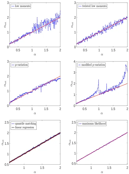
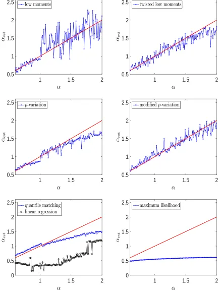
In Figure 4 we show results for the estimated value ofαfor the methods described in the previous Section. For the methods using the asymptotic growth rate γ

we estimate the implied value forαest=q/γ forα > q.

The method of estimatingαvia the asymptotic growth rate of theq’th moment for lowqperforms very well for

α <1, but has large errors forα >1. This is due to the non-accuracy in determining the mean via the sample mean which is subtracted forα >1. This undesirable property is alleviated when estimating the asymptotic growth rate of the twistedq’th moment, whereαis well estimated for the whole range of α. The standard p -variation performs well except nearα= 1 andα= 2. It is more accurate than the twisted low moment method for 1< α < 1.5. The modifiedp-variation has strong difficulties in estimating the anomalous diffusion near

α = 1 and α > 1.75. We have tested that the bad performance of the modified p-variation method near

α = 1 is due to the non-vanishing mean parameter

µ= 2 and the asymmetryβ= 1. Forµ= 0 andβ = 0 (and all other parameters unchanged), the modifiedp -variation method performs well near α= 1. The bad performance near the Brownian case α = 2 remains though for µ= 0 andβ = 0. As expected, the meth-ods described in Section 4.1 perform best in the case of noise-less i.i.d. random variables. The methods of quantile matching, linear regression of the empirical characteristic function and, in particular, the maxi-mum likelihood estimator very accurately estimate α

for the whole range ofα.

We also present results where we contaminate the observationsϕ(n) by biased uniform noise according to

0.5

1

1.5

2

0

1

2

3

0.5

1

1.5

2

0

1

2

3

0.5

1

1.5

2

0

1

2

3

0.5

1

1.5

2

0

1

2

3

4

1

1.5

2

0.5

1

1.5

2

2.5

1

1.5

2

0.5

1

1.5

2

2.5

Figure 4: Estimatesαest as calculated for several values α∈ (0.2,2) fori.i.d. observations. Top left: method

of lowq’th moment with q = 1/8. Top right: method of twisted lowq’th moment with q = 1/8. Middle left:

methods are not able to reliably estimate the stable parameterα when the data is contaminated by noise as shown in the bottom row of Figure 5.

5.2. Results for the Pomeau-Manneville case

We use a time series of lengthN = 25,000 constructed from the Pomeau-Manneville map (2) forα∈(0.6,2). We chooseϕ(n) = 1+xn. Figure 6 shows the analogous results to Figure 4.

In the deterministic case, we observe the same be-haviour of low moments as in the i.i.d. case where anomalous diffusion is very well classified for α < 1 but not so well forα >1 where the error in estimating the sample mean has a detrimental effect. The twisted low moment method performs well, except near the Brownian case of α = 2 where it underestimates the anomalous scaling coefficient. The slow convergence may be related to cross-correlation effects that arise in the diffusion parameter via the Green-Kubo formula. Such cross-correlations are not present in the superdif-fusive case α < 2 [3]. The p-variation also does not perform well. Near α = 1 and the Brownian case

α= 2 thep-variation strongly flattens and underesti-mates the anomalous scaling coefficient. The modified

p-variation, in contrast, performs well for the whole range ofα. As in the case of noisyi.i.d. variables, the standard i.i.d. estimation methods described in Sec-tion 4.1 do not reliably estimate the stable parameter

α for the whole range of α. Curiously, the quantile matching method performs well forα <1.

Again, we also present results for observations which have been contaminated with biased uniform noise with η = 0.5 in Figure 7. As in the i.i.d.

case, the performance of the low moment method and the p-variation method is diminished by the additive measurement noise. The performance of the twisted low moment method and the modified p-variation method, however, are robust against additive measure-ment noise. The standardi.i.d.estimation methods de-scribed in Section 4.1 fail reliably estimate the stable parameterαfor the whole range ofα. Again, the quan-tile matching method performs well for α < 1. The method of linear regression of the empirical charac-teristic function and the maximum likelihood method significantly underestimate the value ofα.

6. Summary and Discussion

We have introduced a new method to quantitatively estimate the degree of anomalous superdiffusion. Our method uses the asymptotic growth rate of a twisted low moment derived from the data rotated with a pe-riodic deterministic signal.

We established that the standard method of estimat-ing the growth-rate of the mean-square displacement is not able to reliably distinguish superdiffusion from nor-mal diffusion in finite time series. We have compared our method then with ive other methods, a method based on (untwisted) low moments, two versions of the

p-variation method as well as the standard estimators analysing the empirical characteristic function and es-timating the maximum likelihood developed for i.i.d.

random variables.

Whereas the standard methods such as quantile match-ing, linear regression of the empirical characteristic functionand maximum likelihood estimatorsare by far superior in estimating the stable parameter α in the case of noise-free i.i.d. random variables, they fail in the case of noisyi.i.d. random variables and/or deter-ministically generated variables. Our numerical simu-lations on noisyi.i.d. data and data generated deter-ministically from weakly chaotic Pomeau-Mannneville maps, reveal that our new method and the modified

p-variation as proposed in [21] perform best and are most robust to additive measurement noise, which is in-evitable in any real-world application. The modifiedp -variation and our newly proposed twisted low moment method have been shown to have complementary ad-vantages. Whereas the modified p-variation performs very well in the case of deterministic data, it did less so for the i.i.d.case, in particular for values ofαnear 1 and 2. In contrast, our new method performs well in the case ofi.i.d.random variables, but becomes less accurate in the deterministic case for values of α ap-proaching Brownian diffusion withα= 2. We therefore propose our method to be used in conjunction with the

p-variation to gain further insights into the quantita-tive analysis of anomalous diffusion from time series. The computational cost involved in applying those methods varies significantly. The standardp-variation method and the method of estimating the asymptotic growth rate of a low moment are the least computa-tionally demanding methods. For the twisted low mo-ments, one needs to cycle over typically 100 different values of the frequency c of the periodic signal. The modified p-variation method requires cycling through values of σ, which requires tuning over a large range of values. Despite the variation in the computational cost of the methods, all the methods use only a single sample time series.

Acknowledgments

We would like to thank John Nolan for generously

sharing his software package STABLE with us. This

0.5

1

1.5

2

0

1

2

3

0.5

1

1.5

2

0

1

2

3

0.5

1

1.5

2

0

1

2

3

0.5

1

1.5

2

0

1

2

3

4

1

1.5

2

0.5

1

1.5

2

2.5

1

1.5

2

0.5

1

1.5

2

2.5

Figure 5: Estimates αest as calculated for several values α ∈ (0.2,2) for i.i.d. observations with 50% biased

1

1.5

2

0.5

1

1.5

2

2.5

1

1.5

2

0.5

1

1.5

2

2.5

1

1.5

2

0.5

1

1.5

2

2.5

1

1.5

2

0.5

1

1.5

2

2.5

1

1.5

2

0

0.5

1

1.5

2

2.5

1

1.5

2

0

0.5

1

1.5

2

2.5

Figure 6: Estimates αest as calculated for several values α∈(0.6,2) for the Pomeau-Manneville map (2). Top

1

1.5

2

0.5

1

1.5

2

2.5

1

1.5

2

0.5

1

1.5

2

2.5

1

1.5

2

0.5

1

1.5

2

2.5

1

1.5

2

0.5

1

1.5

2

2.5

1

1.5

2

0

0.5

1

1.5

2

2.5

1

1.5

2

0

0.5

1

1.5

2

2.5

Figure 7: Estimatesαest as calculated for several values α∈(0.6,2) for the Pomeau-Manneville map (2) with

a European Advanced Grant StochExtHomog (ERC AdG 320977).

Appendix A. Modifiedp-variation

We recall here Theorem 2.1 from [21]

Theorem 1 For an α-stable process Xt with Xt ∼ Sα(β,0, σ), we have for p > α/2 that its p-variation Vn

p (t)converges in the Skorohod topology with Vpn(t)−ntBn(α, p)−→D Xt′ as n→ ∞,

whereX′ t∼Sα

p(1,0, σ

′_{) with spread parameter}

σ′ =  



σpcos(πα2p)Γ(1− α

p)

cos(πα

2p)Γ(1−α)

p/α

α6=p

σ α=p

, (A.1)

and normalising sequence

Bn(α, p) =   

 

n−p/α_E|X|p _{p∈(α/2, α)} Esin n−1_|X|α

α=p

0 p > α

. (A.2)

References

[1] Klafter J, Shlesinger M and Zumofen G 1996Physics Today

4933

[2] Gaspard P and Wang X J 1988Proceedings of the National Academy of Sciences85_4591–4595

[3] Gou¨ezel S 2004Probability Theory and Related Fields128

82–122

[4] Cont R and Tankov P 2004Financial modelling with jump processesChapman & Hall/CRC Financial Mathematics Series (Chapman & Hall/CRC, Boca Raton, FL) ISBN 1-5848-8413-4

[5] Mantegna R N and Stanley H E 2007 An introduction to econophysics: Correlations and complexity in finance (Cambridge University Press, Cambridge) ISBN 978-0-521-03987-1; 0-521-03987-8

[6] Metzler R and Klafter J 2000Physics Reports 339_1–77

[7] Sokolov I M 2012Soft Matter8(35) 9043–9052

[8] H¨ofling F and Franosch T 2013 Reports on Progress in Physics76046602

[9] Metzler R, Jeon J H, Cherstvy A G and Barkai E 2014 Phys. Chem. Chem. Phys.16_{(44) 24128–24164}

[10] Metzler R, Jeon J H and Cherstvy A 2016Biochimica et Biophysica Acta (BBA) - Biomembranes 18582451 – 2467 ISSN 0005-2736 biosimulations of lipid membranes coupled to experiments

[11] DuMouchel W H 1973Ann. Statist.1_{948–957 ISSN}

0090-5364

[12] Nolan J P 2001 Maximum likelihood estimation and diagnostics for stable distributions L´evy processes (Birkh¨auser Boston, Boston, MA) pp 379–400

[13] McCulloch J H 1986 Comm. Statist. B—Simulation Comput.15_{1109–1136 ISSN 0361-0918}

[14] Koutrouvelis I A 1980J. Amer. Statist. Assoc.75918–928 ISSN 0003-1291

[15] Koutrouvelis I A 1981 Comm. Statist. B—Simulation Comput.10_{17–28 ISSN 0361-0918}

[16] Peng C K, Buldyrev S V, Havlin S, Simons M, Stanley H E and Goldberger A L 1994Phys. Rev. E49(2) 1685–1689

[17] Peng C K, Havlin S, Stanley H E and Goldberger A L 1995 Chaos 582–87

[18] Magdziarz M, Weron A, Burnecki K and Klafter J 2009 Phys. Rev. Lett.103_{(18) 180602}

[19] Burnecki K and Weron A 2010

Phys. Rev. E 82(2) 021130 URL

http://link.aps.org/doi/10.1103/PhysRevE.82.021130

[20] Magdziarz M and Klafter J 2010Phys. Rev. E82(1) 011129 [21] Hein C, Imkeller P and Pavlyukevich I 2009 Limit theorems forp-variations of solutions of SDEs driven by additive

stable L´evy noise and model selection for paleo-climatic data Recent Development in Stochastic Dynamics and Stochastic Analysis (Interdisciplinary Math. Sciences vol 8) ed Duan J, Luo S and Wang C (World Scientific, Singapore) pp 137–150

[22] Burnecki K, Kepten E, Janczura J, Bronshtein I, Garini Y and Weron A 2012Biophysical Journal1031839–1847 [23] Jeon J H, Barkai E and Metzler R 2013 The Journal of

Chemical Physics 139₁₂₁₉₁₆

[24] Chambers J M, Mallows C L and Stuck B W 1976Journal of the American Statistical Association 71pp. 340–344 [25] Pomeau Y and Manneville P 1980Comm. Math. Phys.74

189–197

[26] Liverani C, Saussol B and Vaienti S 1999 Ergodic Theory Dynam. Systems 19_671–685

[27] Hu H 2004Ergodic Theory Dynam. Systems24_495–524

[28] Young L S 1999Israel Journal of Mathematics110153–188 ISSN 0021-2172

[29] Gal N and Weihs D 2010Phys. Rev. E 81_{(2) 020903}

[30] Armstead D N, Hunt B R and Ott E 2003 Phys. Rev. E

67_{(2) 021110}

[31] Courbage M, Edelman M, Fathi S M S and Zaslavsky G M 2008Phys. Rev. E 77(3) 036203

[32] Artuso R and Cristadoro G 2003 Phys. Rev. Lett.90(24) 244101

[33] Rebenshtok A, Denisov S, H¨anggi P and Barkai E 2014 Phys. Rev. Lett.112(11) 110601

[34] Gou¨ezel S and Melbourne I 2014Electron. J. Probab. 19

no. 93, 30 ISSN 1083-6489

[35] Dedecker J and Merlev`ede F 2015Stochastic Process. Appl.

125_{3401–3429 ISSN 0304-4149}

[36] Weron R 1995 Performance of the estima-tors of stable law parameters HSC Research Reports HSC/95/01 Hugo Steinhaus Cen-ter, Wroclaw University of Technology URL

http://EconPapers.repec.org/RePEc:wuu:wpaper:hsc9501

[37] Borak S and Weron R 2010 STABLECULL: MATLAB func-tion to estimate stable distribufunc-tion parameters using the quantile method of McCulloch Statistical Software Com-ponents, Boston College Department of Economics URL

https://ideas.repec.org/c/boc/bocode/m429006.html

[38] Veillette M 2012–2015 Stbl: Alpha

stable distributions for MATLAB

https://au.mathworks.com/matlabcentral/fileexchange/37514-stbl-[39] RobustAnalysis Nolan J P 2016

STA-BLE www.RobustAnalysis.com URL

http://www.RobustAnalysis.com

[40] MATLAB 2016 version 9.1.0 (R2016b) (Natick, Mas-sachusetts: The MathWorks Inc.)

[41] Nicol M, Melbourne I and Ashwin P 2001Nonlinearity14

275–300

[42] Gottwald G A and Melbourne I 2004Proc. Roy. Soc. A460

603–611

[43] Gottwald G A and Melbourne I 2005Physica D212100– 110

[44] Gottwald G A and Melbourne I 2009Nonlinearity22_1367–

1382

[45] Gottwald G A and Melbourne I 2009SIAM J. Appl. Dyn.

8129–145