ISSN: 1816-949X
© Medwell Journals, 2020
The Improved Differential Evolution Algorithm for Multi-Floor
Facility Layout Problems
1
Jittraporn Palakawong Na Ayutthaya,
1Nuchsara Kriengkorakot Preecha Kriengkorakot and
2Prasert Sriboonchandr
1
Department of Industrial Engineering, Faculty of Engineering, Ubon Ratchathani University,
34190 Ubon Ratchathani, Thailand
2
Department of Industrial Engineering, Faculty of Industrial Technology and Management,
Prachinburi Campus, King Mongkut’s University of Technology North Bangkok, Thailand
Abstract: This research aimed to study the Improved Differential Evolution (IDE) for solving the Multi-floor Facility Layout Problem (MFLP) with the target of minimize the transporting material costand maximize adjacency requirement between the facilities. The IDE algorithm had been evaluated and compared with MULTIPLE, SABLE and the basic DE algorithm by using DE/rand/1/bin and DE/rand/2/bin. For MFLP, the IDE methods were tested with 6 data sets as following: 11-1, 11-2, 12, 21-1, 21-2, 21-3 which found that IDE able to find the optimal solution better than the multiple is 52.67, 14.02, 15.89, 32.10, 20.01 and 36.92% for problems11-1, 11-2, 12, 21-1, 21-2 and 21-3, respectively and can generate the optimal solution that is better than the sable is 6.75, 15.85, 2.76 and 27.56% for problems 11-1, 21-1, 21-2 and 21-3, respectively. The result showed that the further performed IDE were effective methods comparing to the other algorithms and other metaheuristic methods. Hence, they could be used to solve MFLP.
Key words: Multi-floor facility layout, differential evolution, improved differential evolution, DE
INTRODUCTION
Nowadays, increasing business competition, higher economic and social growth causing the limited use of natural resources for maximum benefits, especially, high-priced land. The good location is high price. The higher price of land causing most business owners in both manufacturing and service industries to use the land worth while resulting in more vertical expansion building. Many buildings are built on multiple floors. The facility layout of multi-floor buildings is agenerally NP-hard problem which are complicated to solve and it is important to help the organization can increase efficiency and reduce material transportation cost to increase competitiveness. Researches have shown that an efficient facility can reduce manufacturing cost by 10-30% (Tompkins et al., 2010) and more than 35% of the system efficiency is likely to be lost by applying incorrect layout and locate design (Huang et al., 2010). In the addition, between 20 and 50% of operating expenses in manufacturing can be attributed to facility planning and material handling (Singh and Sharma, 2006). The effective facility layout can lead the enterprises to the well competitive in the market and make more benefits to the organization.
The researchers have used many methods to solve problems, various algorithms were create for solve the facility layout problems such as CRAFT, ALDEP and CORELAP and develop the algorithms for solving the multi floor facility layout such as SPACECRAFT, MULTIPLE, SABLE, STAGE, etc. Moreover, using mathematics with exact methods (Patsiatzis and Papageorgiou, 2002; Afrazeh et al., 2010) for finding the optimal solutions, spent more time for calculation with more variables and limitations. The optimal solution is not easy to reaching, therefore, many heuristic approacheshave been developed to get the near-optimal solutions such as simulated annealing (Meller and Bozer, 1996; Xiaoning and Weina, 2011) Genetic algorithms (Kochhar, 1998 ; Kochhar and Heragu, 1999; Lee et al., 2005), Tabu search (Abdinnour-Helm and Hadley, 2000). But not found yet the differential evolution algorithm used to solve the MFLPwith multi objective, so in this research will present the DE method for solving the MFLPs with the objectivesare minimize the transporting material costand maximize adjacency requirement between the facility.
This research is a study on Multi-floor Facility Layout Problems (MFLPs) which is a discrete layout and finding the solution by using an improved the Differential
Evolution algorithm (DE) where the objectivesare the minimization of the transporting material cost and maximize adjacency requirement between the facility. The aim of this new method is to generate the good solutions or the optimal solutions to this problem. Literature review
Multi-floor facility layout problems: The first method multi-floor facility layout (no more than 3 floors) was ALDEP which created by Seehof JM and Evans WO (Seehof and Evans, 1967). The concept of ALDEP is to try to create alternatives of the layout, start placing by sweeping from the top left corner of the layout down and consider the relationship. Johnson, RV (Johnson, 1982) offered SPACECRAFT, the algorithm developed and improved from CRAFT (Armour and Buffa, 1963) for multi-floor layout by adding the necessary import information calculation of the cost and time of moving between the floors. SPACECRAFT is aimed to minimize the material handling. Meller (1992) presents multiple as the only objective heuristic improvement that uses spacefilling curve to help create and improve layouts. Meller (1992 presents SABLE using spacefilling curve and Simulating Annealing (SA) in the layout improvement by developing to improve the efficiency of multiple. Matsuzaki et al. (1999) introduced the MUSE (Multi-Story layout) using SA (Simulated Annealing) as the basis for allocating the facility into each floor and use the GA (Genetic Algorithm) to find the number of elevators and the appropriate location for installation the elevator by considering the elevator utilization. Lee et al. (2005) presented the application of GA to solve the multi-floor facility layout problem that considers the passage which minimize total cost of materials transportation and maximization the adjacency requirement between departments. Krishnan et al. (2009) develop MIP to solve the problem of 2 floors facility layout with unequal area. The objectives are the minimization the material handling costs and the maximization the close rates.
Differential evolution algorithm for solving other problems: Differential Evolution (DE) is a method of evolution using the difference to find the optimal solution which was presented by Storn and Price in 1997. It is a popular method to solve problems in various fields such
as supply chain management problem in particular, the Vehicle Routing Problem (VRP). Xu and Wen (2012 ) employed DE to the unidirectional logistics distribution vehicle routing problem with no time widows resulting in the shortage total distance. Scheduling problem, Shahnazari-Shahrezaei et al. (2012) present DE to generate the fair shift Nurse Scheduling problem base on a real case study. Zhang et al. (2013) adapted DE method dealing with the job shop problem in order to minimize total tardiness. In the line balancing problems, (Sresracoo et al., 2018) presented the DE algorithm for solving the U-shaped Assembly Line Balancing Problem Type 1 (UALBP-1) with the goal was minimize the number of workstations. For further applying DE on other problems, electric power system, El Ela et al. (2010) use the DE method for the soultion to optimal power flow resulting in voltage stability enhancement and minimize cost. Kuila and Jana (2014) present DE for wireless sensor network system was proposed to prolong the lifetime of the system prevented from overloading.
MATERIALS AND METHODS
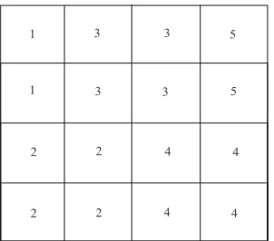
The mathematical model of the multi-floor facility layout problem: Mathematical model of the MFLP was focused on in this study and the details of the problem are as follows: the MFLP layout problem pattern: it divides the plant site into many rectangular blocks call them template, each template has the same area and shape and each template is assigned to a facility. If the facilities have unequal areas, they could occupy templates and modeled into a cell. Figure 1 which is the example of 5 facilities with 16 templates. If the facilities have equal areas, the problem likes QAP Fig. 2. The arrangement by sweeping is to be applied in to the locate department. Measuring distance between each department will be measured in rectilinear from the centroid.
Indices, notation and parameter:
Where:
i : Denotes the index of a facility i : 1, 2, 3, …, N
1 3 3 5
1 3 3 5
2 2 4 4
2 2 4 4
4 5
3 6 11 14
2 7 10 15
1 8 9 16
[image:3.612.113.264.137.270.2]13 12
[image:3.612.108.254.306.437.2]Fig. 1: The example of 5 facilities with 16 templates
Fig. 2: The example of QAP 16 facilities
I : Denotes the index of a location of template where l = 1, 2, 3,…, L
k : Denotes the index for floor k : 1, 2, 3, … , K
bi, j : Denotes the adjacency factor between
facility i and j bi, j : 0.2, 0.4, 0.6, 0.8, 1.0
Ci j : Denotes the adjacency value between i and j
Cij : 0, 1, 2, 3, 4, 5
C : Denotes maximum adjacency rating ( = 5) W1 : Denotes weight factor of material transportation
cost
W2 : Denotes Weight factor of the adjacency
di, j : Denotes the total vertical and horizontal distance
between facility i and j
: Denotes the vertical distance between facility
v ij
d
i and j
: Denotes the horizontal distance between
h ij
d
facility i and j
dmax : Denotes maximum distance between the
facilities
Cv : Denotes the vertical material transportation
Cost per unit
Ch : Denotes the horizontal material
transportation cost per unit denote the total templates
A : Denote the total templates of facility fij : Denote the material flow between facility i
and j
: Denote the distance between facility i and j with elevator 1
: Denote the distance between facility i and j
e2 i j
d
with elevator 2
xi, yi : Denote the coordinator of the centroid of
facility i
xe1, ye1 : Denote the coordinator of the elevator 1
xe2, ye2 : Denote the coordinator of the elevator 2
Zi : Denote the floor No. of the facility
H : Denote the Height between floors Decision variable:
(1)
i,l,k
1if facilityi assigned to location l and floor No.k 0 otherwise
U
(2)
i k
1if facilityiassigned to floor No.k Z
0 otherwise
(3)
i j
1if facility i assigned to thesamefloor with z
thefacility j 0otherwise
(4)
N-1 N h
1 i 1 j i 1 ij ij h ij
N-1 N
2 i 1 j i 1 ij ij
W f C d +C d +
Min
W C- b C
Subject to: (5) N ii 1aA, i
(6)
i j i j ij
h
ij e1 e2
ij ij ij
x -x + y -y ;z 1 d
Min d ,d ;z 0
(7) e1
ij i e1 i e1 j e1 j e1
d x -x + y -y + x -x + y -y
(8)
e2
ij i e2 i e2 j e2 j e2
d x -x + y -y + x -x + y -y
(9)
v
ij j i
d H z z
(10)
h v
ij ij ij
d d d
(11)
max ij
d Max d
(12) max ij max max ij max max ij ij max max ij max max ij max ij max d 1.0if 0 d
6 d d 0.8if d 6 3 d d 0.6if d 3 2 b d 2d 0.4if d 2 3 2d 5d 0.2if d 3 6 5d
0.0if d d
6 Constraints: (13) total
A A
(14)
K L
ilk i
k 1 l 1U a , i
(15)
N L K
ilk total
i 1 l 1 k 1U A
(16)
K
k 1Zik1, i
(17)
N
i k
n 1a Zik A , k
Equation 4 represent an objective function of the model to minimize the material transporting cost and maximize adjacency requirement between the facilities. Equation 5 is ensure that total templates are enough for all facilities. Equation 6 is the calculation of horizontal distances between facility i to j. Equation 7-8 is the calculation of horizontal distances between facility i to j using elevator No. 1 and 2, respectively. Equation 9 is the calculation of vertical distances between facility i to j. Equations 10 is the total distance between the facility i to j.
Equation 11 is finding the maximum distance between the facilities. Equation 12 is the adjacency factor which represents the adjacency ratio between i and j Eq. 13 is ensure that the total space is enough for all facility. Equation 14 is ensures that a plan for all facilities according to the requirement areas of each facility. Equation 15 is a restriction to prevent redundant use of the facility’s area. Equation 16 is restrictions to prevent having the same facility on separate floors. Finally, Eq. 17 is the limitation of the use of space in each floor.
The adjacency value (Cij) between facilities is a
functional relationship which not always quantifiable and it sometimes vague and difficult to define, the optimization result can vary depending on this value. Lee et al. (2005) However, in this study the adjacency propose by Lee et al. (2005) is used as shown:
Where:
Cij = 0 : It is undesirable for facilities i and j to be
located close together
Cij = 1 : It is unimportant for facilities i and j to be
located close together
Cij = 2 : It is ordinary for facilities i and j to be located
Start
Initial vector
Mutation
Crossover or recombination
Fitness evaluation
Selection
Loop repeat
Optimal result
End No
Yes Cij = 3 : It is important for facilities i and j to be located
close together
Cij = 4 : It is especially, important for facilities i and j to
be located close together and
Cij = 5 : It is absolutely necessary for facilities i and j to
be located close together
The weight factors W1 and W2 are equivalent to the
tradeoff between the total cost of transporting materials and the adjacency requirement. Therefore, the ratio of W1
and W2 can vary the optimization result. In this study, the
values W1 for W2 and are 0.5.
RESULTS AND DISCUSSION
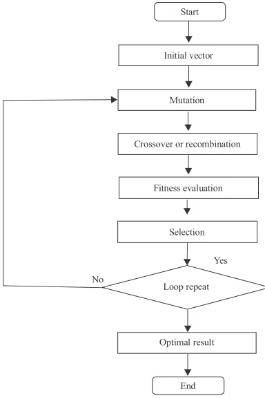
The differential evolution algorithm: The procedures of differential evolution algorithm consist of several steps: create a set of initial vectors, perform a mutation process, crossover or recombination process, fitness evaluation process and selection process. The procedure application is shown in Fig. 3.
Procedure of MFLP by using differential evolution algorithm: The procedure of MFLP uses the DE algorithm. The values used in the calculation must be set. The variable are as follows: G = Round, NP = Numbers of Population, F = Scaling factor and CR = Crossover Rate. In this example calculation, these variables were set as NP = 5, F = 2 and CR = 0.8.
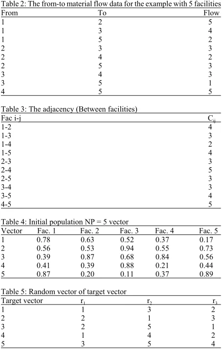
Calculation using the DE/rand/1/bin: For example, the problem is two floors with 5 facilities which have the requirement areas in Table 1, the template size is 1 square distance unit and the inter-floor distance is 5.0 distance units, material transportation horizontal cost and vertical cost are $1 and $5 per unit per distance, respectively. The material flow data and the adjacency between facilities are in the Table 1-3, respectively.
Initial population with a randomized real number between 0 and 1 for each facility (Table 4) which will be used further in mutation and crossover.
Mutation, in this step, a position of the vector is randomized (Table 5) and mutated to obtain new solutions that differ from the initial population number by targeting the mutation. The calculation for the mutant Vector (Vi, j, G) is shown in Eq. 18 and an example of a
[image:5.612.333.525.136.425.2]mutation is illustrated in Table 5:
Fig. 3: The DE algorithm procedure
Table 1: Requirement area
Variables Area
Fac.1 4
Fac.2 4
Fac.3 8
Fac.4 8
Fac.5 8
(18)
i, j, G r3,G r1,G r2,G
V X +F X -X
Where:
Vi, j, G : Mutant Vector
Xr1G, Xr2, G, : Random vector
Xr3, G
4
4
4
4 4
4
4
4 5
5
5
5 5
5
5
5
2
2
2
2 3
3
3 3
3
3
3 1
1
1
1
Elevator
[image:6.612.71.298.138.500.2]Floor 1 Floor 2
Table 2: The from-to material flow data for the example with 5 facilities
From To Flow
1 2 5
1 3 4
1 5 2
2 3 3
2 4 2
2 5 3
3 4 3
3 5 1
4 5 5
Table 3: The adjacency (Between facilities)
Fac i-j Cij
1-2 4
1-3 3
1-4 2
1-5 4
2-3 3
2-4 5
2-5 3
3-4 3
3-5 4
4-5 5
Table 4: Initial population NP = 5 vector
Vector Fac. 1 Fac. 2 Fac. 3 Fac. 4 Fac. 5
1 0.78 0.63 0.52 0.37 0.17
2 0.56 0.53 0.94 0.55 0.73
3 0.39 0.87 0.68 0.84 0.56
4 0.41 0.39 0.88 0.21 0.44
5 0.87 0.20 0.11 0.37 0.89
Table 5: Random vector of target vector
Target vector r1 r2 r3
1 1 3 2
2 2 1 3
3 2 5 1
4 1 4 2
5 3 5 4
Table 6: Results of mutation in target vector 1 by using DE/rand/1 (F = 2)
Facility 1 2 3 4 5
Xr1 = Vector 1 (1) 0.78 0.63 0.52 0.37 0.17 Xr2 = Vector 3 (2) 0.39 0.87 0.68 0.84 0.56 Xr3 = Vector 2 (3) 0.56 0.53 0.94 0.55 0.73 (1)-(2) (4) 0.39 -0.24 -0.16 -0.47 -0.39 Fx(4):2x (4) (5) 0.78 -0.48 -0.32 -0.94 -0.78 Mutant vector:(3)+(5) 1.34 0.05 0.62 -0.39 -0.05
Table 7: Results of binomial crossover in vector 1 by DE/rand/1/bin (CR = 0.8)
Facility 1 2 3 4 5
Randb (j) 0.50 0.69 0.98 0.19 0.47
Target vector 0.78 0.63 0.52 0.37 0.17
Mutant vector 1.34 0.05 0.62 -0.39 -0.05
[image:6.612.314.540.147.311.2]Trial vector 1.34 0.05 0.52 -0.39 -0.05
Table 8: Results of fitness evaluation in vector 1 by DE/rand/1/bin Order of the layout
---Vectors 1 2 3 4 5 Fitness
Fac.
1 Fac.4 Fac. 5 Fac. 2 Fac. 3 Fac.1 209.4
-0.39 -0.05 0.05 0.52 1.34
Fig. 4: The result of facility layout form vector 1
[image:6.612.73.296.608.654.2]compare and exchanges as in Eq. 19 which is the binomial crossover and an example of a crossover is illustrated in Table 7:
(19)
i, j,G i, j,G
i, j,G
V if randb j CR or j i U
X if randb j CR or j rnbr i
Where:
Vi, j, G : Mutant Vector
Xi, j, G : Target vector
CR : Crossover Constant (real number in the range 0-1)
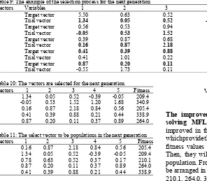
Table 9: The example of the selection process for the next generation
Vectors Variables 1 2 3 4 5 Fitness
1 Target vector 5.50 0.63 0.52 0.37 0.17 210.1
Trial vector 1.34 0.05 0.52 -0.39 -0.05 209.4
2 Target vector 0.56 0.53 0.94 0.55 0.73 343.9
Trial vector -0.05 0.53 1.52 1.20 1.68 340.9
3 Target vector 0.39 0.87 0.68 0.84 0.56 345.0
Trial vector 0.16 0.87 2.18 0.84 0.56 205.4
4 Target vector 0.41 0.39 0.88 0.21 0.44 338.9
Trial vector 0.41 1.01 0.22 0.87 0.44 344.3
5 Target vector 0.87 0.20 0.11 0.37 0.89 264.0
Trial vector -0.55 1.73 0.11 1.15 0.89 344.3
Table 10: The vectors are selected for the next generation
Vectors 1 2 3 4 5 Fitness
1 1.34 0.05 0.52 -0.39 -0.05 209.4
2 -0.05 0.53 1.52 1.20 1.68 340.9
3 0.16 0.87 2.18 0.84 0.56 205.4
4 0.41 0.39 0.88 0.21 0.44 338.9
5 0.87 0.20 0.11 0.37 0.89 264.0
Table 11: The select vector to be populations in the next generation
Vectors 1 2 3 4 5 Fitness
1 0.16 0.87 2.18 0.84 0.56 205.4
2 1.34 0.05 0.52 -0.39 -0.05 209.4
3 0.78 0.63 0.52 0.37 0.17 210.1
4 0.87 0.20 0.11 0.37 0.89 264.0
5 0.41 0.39 0.88 0.21 0.44 338.9
Selection, the next Generation is selected (G+1): the better solutions are selected by comparison the fitness value from the target vector and the trial vector for cases in which the fitness value of the trial vector is lower than the target vector. Therefore, the trial vector is selected as the next generation as in Eq. 20. The example of the selection process and the vectors are selected for the next generation as present in Table 9 and Table 10, respectively:
(20)
i, j, G
i, j, G i, j, G i, j, G
i, j, G
X
U if f U f
X otherwise
X
Where:
Ui, j, G = Target vector in the next generation
Xi, j, G+1= Target vector in the next generation
Calculation using the DE/rand/2/bin: DE/rand/2/bin and DE/rand/2/exp have step similar to DE/rand/1/bin and DE/rand/1/exp but have different calculations in mutation step as Eq. 21:
(21)
r1,i, G r2,i,G i, j, G r5,i, G
r3,i, G r4,i,G
X +X
-V X +F×
X -X
The improved differential evolution algorithm for solving MFLP: In this research, the answer was improved in the selection process by selecting vectors whichprovidethe better solutions with comparing the fitness values from both trial vector and target vector. Then, they will be chosen to be the next generation of population. From Table 10, the order of fitness values can be arranged in ascending order as follows: 205.4, 209.4, 210.1, 264.0, 338.9, 340.9, 343.9, 344.3, 344.3 and 345.0 which will be selected as the population in the next 5 first vectors as shown in Table 11.
The compared results of the improved DE algorithm, DE algorithm and the other methods: In the experiment, solving MFLP applies a VBA program running on a laptop, Core i5, 2.5 GHz, 12 GB RAM, Windows 10 operating system. It calculates and shows the result and the layout on spreadsheet.
Due to multi-floor facility layout problems, there are a variety of limitations and the scope is different. Researchers studying this problem, creates different definitions of the problem. Therefore, there is still no standard answer to this problem. Therefore, in this research, compared with the multiple and SABLE methods by Meller (1992) which have similar problems. Multiple and SABLE considered only the cost of material handling. Therefore, in the determination value of W1 is
1 and W2 is 0 Table 12.
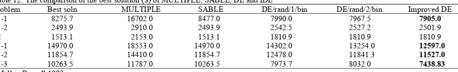
Table 12: The comparison of the best solution ($) of MULTIPLE, SABLE, DE and IDE
Problem Best soln MULTIPLE SABLE DE/rand/1/bin DE/rand/2/bin Improved DE
11-1 8275.7 16702.0 8477.0 7990.0 7967.5 7905.0
11-2 2493.9 2910.0 2493.9 2542.5 2527.2 2501.9
12 1513.1 2153.0 1513.1 1810.9 1810.9 1810.9
21-1 14970.0 18553.0 14970.0 14302.0 13254.0 12597.0
21-2 11854.7 14410.0 11854.7 12478.0 11841.3 11527.0
21-3 10263.5 11787.0 10263.5 7973.7 8032.0 7438.83
[image:8.612.71.544.237.428.2]*Meller, Russell 1992
Table 13: The average of the material transportation cost ($) for MULTIPLE, SABLE, DE and IDE
MULTIPLE SABLE DE/rand1/bin DE/rand/2/bin Improved DE
---Problem x x x x x
11-1 16702.02 8958.67 8124.29 8097.50 8056.00
11-2 2910.67 2558.09 2611.48 2689.70 2585.80
12 2153.09 1640.34 1935.78 1943.44 1889.83
21-1 18553.50 16310.40 15750.10 16150.35 15199.60
21-2 14410.57 12745.74 13699.80 13069.90 12614.50
21-3 11787.28 10788.89 8856.43 8839.25 8268.55
Table 14: A worst analysis based on minimum cost solutions
Best soln MULTIPLE SABAL DE/rand/1/bin DE/rand/2/bin Improved DE
---Problem Min Max Max Max Max Max
11-1 8275.70 21982.17 14956.30 8370.00 8309.00 8325.00
11-2 2493.92 3332.41 2662.70 2777.01 2770.93 2742.51
12 1513.15 2538.05 1842.50 2120.45 2080.85 2070.15
21-1 14970.00 21408.00 17774.40 18201.00 19902.00 16852.00
21-2 11854.70 17262.33 14230.70 14618.70 13979.00 13481.30
21-3 10263.50 13072.00 11273.70 9714.66 9566.50 9340.83
the MFLP by using the basic DE algorithm consisted of two methods as follows: DE/rand/1/bin and DE/rand/2/bin, the IDE on DE/rand/1/bin.
The comparison of the best solution: The cost of material transportation of comparison with the best solution from Meller, Russell (Meller and Bozer, 1997) are in the Table 12.
From the experimental results in Table 13, the IDE can generate the optimal solutions better than MULTIPEL is 52.67, 14.02, 15.89, 32.10, 20.01 and 36.92% for problems 11-1, 11-2, 12, 21-1, 21-2 and 21-3, respectively and can generate the optimal solution that is better than the SABLE is 6.75, 15.85, 2.76 and 27.56% for problems 11-1, 21-1, 21-2 and 21-3, respectively.
The comparison of the average: The average on the experiment 10 times on problem 11-1, 11-2, 12, 21-1, 21-2 and 21-3 are in Table 13.
From the experimental results in Table14, the average of the best solutions generated from the IDE method are lower than the average of the best solutions generated from the DE/rand/1/bin and DE/rand/2/bin in all problems. Especially in theproblems11-1, 21-1, 21-2 and 21-3, the mean of the best solution generated from the IDE method is lower than the average of the best answer from both the multiple and SABLE by comparing the average of the best solution from the IDE and SABLE. It is found that the IDE method has the best mean values that are lower or better than 10.08, 6.81, 1.03 and 23.36%, respectively.
From the results of the comparison of the worst values in Table 16, it was found that the worst values obtained from the three different methods of evolution were lower than the worst values obtained from the multiple. The IDE method is lower than the worst value obtained from the SABLE method in all three large problems 21-1, 21-2 and 21-3 and the worst value obtained from the IDE method is lower than a worst value from the basic DE in problem 12, 21-1, 21-2 and 21-3.
CONCLUSION
This study has presented the improved differential evolution algorithm for multi-floor facility layout problems. The objectives are minimize the transportation material and maximize the adjacency between facilities. A comparison with the other methods such as MULTIPLE, SABLE and basic DE were performed to evaluate the proposed algorithm’s efficiency. The comparison show that the proposed algorithm is superior to the existing one.
In the future work, aiming at solving large-scale problems with more complex and more difficult such as multi-floor facility layout problems with elevator utilization and waiting time or dynamic facility layout problems.
ACKNOWLEDGEMENTS
We would like to thank Industrial Engineering Department, Faculty of Engineering, Ubon Ratchathani University and my family, teachers, staffs and friends for their support and encouragement.
REFERENCES
Abdinnour-Helm, S. and S.W. Hadley, 2000. Tabu search based heuristics for multi-floor facility layout. Int. J. Prod. Res., 38: 365-383.
Afrazeh, A., A. Keivani and L.N. Farahani, 2010. A new model for dynamic multi floor facility layout problem. Adv. Model. Optim., 12: 249-256.
Armour, G.C. and E.S. Buffa, 1963. A heuristic algorithm and simulation approach to relative location of facilities. Manage. Sci., 9: 294-309.
El-Ela, A.A.A., M.A. Abido and S.R. Spea, 2010. Optimal power flow using differential evolution algorithm. Electric Power Syst. Res., 80: 878-885. Huang, C., C.K. Wong and C.M. Tam, 2010.
Optimization of material hoisting operations and storage locations in multi-storey building construction by mixed-integer programming. Automation Construc., 19: 656-663.
Johnson, R.V., 1982. Spacecraft for multi-floor layout planning. Manage. Sci., 28: 407-417.
Kochhar, J.S. and S.S. Heragu, 1999. Facility layout design in a changing environment. Int. J. Prod. Res., 37: 2429-2446.
Kochhar, J.S., 1998. MULTI-HOPE: A tool for multiple floor layout problems. Intl. J. Prod. Res., 36: 3421-3435.
Krishnan, K.K., A.A. Jaafari, M. Abolhasanpour and H. Hojabri, 2009. A mixed integer programming formulation for multi-floor layout. Afr. J. Bus. Manage., 3: 616-620.
Kuila, P. and P.K. Jana, 2014. A novel differential evolution based clustering algorithm for wireless sensor networks. Appl. Soft Comput., 25: 414-425.
Lee, K.Y., M.I. Roh and H.S. Jeong, 2005. An improved genetic algorithm for multi-floor facility layout problems having inner structure walls and passages. Comput. Oper. Res., 32: 879-899.
Matsuzaki, K., T. Irohara and K. Yoshimoto, 1999. Heuristic algorithm to solve the multi-floor layout problem with the consideration of elevator utilization. Comput. Ind. Eng., 36: 487-502.
Meller, R.D. and Y.A. Bozer, 1996. A new simulated annealing algorithm for the facility layout problem. Int. J. Prod. Res., 34: 1675-1692.
Meller, R.D. and Y.A. Bozer, 1997. Alternative approaches to solve the multi-floor facility layout problem. J. Manuf. Syst., 16: 192-203.
Meller, R.D., 1992. Layout algorithms for single and multiple floor facilities. Ph.D Thesis, University of Michigan, Ann Arbor, Michigan.
Seehof, J.M. and W.O. Evans, 1967. Automated layout design program. J. Ind. Eng., 18: 690-695.
Shahnazari-Shahrezaei, P., R. Tavakkoli-Moghaddam, M. Azarkish and A. Sadeghnejad-Barkousaraie, 2012. A differential evolution algorithm developed for a nurse scheduling problem. South Afr. J. Ind. Eng., 23: 68-90.
Singh, S.P. and R.R.K. Sharma, 2006. A review of different approaches to the facility layout problems. Int. J. Adv. Manuf. Technol., 30: 425-433.
Sresracoo, P., N. Kriengkorakot, P. Kriengkorakot and K. Chantarasamai, 2018. U-shaped assembly line balancing by using differential evolution algorithm. Math. Comput. Appl., Vol. 23,
Tompkins, J., J. White and Y. Bozer, 2010. Facilities Planning. 4th Edn., John Wiley and Sons, United State of America, ISBN: 9780470444047, Pages: 845.
Xiaoning, Z. and Y. Weina, 2011. Research on layout problem of multi-layer logistics facility based on simulated annealing algorithm. Proceedings of the 2011 4th International Conference on Intelligent Computation Technology and Automation, March 28-29, 2011, IEEE, Shenzhen, China, pp: 892-894. Xu, H. and J. Wen, 2012. Differential evolution algorithm
for the optimization of the vehicle routing problem in logistics. Proceedings of the 2012 Eighth International Conference on Computational Intelligence and Security, November 17-18, 2012, IEEE, Guangzhou, China, pp: 48-51.