warwick.ac.uk/lib-publications
Manuscript version: Author’s Accepted Manuscript
The version presented in WRAP is the author’s accepted manuscript and may differ from the published version or Version of Record.
Persistent WRAP URL:
http://wrap.warwick.ac.uk/125497
How to cite:
Please refer to published version for the most recent bibliographic citation information. If a published version is known of, the repository item page linked to above, will contain details on accessing it.
Copyright and reuse:
The Warwick Research Archive Portal (WRAP) makes this work by researchers of the University of Warwick available open access under the following conditions.
Copyright © and all moral rights to the version of the paper presented here belong to the individual author(s) and/or other copyright owners. To the extent reasonable and
practicable the material made available in WRAP has been checked for eligibility before being made available.
Copies of full items can be used for personal research or study, educational, or not-for-profit purposes without prior permission or charge. Provided that the authors, title and full
bibliographic details are credited, a hyperlink and/or URL is given for the original metadata page and the content is not changed in any way.
Publisher’s statement:
Please refer to the repository item page, publisher’s statement section, for further information.
Distinguishing newforms
∗Sam Chow† University of Bristol [email protected]
Alexandru Ghitza‡ University of Melbourne [email protected]
September 9, 2019
Abstract
Letn0(N, k) be the number of initial Fourier coefficients necessary to distinguish newforms of level N and even weight k. We produce extensive data to support our conjecture that ifN is a fixed squarefree positive integer andkis large thenn0(N, k) is the least prime that does not divide N.
1
Introduction
The predominant way of specifying a modular form is via its Fourier expansion
f(q) =
∞
X
n=0
an(f)qn. (1.1)
Since this power series representation involves infinitely many coefficients, a natural ques-tion is whether one can recognise a given formf by looking at only finitely many (initial) coefficients. This is the object of a classical result of Sturm:1
Theorem 1.1([23], see also [18]). Let N, k∈Z>0, and let f, g∈Mk(Γ0(N))withf 6=g.
Then there exists
n≤ k
12[SL2(Z) : Γ0(N)] (1.2) such thatan(f)6=an(g).
We refer to (1.2) as the Sturm bound. It is sharp at this level of generality. However, many modular forms that occur naturally in applications (especially in number-theoretic contexts) have additional properties, such as being eigenvectors for the Hecke operators. We ask the question: Is it possible to sharpen the Sturm bound in the presence of this extra information? More precisely, let n0 =n0(N, k) be the smallest nonnegative integer such
that the following statement is true:
∗
Thanks to James Withers for running some of the code. We also thank David Loeffler, M. Ram Murty, Abhishek Saha and Fredrik Str¨omberg for useful comments.
†
The first author was supported by the Elizabeth and Vernon Puzey scholarship, and is grateful towards the University of Melbourne for their hospitality while preparing this memoir.
‡
The second author was supported by Discovery Grant DP120101942 from the Australian Research Council.
1Theorem 1.1 is a special case of Sturm’s main result, which is concerned with congruences between
Let f, g ∈ Sk(Γ0(N)) be newforms such that an(f) = an(g) for all n ≤ n0.
Then f =g.
The main problem studied in this paper is the dependence of n0 on the parametersN
andk, forN, k∈Z>0. Note that if kis odd then n0 = 0, sinceSk(Γ0(N)) ={0}(see [12,
p. 15]). We therefore restrict attention to even weights k. The empirical data that we computed strongly support the following stability conjecture for squarefree levels:
Conjecture 4.1. Let N ∈ Z>0 be squarefree. Then there exists K ∈ Z>0 such that if
k≥K is an even integer then n0(N, k) is equal to the least prime that does not divideN.
We note that the least prime that does not divideN is bounded above by 2(logN+ 1); see the proof of [6, Theorem 1]. The data also indicate a stability phenomenon in the non-squarefree level case, but we have not found a simple conjectural characterisation of the eventual value ofn0 in this situation—there are cases where it appears to exceed the
least prime that does not divideN. We can prove the “easy half” of Conjecture 4.1:
Theorem 4.4. Let N ∈Z>0, and let k≥38 be an even integer. Then n0(N, k) is greater
than or equal to the least prime that does not divideN.
One might reasonably ask how largeKneeds to be in Conjecture 4.1. The data suggest K= 38 as a candidate for 1≤N ≤30 andK= 8 for 30< N ≤100 (squarefreeN). Does K= 38 suffice uniformly, or mightK need to depend onN? The answer is not clear from the results of our computations, however it does seem that we can always takeK to be quite small.
Many authors have studied the recognition problem for modular forms, e.g. [2], [3], [6], [8], [10], [13], [14], [17], [18], [23]. Maeda’s conjecture (Conjecture 5.1) would imply thatn0(1, k)≤2 for all k∈Z>0, and from this and [15, Theorem 1] it would follow that
n0(1, k) = 2 for all even numbers k ≥ 28. The second author and J. Withers [9] have
proposed a generalisation of Maeda’s conjecture that would imply Conjecture 4.1; this is discussed in§5.
Our algorithm for evaluating n0(N, k) is based on the fact that if f is a normalised
Hecke eigenform and n∈ Z>0 then an(f) equals the eigenvalue of f with respect to the Hecke operator Tn. Moreover, it suffices to consider Tp for primes p (see Lemma 3.1). We consider intersections of Tp-eigenspaces over all primes p up to a point (call such intersections “homes”). Any home H has a basis given by its newforms, so the number of newforms inH is equal to dimH. We continue until there are no homes of dimension greater than one.
Two main refinements improve the efficiency of our algorithm. We use modular symbols instead of modular forms (see (2.5)). Our second improvement is harder to describe. The idea is to factorise overQthe characteristic polynomial ofTp, considering the kernel of each irreducible factor. We intersect these kernels for small primes p, and run our algorithm on each such intersection. This enables us to work in smaller spaces, reducing the need to manipulate large matrices.
This paper is organised as follows. In §2, we clarify definitions and recall key results. In §3, we describe in detail our algorithm for computing n0(N, k). In §4, we discuss
Conjecture 4.1 in more detail. In particular, we prove Theorem 4.4, and further address the case whereN is not squarefree. Finally, in§5, we relate Conjecture 4.1 to a conjecture of the second author and J. Withers.
For k ∈Z>0 and Γ a congruence subgroup, we denote byMk(Γ) the complex vector
symbol p is reserved for primes. For r ∈ Z>0, we write pr for the rth smallest prime
number. We shall writeω(N) for the number of distinct prime divisors ofN. The algebraic closure ofQwill be denotedQ.
2
Some background
In this section we recall some standard definitions and results. LetN, k∈Z>0. We shall work in
S:=Sknew(Γ0(N)), (2.1)
the new subspace of Sk(Γ0(N)). Here we refer the reader to [4, §I.6]. (The spaceS was
first defined in [1].)
For each n∈Z>0 we have a Hecke operatorTn acting onS, and these commute (see
[5, §5.3] and [20, Ch. 9]). The Hecke algebra is the commutative ring generated by the Tn:
T=Z[T1, T2, . . .].
A Hecke eigenform is a modular form that is an eigenvector of Tn for every n. A Hecke eigenform isnormalised ifa1(f) = 1, wherea1(f) is as in (1.1). By [20, Proposition 9.10],
iff is a normalised Hecke eigenform then
Tnf =an(f)f (n∈Z>0), (2.2)
wherean(f) is as in (1.1). This means that we can compare Fourier coefficients by study-ing eigenvalues and eigenspaces of the operators Tn. A newform (in Sk(Γ0(N))) is a
normalised Hecke eigenform that lies inS. The proof of [5, Theorem 5.8.2] shows that the set of newforms inS is a basis for S. In particular, the spaceS contains precisely dimS newforms.
Letn∈Z>0. From [16, Theorem 4.5.19] (see also [19, Theorem 3.48]), we see that the
characteristic polynomial χn of Tn acting on Sk(Γ0(N)) has rational integer coefficients.
Iff ∈Sk(Γ0(N)) is a normalised Hecke eigenform then it follows from (2.2) thatan(f) is a root ofχn, and is therefore an algebraic integer.
To hasten our calculations, we use modular symbols. There is aT-module isomorphism
Φ :S →Snewk (Γ0(N);C)+ (2.3)
between S and the plus subspace of the new subspace of the vector space of cuspidal weightkmodular symbols for Γ0(N) overC(see [20, Theorem 8.23] and the discussion on [20, p. 165]). We perform many of our calculations inS∗ :=Snewk (Γ0(N);Q)+. The Hecke algebra acts onS∗, and there are isomorphisms
S∗⊗F 'Snewk (Γ0(N);F)+ (F =Q,C) (2.4)
ofT-modules. These isomorphisms follow from the definitions in [20, Ch. 8].
LetB =B(N, k) be the Sturm bound, and letf1, . . . , fdbe the newforms in S. There existr1, . . . , rB∈Q such that
X
n≤B
rnan(fi)6= X n≤B
rnan(fj) (1≤i < j≤d).
plus P times the second column plus P2 times the third column, and so on.) The linear operatorT =P
n≤BrnTn acts irreducibly onS, since its eigenvalues are distinct. Hence, by (2.3) and (2.4), the linear operatorT acts irreducibly onS∗⊗C, and therefore uniquely defines a basis of eigenvectors, up to rescaling. The spaceS∗⊗Qis stable under this action, and Q is algebraically closed, so S∗⊗Q must have a basis B of eigenvectors for T. By (2.3) and (2.4), the modular symbols Φ(f1), . . . ,Φ(fd) form a basis of eigenvectors for the action of T on S∗⊗C. For i= 1,2, . . . , d, choosesi ∈ B equal to a constant times Φ(fi). Nowfi7→si (1≤i≤d) is a T-module isomorphism
Sknew(Γ0(N);Q)'S∗⊗Q. (2.5)
3
The algorithm for computing
n
0(
N, k
)
LetN, k∈Z>0, and recall (2.1). We begin with the following observation:
Lemma 3.1. Let f, g ∈ Mk(Γ0(N)) be normalised Hecke eigenforms. Suppose an(f) 6=
an(g) for some n∈Z>0. Then there exists a prime divisor pof nsuch thatap(f)6=ap(g).
Proof. This follows from (2.2) and [5, (5.10)], upon noting that Tmn = TmTn whenever (m, n) = 1 (see [5, §5.3]).
In view of (2.2), we now see that if dimS ≥2 thenn0(N, k) is the least prime` such
that there do not exist distinct newforms f, g ∈ S such that f and g have the same Tp eigenvalues for each primep≤`. Our basic algorithm is as follows:
Algorithm 3.2. Build S.
1. If dimS <2, return 0.
2. Consider the eigenspaces of the action of T2 onS. LetA1, . . . , Aa be the eigenspaces
of dimension greater than one, and call these the homes forT2. If a= 0, return 2.
3. Consider the eigenspaces of the action ofT3onS, and intersect these withA1, . . . , Aa,
separately. Let B1, . . . , Bb be the intersections of dimension greater than one, and call these the homes for T3. If b= 0, return 3.
4. Repeat for T5, T7, T11, . . ..
As the newforms in S are linearly independent, the dimension of any subspace of S is greater than or equal to the number of newforms it contains. Thus, by the above discussion, the Sturm bound implies that Algorithm 3.2 terminates and returns an upper bound forn0. In fact the output of Algorithm 3.2 is exactly n0, since we can show that
the dimension of any “home” is equal to the number of newforms it contains:
Lemma 3.3. Every home, as defined in steps 2 and 3 of Algorithm 3.2, has a basis given by its newforms.
Proof. We induct on primes. As discussed in §2, the space S has a basis given by its newforms. Letpbe prime. Ifp= 2, letH=S. Otherwise, letH be a home for the Hecke operator corresponding to the prime before p. Our inductive hypothesis is that the set {f1, . . . , fd}of newforms in H is a basis for H. LetB be a home for Tp that comes from intersecting withH in step 3 of Algorithm 3.2 (if p = 2, let B be any home for T2). It
Note thatTp acts on H, since the Hecke operators commute. Further, the homeB is an eigenspace of this action. Recalling (1.1), and letting ap(fi) =λi (1≤i≤d), we see that the characteristic polynomial of this action isQ
i≤d(X−λi). Letλbe the eigenvalue associated to B, and let I be the set of i ∈ {1,2, . . . , d} such that λi = λ. The set of newforms in B is {fi :i∈I}. This is a basis for B, being a linearly independent subset of size|I|= dimB.
Using the software Sage [21], we may implement Algorithm 3.2. It suffices to work over Q, since the Fourier coefficients of normalised Hecke eigenforms are algebraic. Moreover, by (2.5), we may use modular symbols instead of modular forms. These changes improve the speed of our algorithm. They are implemented in Sage as follows:
Algorithm 3.4. Build S∗ =Snewk (Γ0(N);Q)+. Suppose we wish to build the eigenspaces for the action of a Hecke operator on Sknew(Γ0(N);Q). Compute the matrix of its action onS∗, then use the command
base_extend
to consider it as a matrix with entries in Q. Build the eigenspaces for this matrix.
We thus produce the eigenspaces inS∗⊗Q, which correspond via (2.5) to the eigenspaces in Sknew(Γ0(N);Q). The drawback of the algorithm as described thus far (that is, mod-ifying Algorithm 3.2 using Algorithm 3.4) is that it requires the manipulation of large matrices. To overcome this, we introduce the following refinement:
• Let q be a prime number.
• Consider, as a polynomial in T2, the characteristic polynomial of the action of T2
on S∗. Factorising this overQ, consider the irreducible factors of dimension greater than 1, and take their kernels. Call these the streets forT2.
• Compute the corresponding kernels with T3 in place ofT2, intersect them with the
streets for T2, and take the intersections of dimension greater than one. Call these
the streets forT3.
• Repeat for T5, . . . , Tq.
• Return the streets forTq, and call these the final streets.
Let q be prime, let F be a final street, and let F0 = F ⊗Q. We seek to show that running the algorithm withF in place of S∗ returns the smallest integer m such that if f, g∈ F0 are newforms such that a
n(f) =an(g) for alln≤m thenf =g (newforms are understood with reference to (2.5)). For this purpose, it suffices to obtain the appropriate analogue to Lemma 3.3. By the proof of Lemma 3.3, it remains to show that F0 has a basis given by its newforms.
Lemma 3.5. Let q be prime, and letF be a corresponding final street. Then F ⊗Q has a basis given by its newforms.
of newforms inF is a basis forF. Consider the characteristic polynomialχp of the action ofTp onS. Factorising χp overQ, letP1, . . . , Ptbe the distinct monic irreducible factors,
and let Xj = F ∩kerPj(Tp) (1 ≤ j ≤ t). It remains to show that each Xj has a basis given by its newforms.
Recall (1.1), and letap(fi) =λi (1≤i≤d). Fixj∈ {1,2, . . . , t}, and let I be the set of i∈ {1,2, . . . , d} such that Pj(λi) = 0. The set of newforms in Xj is {fi :i∈I}. This set is linearly independent, so it remains to show that it spansXj. Letf ∈Xj, and write f =c1f1+. . .+cdfd withc1, . . . , cd∈Q. Now
0 =Pj(Tp)(c1f1+. . .+cdfd) = X
i≤d
ciPj(λi)fi,
so ci = 0 whenever i /∈ I. Now f lies in the span of {fi : i ∈ I}, which completes the proof.
Letq be a prime number, and build the final streets as above. We run our algorithm on each of the final streets, and consider the maximum output,m. Supposem≥q. There exist distinct newforms f, g ∈ S whose Fourier coefficients satisfy ap(f) = ap(g) for all primesp < m; son0≥m. Further, there cannot exist distinct newformsf, g∈S such that
ap(f) =ap(g) for all primes p≤m (otherwise they would be in F ⊗Q for the same final streetF, contradicting the fact thatmwas the maximum output obtained by running the algorithm on the final streets). Hencen0≤m, so we must haven0 =m.
To summarise the above discussion, if the maximum output is greater than or equal to our chosen prime number q, then it equals n0. Thus, the following procedure returns
n0(N, k):
• If dimS <2, return 0.
• Chooseq= 7, and run the algorithm on each of the final streets, taking the maximum output m. If m≥q, returnm.
• Repeat for q= 5,3,2.
• Return 2.
For efficiency, we adopt one final finesse. By similar reasoning to above, we note that if m < q then n0 ≤ q. We can sometimes use this to deduce the value of n0 without
completing every step of the algorithm. For instance, if we know thatn0 ≤ 7, and that
one of the final streets forq = 5 returns 7, then we must have n0 = 7. Our full Sage [21]
code may be found at the second author’s webpage.2 A sample of the resulting data is given in the appendix.
4
The stability conjecture
Our data suggest that ifN is fixed thenn0(N, k) stabilises askincreases (keven); see the
appendix. The evidence is particularly compelling whenN is squarefree, and we propound a more precise statement in this case:
Conjecture 4.1. Let N ∈ Z>0 be squarefree. Then there exists K ∈ Z>0 such that if k≥K is an even integer then n0(N, k) is equal to the least prime that does not divideN.
Part of this conjecture can be obtained from the following result:
Theorem 4.2 (Atkin-Lehner [1, Theorem 3]). Let N, k ∈ Z>0, let f ∈ Sk(Γ0(N)) be a
newform, and letp be a prime dividing N.
(a) If p2 |N thenap(f) = 0.
(b) If p2 -N thenap(f) =±p k
2−1.
So for primes p | N, the eigenvalue ap(f) is heavily prescribed, which makes the operatorTp particularly bad at telling apart eigenforms. Thus, we would expectn0(N, k)
to be greater than or equal to the least prime that does not divideN. This is indeed the case if the spaceS =Sknew(Γ0(N)) is sufficiently large:
Corollary 4.3. LetN, k∈Z>0. Lett∈Z≥0 be the number of consecutive primes, starting
from2, that divide N (so pt+1 is the least prime that does not divide N). Suppose
dimS >2t.
Thenn0 is greater than or equal to the least prime that does not divide N.
Proof. Let i ∈ {1,2, . . . , t}, and note that pi | N. By Theorem 4.2, there are at most 2 possible values for the pi-th coefficient of a newform in S. (There is one possibility if p2i |N, and two possibilities if p2i -N.)
SinceS has a basis given by its newforms, there exist dimS ≥2t+ 1 distinct newforms in S. By the pigeonhole principle, there exist at least 2t−1+ 1 distinct newforms in S with the same Fourier coefficient a2. Among these, there exist at least 2t−2+ 1 distinct
newforms with the same a3. Continuing in this way, there exist at least 2t−t+ 1 = 2
distinct newforms with the same a2, a3, a5, . . . , apt. We conclude that n0 ≥pt+1.
Martin [15, Theorem 1] provides a formula for dimS. Combining it with Corollary 4.3 gives rise to the “easy half” of Conjecture 4.1:
Theorem 4.4. Let N ∈Z>0, and let k≥38 be an even integer. Then n0(N, k) is greater
than or equal to the least prime that does not divideN.
Proof. Ask >2 is even, Martin [15, Theorem 1] gives
dimS = (k−1)N s+0(N)/12−v∞+(N)/2 +c2(k)v2+(N) +c3(k)v3+(N), (4.1)
wheres+0,v∞+,c2,v+2,c3 andv3+ are certain quickly computable arithmetic functions.
First suppose N ≥1000. We deduce from (4.1) and the definitions of the arithmetic functions therein that
dimS≥(k−1)N/12×Y p|N
(1−p−1−p−2)−√N /2−17/12×2ω(N).
Sincet≤ω(N) in Corollary 4.3, it now remains to show that
k >1 + 12/N ×( √
N /2 + 29/12×2ω(N))×Y p|N
(1−p−1−p−2)−1. (4.2)
We may easily verify the bounds
Y
p|N
(9/5)ω(N) <2.8N1/4 and 2ω(N)<5N1/4. Since
k≥38>1 + 6.23(6N−1/4+ 145N−1/2) for allN ≥1000, we now have (4.2).
For N = 2,4,6,12, we shall use (4.1) to check that the hypothesis of Corollary 4.3 is met. We note that −3/4 < c2(k) ≤ 1/4 and −2/3 < c3(k) ≤1/3. If N = 2 then (4.1)
yields
dimS= (k−1)/12−c2(k)−2c3(k)≥37/12−1/4−2/3>2 = 2t.
IfN = 4 then (4.1) yields
dimS = (k−1)/12−c2(k) +c3(k)>37/12−1/4−2/3>2 = 2t.
IfN = 12 then (4.1) yields
dimS = (k−1)/6 + 2c2(k)−c3(k)>37/6−3/2−1/3>4 = 2t.
ConsiderN = 6. By (4.1), it suffices to prove that
(k−1)/6 + 2c2(k) + 2c3(k)>4.
We can verify this directly fork= 38,40, while ifk≥42 then
(k−1)/6 + 2c2(k) + 2c3(k)>41/6−3/2−4/3 = 4.
Finally, suppose that N < 1000 with N /∈ {2,4,6,12}. By direct computation, we have
k≥38>1 +12(v
+
∞(N)/2 + 3|v2+(N)|/4 + 2|v+3(N)|/3 + 2t)
N s+0(N) .
The proof is completed via (4.1) and Corollary 4.3, recalling that |c2(k)| < 3/4 and
|c3(k)|<2/3.
The following example suggests that the non-squarefree level case is more complicated. We take the following definition from [24, p. 2]. LetN, k ∈Z>0, let f ∈Sk(Γ0(N)), and
letχ be a Dirichlet character. The twist off by χ is given by
f ⊗χ(q) =
∞
X
n=1
χ(n)an(f)qn.
Example 4.5. Let S =Sknew(Γ0(49)), and let χ be the Legendre symbol modulo 7, i.e.
χ(n) = n
7
(n∈Z).
For each k ∈ {4,6,8,10,12}, we observe newforms f, g ∈ S such that f = g⊗χ and g=f⊗χ. As χ(2) = 1, we have a2(f) =a2(g), so T2 fails to distinguish f andg.
This phenomenon is closely related to the existence of CM forms (see [24, p. 2]). Indeed, in the example abovef+g has complex multiplication byχ. It is likely that the formsf and g, although “new” in the usual sense (not arising from Γ0(7) or Γ0(1)), are
coming from a different congruence subgroup Γ of level 7. For an explanation of this type of behaviour for Γ0(9), see [22].
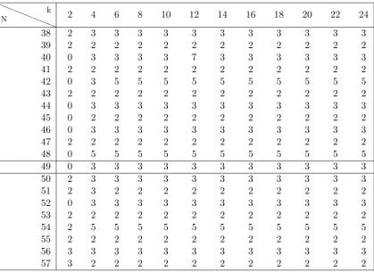
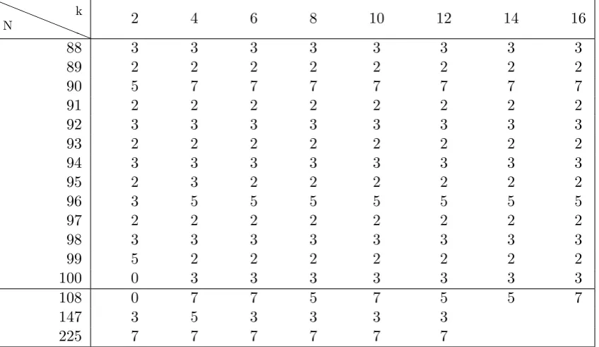
There may be a more general stability phenomenon which also encompasses non-squarefree values of N. In the cases N = 49,108,147,225, one might predict from the data thatn0 stabilises towards a prime that exceeds the least prime that does not divide
N (see Tables 5 and 8). For all other values of N that we examined, it would appear thatn0 stabilises towards the least prime that does not divide N. Does there always exist
5
Irreducibility of Hecke polynomials
A Hecke polynomial is the characteristic polynomial of a Hecke operator Tn acting on a space of modular forms. In the 1970s, Maeda observed that the Hecke polynomials of T2
on Sk(SL2(Z)) are irreducible overQ for all k such that dimSk(SL2(Z))≤12. Over the next 20 years, this observation matured into the following statement:
Conjecture 5.1 (Maeda [11]). Let k ∈ Z>0, n ∈ Z>1, and let F ∈ Z[X] be the char-acteristic polynomial of the Hecke operator Tn acting on S := Sk(SL2(Z)). Then F is
irreducible overQ and its Galois group Gis isomorphic to the symmetric group ΣdimS.
We refer the reader to [7] for a survey of results on Maeda’s conjecture and a report on its verification for the operatorT2 and weightsk≤14 000.
In [24], Tsaknias considers higher-level generalisations of the following weak version of Conjecture 5.1: there is a unique Galois orbit of Hecke eigenforms in Sk(SL2(Z)). We describe his findings in the squarefree level case. If N = p1p2. . . pt is squarefree, the Atkin-Lehner involutionswpi decompose the space of newforms into eigenspaces
Sknew(Γ0(N)) =
M
∈{±1}t S.
Tsaknias’s computations indicate that, fork large enough, the spaceSknew(Γ0(N)) has 2t
Galois orbits of newforms. The second author and J. Withers [9] have investigated higher-level analogues of the full Maeda conjecture. Their experiments suggest the following statement in the squarefree level case:
Conjecture 5.2. Let N ∈ Z>0 be squarefree. Then there exists K0 ∈Z>0 such that the following hold wheneverk≥K0 is even and n≥2 is coprime to N:
(a) The characteristic polynomial F of the Hecke operator Tn acting on Sknew(Γ0(N)) is
separable (that is, F has no repeated roots over Q).
(b) The Atkin-Lehner decomposition
Sknew(Γ0(N)) =
M
S
is the only obstacle to the irreducibility of the polynomialF.
These statements have been verified computationally for squarefree N ≤ 200, even weightsk ≤30 and operatorsTp forp < 100 prime and not dividing N. Our immediate interest in Conjecture 5.2 is the following result:
Theorem 5.3. Part (a) of the generalised Maeda Conjecture 5.2 implies the stability Conjecture 4.1.
Proof. Let N ∈ Z>0 be squarefree. Let K = max{38, K0}, with K0 provided by
Conjec-ture 5.2. Let p be the least prime that does not divide N, and let k ≥ K be even. By Theorem 4.4, we have n0(N, k) ≥ p. So it suffices to show that if f, g ∈ Sk(Γ0(N)) are
distinct newforms thenap(f)6=ap(g).
Let B={f1, f2, . . . , fd} be the newforms in Sk(Γ0(N)), where d= dimSknew(Γ0(N)).
Appendix: Data
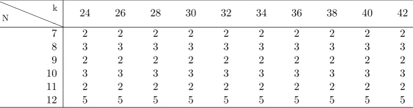
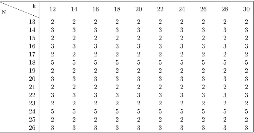
We tabulaten0 =n0(N, k) forkeven (ifk is odd thenn0 = 0). We putN on the vertical
[image:11.595.88.510.196.305.2]axis andk on the horizontal axis, so that along any rowN is fixed andkvaries. A larger set of data may be found at the second author’s webpage.3
Table 1: Some values ofn0(N, k).
a a
a a
a a
a
N
k
38 40 42 44 46 48 50 52 54 56
1 2 2 2 2 2 2 2 2 2 2
2 3 3 3 3 3 3 3 3 3 3
3 2 2 2 2 2 2 2 2 2 2
4 3 3 3 3 3 3 3 3 3 3
5 2 2 2 2 2 2 2 2 2 2
6 5 5 5 5 5 5 5 5 5 5
Table 2: More values of n0(N, k).
a a
a a
a a
a
N
k
24 26 28 30 32 34 36 38 40 42
7 2 2 2 2 2 2 2 2 2 2
8 3 3 3 3 3 3 3 3 3 3
9 2 2 2 2 2 2 2 2 2 2
10 3 3 3 3 3 3 3 3 3 3
11 2 2 2 2 2 2 2 2 2 2
12 5 5 5 5 5 5 5 5 5 5
3
[image:11.595.89.509.375.485.2]Table 3: More values of n0(N, k).
a a
a a
a a
a
N
k
12 14 16 18 20 22 24 26 28 30
13 2 2 2 2 2 2 2 2 2 2
14 3 3 3 3 3 3 3 3 3 3
15 2 2 2 2 2 2 2 2 2 2
16 3 3 3 3 3 3 3 3 3 3
17 2 2 2 2 2 2 2 2 2 2
18 5 5 5 5 5 5 5 5 5 5
19 2 2 2 2 2 2 2 2 2 2
20 3 3 3 3 3 3 3 3 3 3
21 2 2 2 2 2 2 2 2 2 2
22 3 3 3 3 3 3 3 3 3 3
23 2 2 2 2 2 2 2 2 2 2
24 5 5 5 5 5 5 5 5 5 5
25 2 2 2 2 2 2 2 2 2 2
26 3 3 3 3 3 3 3 3 3 3
Table 4: More values of n0(N, k).
a a
a a
a a
a
N
k
10 12 14 16 18 20 22 24 26 28
27 2 2 2 2 2 2 2 2 2 2
28 3 3 3 3 3 3 3 3 3 3
29 2 2 2 2 2 2 2 2 2 2
30 5 5 7 7 7 7 7 7 7 7
31 2 2 2 2 2 2 2 2 2 2
32 2 3 3 3 3 3 3 3 3 3
33 2 2 2 2 2 2 2 2 2 2
34 3 3 3 3 3 3 3 3 3 3
35 2 2 2 2 2 2 2 2 2 2
36 5 5 5 5 5 5 5 5 5 5
[image:12.595.91.510.402.581.2]Table 5: More values of n0(N, k).
a a
a a
a a
a
N
k
2 4 6 8 10 12 14 16 18 20 22 24
38 2 3 3 3 3 3 3 3 3 3 3 3
39 2 2 2 2 2 2 2 2 2 2 2 2
40 0 3 3 3 3 7 3 3 3 3 3 3
41 2 2 2 2 2 2 2 2 2 2 2 2
42 0 3 5 5 5 5 5 5 5 5 5 5
43 2 2 2 2 2 2 2 2 2 2 2 2
44 0 3 3 3 3 3 3 3 3 3 3 3
45 0 2 2 2 2 2 2 2 2 2 2 2
46 0 3 3 3 3 3 3 3 3 3 3 3
47 2 2 2 2 2 2 2 2 2 2 2 2
48 0 5 5 5 5 5 5 5 5 5 5 5
49 0 3 3 3 3 3 3 3 3 3 3 3
50 2 3 3 3 3 3 3 3 3 3 3 3
51 2 3 2 2 2 2 2 2 2 2 2 2
52 0 3 3 3 3 3 3 3 3 3 3 3
53 2 2 2 2 2 2 2 2 2 2 2 2
54 2 5 5 5 5 5 5 5 5 5 5 5
55 2 2 2 2 2 2 2 2 2 2 2 2
56 3 3 3 3 3 3 3 3 3 3 3 3
57 3 2 2 2 2 2 2 2 2 2 2 2
Table 6: More values of n0(N, k).
a a
a a
a a
a
N
k
2 4 6 8 10 12 14 16 18 20 22 24
58 2 3 3 3 3 3 3 3 3 3 3 3
59 2 2 2 2 2 2 2 2 2 2 2 2
60 0 5 5 5 7 7 7 7 7 7 7 7
61 2 2 2 2 2 2 2 2 2 2 2 2
62 3 3 3 3 3 3 3 3 3 3 3 3
63 2 2 2 2 2 2 2 2 2 2 2 2
64 0 3 3 3 3 3 3 3 3 3 3 3
65 2 2 2 2 2 2 2 2 2 2 2 2
66 3 5 7 5 5 5 5 5 5 5 5 5
67 2 2 2 2 2 2 2 2 2 2 2 2
[image:13.595.91.511.484.663.2]Table 7: More values of n0(N, k).
a a
a a
a a
a
N
k
2 4 6 8 10 12 14 16 18 20
69 2 2 2 2 2 2 2 2 2 2
70 0 3 3 3 3 3 3 3 3 3
71 2 2 2 2 2 2 2 2 2 2
72 0 5 5 5 5 5 5 5 5 5
73 2 2 2 2 2 2 2 2 2 2
74 3 3 3 3 3 3 3 3 3 3
75 2 2 2 2 2 2 2 2 2 2
76 0 3 3 3 3 3 3 3 3 3
77 3 2 2 2 2 2 2 2 2 2
78 0 5 5 5 5 5 5 5 5 5
79 2 2 2 2 2 2 2 2 2 2
80 3 7 3 3 3 7 3 3 3 3
81 2 2 2 2 2 2 2 2 2 2
82 3 3 3 3 3 3 3 3 3 3
83 2 2 2 2 2 2 2 2 2 2
84 3 3 5 5 5 5 5 5 5 5
85 2 3 2 2 2 2 2 2 2 2
86 3 3 3 3 3 3 3 3 3 3
87 2 2 2 2 2 2 2 2 2 2
Table 8: More values of n0(N, k).
a a
a a
a a
a
N
k
2 4 6 8 10 12 14 16
88 3 3 3 3 3 3 3 3
89 2 2 2 2 2 2 2 2
90 5 7 7 7 7 7 7 7
91 2 2 2 2 2 2 2 2
92 3 3 3 3 3 3 3 3
93 2 2 2 2 2 2 2 2
94 3 3 3 3 3 3 3 3
95 2 3 2 2 2 2 2 2
96 3 5 5 5 5 5 5 5
97 2 2 2 2 2 2 2 2
98 3 3 3 3 3 3 3 3
99 5 2 2 2 2 2 2 2
100 0 3 3 3 3 3 3 3
108 0 7 7 5 7 5 5 7
147 3 5 3 3 3 3
[image:14.595.89.513.471.716.2]References
[1] A. O. L. Atkin and J. Lehner, Hecke operators on Γ0(m), Math. Ann. 185 (1970),
134–160.
[2] S. Baba, K. Chakraborty and Y. N. Petridis, On the number of Fourier coefficients that determine a Hilbert modular form, Proc. Amer. Math. Soc. 130 (2002), no. 9, 2497–2502.
[3] S. Chow and A. Ghitza,Distinguishing modular forms modulo a prime ideal, Funct. Approx. Comment. Math., to appear, arXiv:1304.1832.
[4] F. Diamond and J. Im,Modular forms and modular curves, in Seminar on Fermat’s Last Theorem, CMS Conference Proceedings17 (Amer. Math. Soc. 1995), 39–133.
[5] F. Diamond and J. Shurman,A first course in modular forms, Springer, 2005.
[6] A. Ghitza,Distinguishing Hecke eigenforms, Int. J. Number Theory 7 (2011), 1247– 1253.
[7] A. Ghitza and A. McAndrew,Experimental evidence for Maeda’s conjecture on modu-lar forms, Tbil. Math. J.5, no. 2 (2012), 55–69, special issue on symbolic computation using Sage.
[8] A. Ghitza and R. Sayer, Hecke eigenvalues of Siegel modular forms of “different weights”, arXiv:1305.7011.
[9] A. Ghitza and J. Withers,A higher level version of Maeda’s conjecture, in preparation.
[10] D. Goldfeld and J. Hoffstein,On the number of terms that determine a modular form, inA tribute to Emil Grosswald: number theory and related analysis, Contemp. Math. 143 (Amer. Math. Soc. 1993), 385–393.
[11] H. Hida and Y. Maeda,Non-abelian base change for totally real fields, Olga Taussky-Todd: in memoriam, Pacific J. Math.Special Issue (1997), 189–217.
[12] L. Kilford, Modular Forms: A classical and computational introduction, Imperial College Press, 2008.
[13] W. Kohnen,On Fourier coefficients of modular forms of different weights, Acta Arith. 113 (2004), no. 1, 57–67.
[14] E. Kowalski,Variants of recognition problems for modular forms, Arch. Math. (Basel) 84(2005), no. 1, 57–70.
[15] G. Martin, Dimensions of the spaces of cusp forms and newforms on Γ0(N) and
Γ1(N), J. Number Theory 112 (2005), 298–331.
[16] T. Miyake,Modular forms, Springer-Verlag, 1997.
[17] C. J. Moreno,Analytic proof of the strong multiplicity one theorem, Amer. J. Math. 107 (1985), no. 1, 163–206.
[19] G. Shimura,Introduction to the arithmetic theory of automorphic functions, Princeton University Press, 1971.
[20] W. Stein, Modular Forms, a Computational Approach, Graduate Studies in Math-ematics 79, American Mathematical Society, 2007. With an appendix by Paul E. Gunnells.
[21] W. Stein et al., Sage Mathematics Software (Version 5.1), The Sage Development Team, 2012,http://www.sagemath.org.
[22] F. Str¨omberg, Newforms and spectral multiplicity for Γ0(9), Proc. Lond. Math. Soc.
(3) 105, no. 2 (2012), 281–310.
[23] J. Sturm,On the congruence of modular forms, inNumber Theory, Lecture Notes in Mathematics 1240(1987), Springer-Verlag, 275–280.