How the hummingbird wingbeat is tuned for efficient hovering

RESEARCH ARTICLE

How the hummingbird wingbeat is tuned for efficient hovering

ABSTRACT

Both hummingbirds and insects flap their wings to hover. Some insects, like fruit flies, improve efficiency by lifting their body weight equally over the upstroke and downstroke, while utilizing elastic recoil during stroke reversal. It is unclear whether hummingbirds converged on a similar elastic storage solution, because of asymmetries in their lift generation and specialized flight muscle apparatus. The muscles are activated a quarter of a stroke earlier than in larger birds, and contract superfast, which cannot be explained by previous stroke-averaged analyses. We measured the aerodynamic force and kinematics of Anna’s hummingbirds to resolve wing torque and power within the wingbeat. Comparing these wingbeat-resolved aerodynamic weight support measurements with those of fruit flies, hawk moths and a generalist bird, the parrotlet, we found that hummingbirds have about the same low induced power losses as the two insects, lower than that of the generalist bird in slow hovering flight. Previous analyses emphasized how bird flight muscles have to overcome wing drag midstroke. We found that high wing inertia revises this for hummingbirds – the pectoralis has to coordinate upstroke to downstroke reversal while the supracoracoideus coordinates downstroke to upstroke reversal. Our mechanistic analysis aligns with all previous muscle recordings and shows how early activation helps furnish elastic recoil through stroke reversal to stay within the physiological limits of muscles. Our findings thus support Weis-Fogh’s hypothesis that flies and hummingbirds have converged on a mechanically efficient wingbeat to meet the high energetic demands of hovering flight. These insights can help improve the efficiency of flapping robots.

KEY WORDS: Flight, Aerodynamic symmetry, Muscle contraction, Elastic storage, Aerodynamic force platform

INTRODUCTION

Hovering is one of the most energy-consuming flight modes in rotorcraft and animal flight (Lasiewski, 1963; Weis-Fogh, 1972; Suarez et al., 1991; Chai and Dudley, 1995; Leishman, 2006). Hummingbirds (Trochilidae) are the only vertebrates that can continuously hover in still air. Unlike other birds, hummingbirds invert their wings on the upstroke like insects – a remarkable example of behavioral convergence despite profound differences in body plans (Warrick et al., 2012). In 1972, Weis-Fogh analyzed the aeromechanics of hovering Drosophila and hummingbirds (Weis-Fogh, 1972). His first principle model predicts (i) that hummingbirds and flies must have converged on harnessing elastic recoil to beat their wings back and forth in resonance and (ii) that

they need to lift their body weight symmetrically over the downstroke and upstroke to save energy. These predictions have been confirmed for Drosophila (Pringle, 1957; Alexander and Bennet-Clark, 1977; Dickinson and Lighton, 1995; Dickinson et al., 1999; Muijres et al., 2014); however, testing them for hummingbirds has resulted in a multi-decade quandary based on stroke-averaged muscle power models (Weis-Fogh, 1972; Ellington, 1984). Many studies report two different stroke-averaged power requirements for hummingbirds: one under the assumption of perfect elastic storage and one assuming zero elastic storage (Wells, 1993a,b; Chai and Dudley, 1995, 1996; Chai and Millard, 1997; Welch et al., 2007; Ortega-Jimenez and Dudley, 2012; Kim et al., 2014).

Previousin vivoairflow measurements and computational fluid dynamics (CFD) simulations have shown that asymmetry in the wing chamber (Warrick et al., 2005) restricts the ability of hummingbirds to support their body weight equally during the downstroke and upstroke (Warrick et al., 2005, 2009; Wolf et al., 2013; Song et al., 2014, 2015). The aerodynamic force was, however, calculated based on shed vorticity or CFD models; it has never been measured directly throughout the wingbeat. In contrast, hummingbird muscle function has been established within a wingbeat through in vivo electromyography (Hagiwara et al., 1968; Altshuler et al., 2010b; Tobalske et al., 2010; Donovan et al., 2012; Mahalingam and Welch, 2013), sonomicrometry (Tobalske et al., 2010) and isometric force measurements (Hagiwara et al., 1968), but the findings are unique relative to those for other larger birds. Hummingbirds activate their flight muscles at midstroke, roughly a quarter period in advance of stroke reversal (Altshuler et al., 2010b; Tobalske et al., 2010; Donovan et al., 2012; Mahalingam and Welch, 2013), whereas larger birds activate their flight muscles around stroke reversal (Biewener et al., 1992; Tobalske and Biewener, 2008), which cannot be fully reconciled via scaling (Tobalske, 2016). Further, once activated, the hummingbird’s pectoralis muscle reaches peak isometric muscle force (Hagiwara et al., 1968) in under 8 ms–much faster than the pectoralis of any other bird (e.g. ∼32 ms in starlings: Biewener et al., 1992;∼39 ms in pigeons: Biewener et al., 1998; and∼71 ms in mallards: Williamson et al., 2001).

To reconcile these unusual attributes of muscle contractile dynamics, and to determine how hummingbirds could rely on aerodynamic symmetry and elastic recoil to hover efficiently as hypothesized for Drosophila (Weis-Fogh, 1972; Dickinson and Lighton, 1995), we analyzed the instantaneous aerodynamic force they generate within a wingbeat. We used a new sensitive aerodynamic force platform (AFP; Fig. 1A) to mechanically integrate the Navier–Stokes control-surface integral for the aerodynamic force (Lentink et al., 2015; Hightower et al., 2017; Lentink, 2018) generated by a hummingbird. We then compared our vertical aerodynamic force measurements for hummingbirds with data for fruit flies (following Weis-Fogh), hawk moths (an insect with similar flight behavior; Willmott and Ellington, 1997; Wakeling and Ellington, 1977) and parrotlets (a generalist bird Received 26 January 2018; Accepted 9 August 2018

Department of Mechanical Engineering, Stanford University, Palo Alto, CA 94305, USA.

*Author for correspondence ([email protected])

R.I., 0000-0001-7194-0911; D.L., 0000-0003-4717-6815

Journal

of

Experimental

not capable of sustained hovering; Chin and Lentink, 2017) to better understand the specific aerodynamic adaptations hummingbirds rely on for energy-efficient hovering. Finally, combining the novel, direct aerodynamic force measurements with detailed wing kinematics analyses and aeromechanical models, we determined the torque and power the hummingbird flight muscles must generate to coordinate the wingbeat during hovering.

MATERIALS AND METHODS Hummingbirds

Anna’s hummingbirds,Calypte anna(Lesson 1829), were studied at Stanford University, CA, USA, in March 2017. The procedures were approved by the Stanford Administrative Panel on Laboratory Animal Care and carried out under appropriate Federal and California scientific collecting permits. Over a period of 4 days, we captured and trained six male Anna’s hummingbirds to hover in front of a stationary feeder (Fig. 1B). Each bird was then placed in a custom-developed AFP with a flight volume of 50×50×50 cm3_{, a}

perch and an artificial flower, withad libitumaccess to a 25% sugar solution (Fig. 1A). The AFP was used to measure body weight support in flight and an instrumented perch was used to measure resting, take-off and landing ground reaction forces (Fig. 1C). In addition, we used five synchronized high-speed cameras to measure wing kinematics (Fig. 2A). The experiment was performed at a field station to minimize acoustic noise from external sources. Five flights per bird were recorded (∼4 s each), which included feedings ranging from 72 to 173 wingbeats. The aerodynamic force measurements from one flight of birds 3 and 4 were not analyzed, because of a lack of synchrony between the high-speed cameras and AFP. The kinematics from all five flights of all six birds were analyzed. After five recorded flights, each bird was marked with a temporary non-toxic dot of paint and released at the location of capture on the same day. We calculated bird mass based on the average mass recorded by the instrumented perch before and after each flight (4.9±0.4 g, mean±s.d.;N=6 birds), and found that all birds gained 4–13% of their initial mass during the experiment.

Time-resolvedin vivoforce measurements

We measured the aerodynamic forcein vivoby developing a new AFP (Fig. 2A) that is sensitive enough to mechanically integrate the

high-frequency low-amplitude pressure field generated by a hummingbird within a wingbeat (Fig. 2B). The working principle and precision of AFPs have been demonstrated using analytical solutions of the Navier–Stokes control surface formulation (Lentink, 2018), design guidelines for high-frequency measurements (Hightower et al., 2017), a quad copter to demonstrate that independent ground-truth unsteady force measurements indeed line up within sensor resolution (Lentink et al., 2015), andin vivorecordings of parrotlets to demonstrate the effectiveness of the platform for working with freely behaving animals (Chin and Lentink, 2017). The platform we present here follows the same working principles, but measures aerodynamic pressure force at a faster sampling rate (6 versus 1 kHz) and the resonance frequency of the structure is at least 2.5 times faster (260 versus 102 Hz). The aerodynamic forces (Fig. 2C) generated by the hummingbird hovering at the center of the volume are transmitted to the walls of the platform by pressure waves that travel at the speed of sound (Hightower et al., 2017), which takes about 3% of the wingbeat period (∼0.7 ms). The vertical aerodynamic force is measured with a bottom and a top plate, which are custom-built carbon fiber sandwich panels (50×50 cm2_{; 498 and 496 g; KVE}

Composites Group, Den Haag, The Netherlands). The plates integrated the vertical pressure force over the ceiling (Fig. 2D) and floor (Fig. 2E) of the flight volume, which is enclosed by vertical acrylic side walls. The acrylic sidewalls are not instrumented, and therefore we ignored the small shear forces due to boundary layer flow development along the walls, which constitute only a few percent of the total vertical force (Fig. 2F) in this setup, at most (Lentink et al., 2015). Thin strips of Saran wrap cover the small gaps between the plates and side walls to prevent air leakage while minimizing mechanical coupling (Hightower et al., 2017). Each plate is supported with three Vee Blocks (VB-375-SM, Bal-tec, Los Angeles, CA, USA) and corresponding spherical contact surfaces fixed to the plate, which results in six statically defined contact points per plate (kinematically constrained). Tensioned elastic bands secure the connection of the inverted top plate to the Vee Blocks by counteracting gravity. Each Vee Block is mounted on a Nano 43 six-axis force/torque sensor (6 kHz sampling rate, silicon strain gage based, with SI-9-0.125 calibration, 2 mN resolution, ATI Industrial Automation, Pittsburgh, PA, USA).

A

B

C

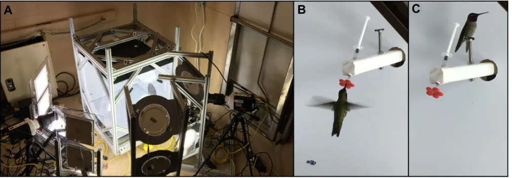
Fig. 1. Aerodynamic force platform setup at low-noise field station.(A) The aerodynamic force platform (AFP) is supported by an 80/20 Inc. aluminium frame with acrylic side walls; the enclosure allows the bird to fly freely and offers clear optical access for lights and high-speed cameras. (B) Close-up photo of an

Anna’s hummingbird hovering in front of the feeder. (C) Close-up photo of an Anna’s hummingbird inside the chamber, showing how the bird sits on the

instrumented perch between feedings. Low-heat LED lights illuminated white vinyl stickers to provide contrast for image processing.

Journal

of

Experimental

Two additional Nano 43 sensors measured forces on the artificial flower as well as the perch (Fig. 2B,C) to determine the bird’s weight (averaged over 0.2 s before and after each flight while the bird was resting). The average rms noise level in the force measured before takeoff was 4.5 mN (9.4% of body weight) for the AFP and 4.2 mN (8.7% of body weight) for the instrumented perch. The noise is due to ambient background noise and is close to sensor resolution (2 mN). The average absolute difference between the unloaded AFP before and after the flight was 1.2 mN (2.5% of body

weight) while the average difference between the perch forces was 0.8 mN (1.7% of body weight). These are a factor of two lower than sensor resolution (2 mN) and are therefore inconsequential (differences may be caused by hummingbird urination and sensor drift). Vertical forces were filtered offline (8th order digital low-pass Butterworth filter with cut-off frequency of 180 Hz;∼4.4 times the wingbeat frequency; unfiltered traces shown as light colors in Fig. 2C–F). The 180 Hz cut-off frequency was chosen to filter out the natural frequencies of the AFP, which were obtained by

B

A

C

D

E

F

Perch force Aerodynamic

force

–3 –2 –1 0 1 2 3 4

–50 0 50 100 150 200

Whole-flight force (mN)

Down Up

0 0.05 0.1 0.15 0.2 0.25

0 0.05 0.1 0.15 0.2 0.25

0 0.05 0.1 0.15 0.2 0.25

–50 0 50 100 150

T

op plate (mN)

–50 0 50 100 150

Bottom plate (mN)

Time (s) –50

0 50 100 150

Net vertical force (mN)

F2(t)

F1(t) F3(t) Bottom plate forces

F5(t) F4(t) F6(t) Top plate forces

Force sensors Top force plate

Bottom force plate High-speed

cameras

Perch forces F7(t)

F8(t) Weight F(t)

Pressure waves

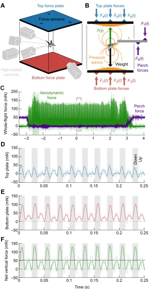
Fig. 2. Vertical aerodynamic force of a hummingbird measured_{in vivo}with an AFP.(A) The platform and five 3D-calibrated high-speed cameras simultaneously recorded aerodynamic forces and wing kinematics (artificial flower not shown). (B) The pressure field generated by the hummingbird travels to the boundaries of the flight volume at the speed of sound. The top and bottom plate mechanically integrate the pressure distribution, which is measured by three force sensors on each plate. The perch and feeder are both mounted on an instrumented carbon fiber beam that measures the weight of the

bird during takeoff and landing.F, force;t, time. (C) Combined,

the perch and aerodynamic forces represent the time-resolved (180 Hz cut-off filter) vertical momentum transfer of the bird to the earth. The bracketed region is shown on an enlarged scale in

D–F, as the force measured on the top plate (D) and bottom plate

(E), and the net vertical force (F) with the bird’s weight in black

during 10 wingbeats (shaded area, downstroke; light colors are raw measurements before low-pass filtering).

Journal

of

Experimental

measuring the impulse response of the system. The structural natural frequencies were measured by tapping the top and bottom plate with a stiff carbon fiber rod (Fig. 3A–D). A comparison of the frequency spectrum of the force trace generated by a hummingbird and the structural natural frequency spectrum of the AFP is shown in Fig. 3E. The large peak near twice the wingbeat frequency of ∼79 Hz demonstrates that the downstroke and upstroke each generate a vertical force pulse (which doubles the number of force extremes within a beat and thus the frequency).

High-speed filming

Five high-speed cameras, four grayscale Phantom Miro M310 and one color Phantom Miro LC310 (Vision Research, Wayne, NJ, USA), were synchronized and positioned around the flight chamber as shown in Figs 1A and 2A. After the bird hovered in front of the feeder, the cameras (2000 Hz; 490μs exposure; 1280×800 pixel resolution) were post-triggered, resulting in flight recordings (Fig. 4) of 8310 frames (∼4 s). Camera-ready signals were also sent to the DAQ (USB-6210, National Instruments, Austin, TX, USA) to synchronize forces and kinematics. In total, five high-speed recordings of each bird were taken while it was hovering at the feeder.

3D camera calibration

The high-speed cameras were 3D calibrated by sweeping a wand with two black spheres at a fixed distance (2.99 mm diameter at 43.70 mm distance apart) through the volume horizontally and vertically. A single black sphere was also dropped through the volume to define the gravitationalz-axis direction. A direct linear transformation (DLT) calibration was performed using easyWand5 (Hedrick, 2008), which resulted in wand quality scores of 0.40, 0.58, 0.59, 0.37, 0.63, 0.57 and 0.53 (a score of less than 1 indicates a good calibration) (Hedrick, 2008; Theriault et al., 2014).

Automated wingbeat segmentation for calculating average force within a beat

We determined the average vertical aerodynamic force trace during a wingbeat by analyzing stationary hovering flight at the feeder (Movie 1). Steady hovering flight was defined as the bird hovering at the feeder with its bill in the artificial flower, which we automatically detected with a custom-written MATLAB (R2015b, MathWorks, Sunnyvale, CA, USA) script. We excluded the first

three and last three wingbeats at the feeder to ensure stationary hovering. Wingbeat transitions were also determined automatically by tracking the horizontal position of the centroid of the birds’ silhouettes (side view, Movie 2). These video data were used to segment the force measurements and automatically identify the individual force trace for each wingbeat. Next, the average vertical force trace was determined for a wingbeat, which was subsequently normalized with the average weight of the bird (as measured by the perch). Upstroke weight support was calculated by integrating the vertical aerodynamic force trace over the upstroke and dividing it by

A

B

267 Hz

Time (s) –1.5

0 1.5

Force (N)

260 Hz

0 100 200 300 400 500 0 100 200 300 400 500 Frequency (Hz)

0 100 200 300 400 500

Normalized power

0 1 2 3 4

0 1 2 3 4

–1.5 0 1.5

39 Hz

79 Hz

Superimposed tapping structural frequencies

180 Hz low-pass

filter

Normalized power from hummingbird

C

D

E

Fig. 3. The natural frequencies of the AFP are above 250 Hz.The natural frequencies were determined by tapping the top (A) and bottom (B) plate with a stiff carbon fiber rod to obtain the frequency responses (C and D, respectively). The frequency spectrum from 132 consecutive wingbeats of bird 2 (E) shows how the wingbeat is mostly composed of a 39 and 79 Hz pulse signal (green). A 180 Hz low-pass filter was selected to cut out the system vibrations (gray area from

C and D) while preserving the hummingbird_’s force signal (green).

A

B

C

D

E

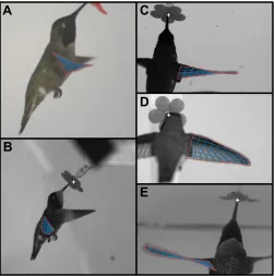
Fig. 4. Projection of the linearly twisted hummingbird wing model in five cropped camera views.(A–E) We manually positioned a 3D twisted wing in such a way that the calibrated projection best fitted each camera view (custom MATLAB script and GUI). The red lines indicate the wing outline, the blue lines indicate the twisted span and chord gridlines, and the white crosses indicate the estimated reference position of the flower. The view in C illustrates how the wing twist parameter allowed the projected wing to closely match actual wing

shape during extreme twist (frame shows the beginning of the upstroke).

Journal

of

Experimental

the integral of vertical aerodynamic force over the entire wingbeat (upstroke impulse/total wingbeat impulse). Further, we calculated the flapping frequency, the relative duration of the downstroke and the total weight support for each wingbeat (Table S1). When we applied the maximum and minimum stroke angle definition for wingbeat transition, it did not change the transitions more than one frame (∼2% of wingbeat period) or upstroke weight support percentage more than 1% (tracking the kinematics of five wingbeats per bird). Finally, we determined the normalized weight support trace within a complete wingbeat for all six hummingbirds; for this, we first interpolated every force sample to 1000 samples per wingbeat, then calculated the average force trace (Fig. 5A) over the wingbeats (n=568–789) of all birds (N=6), totaling 4094 wingbeats. Average values for each bird are given in Table S1.

Wing kinematics measurement

We determined the kinematics of the right wing by selecting and analyzing five wingbeats from each bird (N=6 birds;n=5 wingbeats per bird; 30 wingbeats total). From each of the five independent flight recordings per bird, one wingbeat was randomly selected from a subset of wingbeats that matched the average wingbeat frequency. Next, we projected a 3D linearly twisted planform of the right wing of the bird in the five camera views (Fig. 4) using the DLT calibration (Hedrick, 2008) (custom MATLAB GUI). The 3D representation of the wing was defined by seven parameters and best fitted across all five views by hand. Three parameters defined the 3D position (x,y,z) of the wing, and three Euler angles defined the rotation about thex-,y- andz-axes. The seventh parameter defined linear twist about the long axis of the wing. These seven parameters were manually adjusted to best fit the twisted and projected hummingbird wing outline in all five camera views. Finally, we filtered the manually tracked wing kinematics parameters with a 4th order digital low-pass Butterworth filter with a cut-off frequency of 400 Hz (∼10 times the wingbeat frequency).

Wing kinematics parameters

The measured wing kinematics were converted to the standard decomposition of wing stroke, deviation and angle of attack (Sane and Dickinson, 2001) (Fig. 6A,C). We improved the description of wing kinematics by including linear wing twist (Fig. 6B,C), considering the kinematics of 100 blade element segments (Dickson et al., 2008; Leishman, 2006) (see Appendix, Fig. A1) and by determining the projected vertical‘actuator disk’area of the wing (Fig. S1). The wing planform (Fig. 4) fitted well throughout the wingbeat cycle, because the upstroke to downstroke span ratio is approximately constant for hovering hummingbirds (Tobalske et al., 2007). The wing tip location was used to calculate the stroke and deviation angle with respect to the horizontal stroke plane. We determined the orthogonal stroke and deviation angular velocities using the ‘perfect smoother’ developed by Eilers (2003). This smoother optimized the time derivatives we needed to determine the wing angular velocity vector (see Appendix, Fig. A1A). Eilers’ smoother (Eilers, 2003) was also used to determine the wing angular acceleration vector (see Appendix, Fig. A1B). Subsequently, we divided the wing planform into 100 wing segments, equally spaced down the span of the wing along the midline. The wing’s angular velocity and acceleration vectors were crossed with the position vector of each wing segment to obtain the local velocity and acceleration over the wingbeat (see Appendix, section A2). The local aerodynamic angle of attack of the wing was defined as the angle between the chord vector and the wing velocity vector. The chord vector at each spanwise wing element pointed from the

midspan line to the leading edge of the wing. As the wing is twisted, the angle of attack varied along the span (see Appendix, Fig. A1C). Because the wing is inverted on the upstroke, the angle of attack with respect to the wing was negative (Kruyt et al., 2014). This inversion allowed us to use an angle of attack-specific drag

A

C

0 50 100

–1 0 1 2 3

In vivo

hummingbird weight support

0 50 100

–1 0 1 2 3

In vivo

parrotlet weight support

0 50 100

Wingbeat cycle (%) –1

0 1 2 3

Robofly

Drosophila

weight support

0 50 100

–1 0 1 2 3

CFD hawkmoth weight support

28±1

6 50

24

0 15 30 45 60

Upstroke weight support (%)

1.25 ±0.03

1.35 1.29

1.26

1 1.1 1.2 1.3 1.4

T

e

mporal cost factor

B

D

E

F

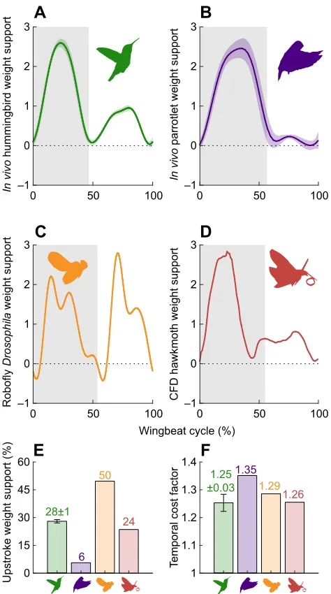
Fig. 5. More equally distributed weight support decreases induced power penalty in hummingbirds,_Drosophilaand hawk moths, compared with that of parrotlets.(A) Wingbeat-resolved vertical aerodynamic force during

the downstroke (shaded area) and upstroke of Anna’s hummingbird (N=6

birds;n=568–789 wingbeats per bird; light green, s.d.). (B) Wingbeat-resolved

vertical aerodynamic force during the downstroke (shaded area) and upstroke

of a Pacific parrotlet (adapted from Chin and Lentink, 2017;N=4 birds;

light purple, s.d.). (C) Wingbeat-resolved vertical aerodynamic force during

the downstroke (shaded area) and upstroke ofDrosophilabased on

measurements with a robot fly model (adapted from Muijres et al., 2014). (D) Wingbeat-resolved vertical aerodynamic force for a hawk moth calculated

via computational fluid dynamics simulations based onin vivowing shape and

kinematics measurements (adapted from Zheng et al., 2013). (E) Anna’s

hummingbirds support bodyweight during the upstroke, more than a generalist

parrotlet, but not symmetrically likeDrosophila. (F) Hummingbirds, fruit flies

and hawk moths incur a lower induced power penalty, represented by the temporal cost factor (see Appendix, Eqn A1f ), than parrotlets, thanks to a more even distribution of weight support over the wingbeat (error bars, s.d., across N=6 hummingbirds).

Journal

of

Experimental

coefficient for both the downstroke and upstroke (see Fig. S2 and Appendix, section A3). The angle of attack was ill defined at stroke reversal, because wing velocity approached zero. We therefore calculated the instantaneous local rotational velocity (see Appendix, Fig. A1D) using the rotational velocity of the root and tip of the

wing (see Appendix, Eqn A4e), which accounted for angular velocity caused by wing twist and eliminated error caused by the velocity singularity. Finally, we calculated the area swept by the wing by creating a point cloud based on the position of the wing outline over the whole stroke. These points were projected into the horizontal stroke plane, which we used to calculate the vertical

‘actuator disk’area of the right wing shown in Fig. S1 (using an

‘alpha hull’ with a probe radius of 10 mm in a custom-written MATLAB script). To also account for the left wing, we multiplied the actuator disk area by a factor of two.

Force and power model for hovering flight

A quasi-steady wing element model (Sane and Dickinson, 2002; Dickson et al., 2008; Song et al., 2015) was used to estimate the instantaneous aerodynamic force (Fig. 6D,E) and power (Fig. 6F,G). The aerodynamic force calculation included translational lift and drag components, as well as rotational and added mass forces (Fig. 6D; see Appendix, section A4). Drag contributed to vertical weight support, because the stroke plane is

U-shaped, which points the drag force out of the horizontal plane. Translational lift and profile drag calculations were based on wing spinner force measurements with preparedC. annawings (Kruyt et al., 2014) (Fig. S2A). Rotational force was calculated with our measured wing rotational velocity in combination with a rotational force coefficient derived based on the axis of rotation of a hummingbird wing (Song et al., 2015) (see Appendix, Eqn A4c). Finally, the added mass force was calculated based on flat plate theory (Dickson et al., 2008; Sedov, 1980) in combination with our measured wing acceleration (see Appendix, Eqn A4f ). We integrated the vertical force contributions over all 100 spanwise wing elements. Aerodynamic torque (Fig. 7) was calculated by crossing the aerodynamic force at each blade element with its radial position from the shoulder (see Appendix, section A8). A similar quasi-steady wing element model was developed to calculate the aerodynamic power needed to hover (Fig. 6F,G). This model included profile, induced, rotational and added mass power (see Appendix, section A5). Compared with earlier experimental studies, we improved the profile and induced power calculations as follows: we calculated profile power by separating measured translational drag (Kruyt et al., 2014) into its induced and profile drag components, so that we could use profile drag coefficient as a function of angle of attack to calculate profile drag and power (Fig. S2B; see Appendix, Eqn A3b), instead of assuming a constant profile drag coefficient (Ellington, 1984; Chai and Dudley, 1995, 1996; Altshuler et al., 2010a). As our unique experimental setup measures vertical forcein vivo, we were also able to calculate the induced power (Leishman, 2006) by using the actual vertical force generated by the hummingbird (Fig. 5A). Aerodynamic power due to rotation and added mass were calculated by dot multiplying the forces with the local wing velocity vector and integrating them for all wing elements over the whole stroke, which was similar to the force calculation above. Inertial power is calculated based on wing mass and radius of gyration for C. anna wings (Fig. 6G; see Appendix, section A7). We determined the body mass-specific power (Fig. 6F,G) by dividing the power by the mass of each bird, and the muscle mass-specific power (Fig. 8) by dividing the power by the mass of the associated flight muscle. Each muscle was defined to be involved from the moment the power dropped below zero through its storage phase and release until the power once again dropped below zero as shown in Fig. 8B. This definition agrees with the EMG firing and muscle tension traces (Fig. 7D) as well as the sign of the torque (Fig. 7B). We adopted EMG traces from the

A

C

D

E

F

G

Stroke

Deviation Angle of

attack

Twist

0 50 100

Wingbeat cycle (%)

0 50 100

0 50 100

Wingbeat cycle (%)

0 50 100

0 50 100

Wingbeat cycle (%) –90 –60 –30 0 30 60 90

Wing kinematic angle (deg)

Lift

Drag Rotational

Added mass

–0.5 0 0.5 1 1.5 2

Quasi-steady weight support

Total aero

–0.5 0 0.5 1 1.5 2

Profile

Induced

Rotational

Added mass

–25 0 25 50 75 100

Body mass-specific power (W kg

–1)

Aero

Inertial

Aero + inertial

–150 –75 0 75 150 225 Flat wing

–Stroke

DeviationAngle of_attack

Twist

B

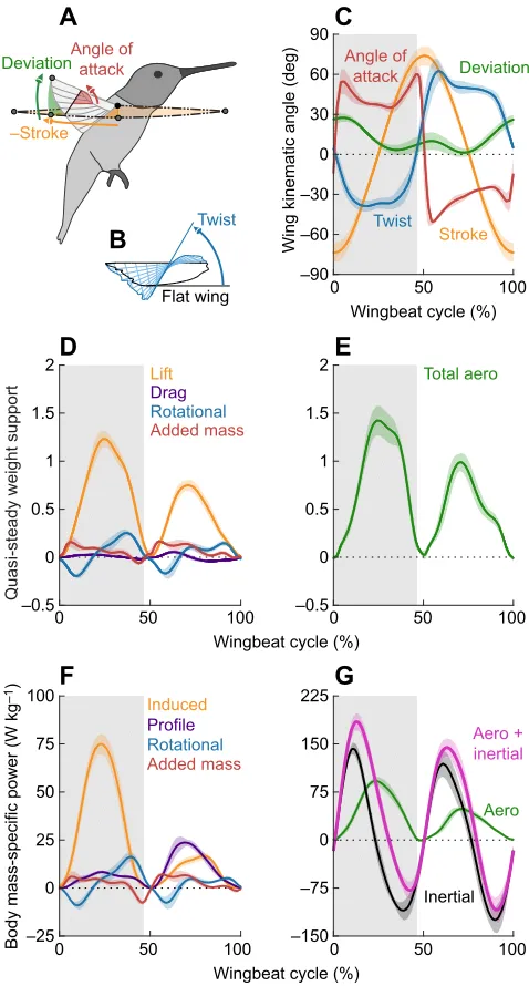
Fig. 6. The aerodynamic power required to hover is smaller than the inertial power required to beat the wing.(A,B) Definitions of the measured wingbeat kinematics for the aerodynamic force and power model (stroke is

shown in the negative direction). (C) The measured (N=6 birds;n=5 wingbeats

per bird; light colors, s.d.; shaded area is downstroke) wing stroke, deviation, twist (tip relative to root) and angle of attack (at the center of pressure where

torque due to drag acts on the wing,^r3¼0:56). (D) Predicted vertical lift, drag,

rotational and added mass force components that support bodyweight show that translational lift makes the greatest contribution. (E) The quasi-steady model under-predicts weight support (64%) and over-predicts aerodynamic symmetry of the hummingbird compared with the directly measured vertical force (Fig. 5A). (F) The induced, profile, rotational and added mass power components, divided by body mass, show that induced power is the largest aerodynamic power component. (G) Total body mass-specific power is driven by wing inertia, which switches from positive to negative. This can be reconciled by a spring that efficiently stores high instantaneous negative power for elastic recoil.

Journal

of

Experimental

pectoralis and supracoracoideus (Fig. 7D) measured for Anna’s hummingbirds (Altshuler et al., 2010b), because these measurements were also made for hovering flight. Whereas these particular EMG signals are representative for hovering Anna’s hummingbirds, flight muscle EMG traces have multiple peaks during maximal load-lifting trials in Anna’s hummingbirds (Altshuler et al., 2010b) and may vary somewhat between species (Tobalske et al., 2010). Combined, the two flight muscles represent approximately 25% of the hummingbird’s body mass (Chai and Dudley, 1995, 1996), with the pectoralis and supracoracoideus representing approximately 17% (Clark, 2009) and 8%, respectively. Models and calculations are presented in full detail in the Appendix.

RESULTS

An active upstroke allows for efficient hovering

Our instantaneous force measurements show that Anna’s support 28±1% of their bodyweight during the upstroke (Fig. 5A; N=6

birds;n=568–789 wingbeats per bird). Upstroke weight support is thus appreciable but asymmetric in hummingbirds as previously estimated based on flow measurements (Warrick et al., 2005, 2009; Wolf et al., 2013) and CFDs models (Song et al., 2014, 2015). Comparing thein vivohummingbird (Fig. 5A) andin vivoPacific parrotlet (Chin and Lentink, 2017) (Fig. 5B) force measurements, we see that hummingbirds generate appreciably more weight support during the upstroke than generalist birds in slow or hovering flight. Whereas hummingbirds also generate more upstroke support than hawk moths (Fig. 5D), they do not generate as much upstroke support as fruit flies (Fig. 5C). On average, we measure 99±3% of the vertical aerodynamic force that Anna’s hummingbirds need to support their bodyweight in flight. We derived simple aerodynamic theory (see Appendix, section A1) to show how generating more equally distributed weight support over the wingbeat reduces the induced power requirements. Because of the non-linearity of the induced power equation, minor deviations from generating constant vertical force have small effects, while larger deviations have an increasingly greater induced power penalty (in the form of a temporal cost factor; see Appendix, Eqn A1e; Fig. 5F). This explains why we find that hummingbirds incur a somewhat lower penalty (1.25±0.03) than Drosophila (1.29), because weight support fluctuates more in Drosophila, whereas both incur a lower cost than the Pacific parrotlet (1.35). Overall, the hummingbird induced power penalty is similarly low in hummingbirds, Drosophila and hawk moths, compared with that in Pacific parrotlets (Fig. 5F). This mechanistically underpins why hummingbirds converged closer towards generating more upstroke weight support, relative to their generalist bird ancestors (McGuire et al., 2014), to reduce the cost of sustained hovering flight.

Quasi-steady model predicts high inertial requirements

The quasi-steady aerodynamic force model (Fig. 6;N=6 birds;n=5 wingbeats per bird) for Anna’s hummingbirds accounts for 64±4% of bodyweight support and predicts that the upstroke contributes 39±1% to the total quasi-steady vertical force (Fig. 6E). Stroke-averaged vertical force is composed of∼84% translational lift,∼0% translational drag, ∼5% rotational force and ∼11% added mass force (Fig. 6D). Our detailed 3D kinematic wing model showed that hummingbird wings twist up to −38 deg during the downstroke and up to 62 deg during the upstroke (Fig. 6C). Dynamic changes in wing twist affects both the magnitude and radial distribution of rotational and added mass forces acting on the wing during pronation and supination. The model’s capacity to predict most of the weight support in hummingbirds is similar to predictions forDrosophila(Dickinson et al., 1999; Dickson et al., 2008) but below 100% because of additional effects not captured by a quasi-steady model. Therefore, aerodynamic power must also be underestimated, because induced power is proportional to vertical aerodynamic force to the power of 1.5 (see Appendix, Eqn A1b). To overcome these underestimates (Weis-Fogh, 1972; Chai and Dudley, 1995; Kruyt et al., 2014), as well as the over-prediction of upstroke weight support, we calculated the induced power (Fig. 6F) directly based on the measuredin vivovertical force (Fig. 5A). The total aerodynamic power consists of∼63% induced power, while profile power represents ∼23%. The power due to rotational force and to added mass force is relatively small,∼7% and ∼7%, respectively (Fig. 6F). In total, Anna’s hummingbirds need a stroke-averaged aerodynamic power of 35±1 W kg−1_{of body mass,}

with peak values of ∼100 W kg−1 _{(Fig. 6G). Whereas these}

sustained power values are amongst the highest reported for skeletal

A

B

C

D

Supra (aero + inertial) Aero

Inertial

Pect (aero + inertial)

0 50 100

Wingbeat cycle (%) –50

–25 0 25 50

Bodyweight-specific torque (mm)

Supra (aero + inertial)

Upstroke start Downstroke

start

Pect (aero + inertial)

Aero Inertial

–90 –45 0 45 90 Stroke angle (deg) –50

–25 0 25 50

Bodyweight-specific torque (mm)

22.7 Hz 52.5 Hz

0 50 100

Wingbeat cycle (%) 0

2 4 6 8

Pect muscle force (

g

)

Pect EMG Supra EMG

x y

z

z-acceleration

z-torque

Wingtip path

T

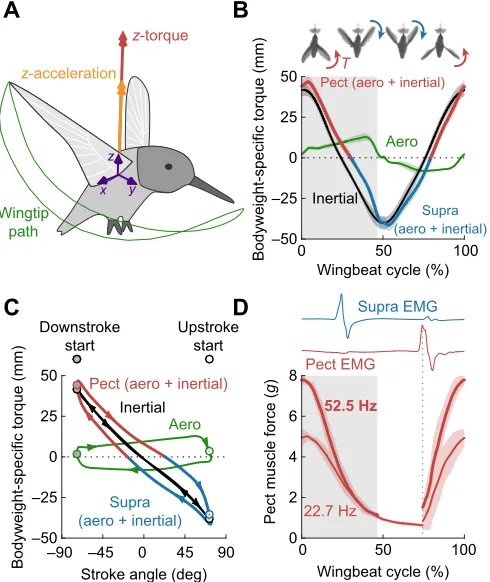
Fig. 7. The pectoralis coordinates upstroke to downstroke reversal, whereas the supracoracoideus coordinates downstroke to upstroke reversal.(A) Definition of positive wing torque and acceleration in the vertical (z) direction. (B) The net vertical (z) torque (T; aerodynamic+inertial) required to flap the right wing reaches extrema during stroke reversal. Following the torque sign convention (A), positive torque must be generated by the pectoralis (Pect) pull and negative torque by the supracoracoideus (Supra) pull at stroke reversal. This is consistent with the antagonistic arrangement of these flight muscles (shaded area is downstroke). (C) The effect of wing inertia dominating aerodynamic drag is that it tilts the wing aero-mechanical torque loop. With elastic recoil, the torque loop would primarily feed aerodynamic dissipation while recoil overcomes wing inertia. (D) The pectoralis and supracoracoideus are activated roughly a quarter of a wingbeat period before stroke reversal in

Anna’s hummingbirds (EMG adapted from Altshuler et al., 2010b) and the

pectoralis reaches peak isometric force about 8 ms after activation (muscle

force adapted from Hagiwara et al., 1968). Thein situmuscle force

development lines up with the corroborated peak wing torque (B) with light red regions representing s.d. across all force peaks at each stimulus frequency

(see Fig. S3).

Journal

of

Experimental

muscle, even more power is needed to overcome wing inertia at stroke reversal (Wells, 1993b). With the inertia added, the hummingbird flight muscles, the pectoralis and supracoracoideus, need to deliver a peak power of almost 200 and 150 W kg−1_{of body}

mass, respectively, to beat the wings back and forth. This power value cannot be explained with existing theories unless elastic storage in the flight apparatus is assumed (Weis-Fogh, 1972; Chai and Dudley, 1995, 1996; Ellington, 1984; Wells, 1993b) (Fig. 6G).

DISCUSSION

Wing inertia determines muscle activation timing

To better understand hummingbird muscle function, we calculated (see Appendix, section A8) the net torque around the shoulder joint, wingbeat resolved based on wing drag and inertia (Fig. 7A). The net torque switches direction at midstroke for both flight muscles, because wing inertia is high and the aerodynamic drag is insufficient to decelerate the wing (Fig. 7B). The antagonistic flight muscle pair has to generate the instantaneous net torque needed to overcome wing inertia and drag, which forms an aero-mechanical torque loop throughout the wingbeat (Fig. 7C). The effect of wing inertia dominating aerodynamic drag is that it tilts the torque loop, as predicted based on first principles by Weis-Fogh (1972). This causes wing torque to peak at stroke reversal, instead of midstroke, and dictates the effective work that the pectoral and supracoracoideus muscle–tendon units need to deliver together. This‘internal’net muscle-generated torque×angular displacement has to be equal to (or larger than) the ‘external’ net wing torque×angular displacement (depending on friction and other internal losses; Weis-Fogh, 1972). We can determine which muscle–tendon unit has to perform which effective work, because the pectoralis delivers the net torque (muscle force×lever arm) required for upstroke to downstroke reversal, while the supracoracoideus coordinates downstroke to upstroke reversal. The antagonistic flight muscle pair must accommodate this peak inertial torque requirement to reverse the stroke direction. The pectoralis (main downstroke muscle; Altshuler et al., 2010b; Tobalske et al., 2010; Donovan et al., 2012; Mahalingam and

Welch, 2013) is the primary muscle that can pull to generate the positive braking torque required to coordinate the upstroke to downstroke reversal. Similarly, the supracoracoideus (main upstroke muscle; Altshuler et al., 2010b; Tobalske et al., 2010; Donovan et al., 2012; Mahalingam and Welch, 2013) has to be activated well before the start of the upstroke to generate the negative braking torque required for downstroke to upstroke reversal (Fig. 7B). Indeed, it has been shown (Altshuler et al., 2010b; Donovan et al., 2012) that Anna’s hummingbirds activate the pectoralis and supracoracoideus a quarter of a wingbeat in advance of the upstroke–downstroke and downstroke–upstroke transition, respectively (Fig. 7D)–approximately a quarter-stroke earlier than found in other birds (Altshuler et al., 2010b; Tobalske et al., 2010; Mahalingam and Welch, 2013). The activation appears to be well timed, because Hagiwara et al. (1968) found that the pectoralis of Anna’s hummingbirds reaches peak isometric force in under 8 ms after activationin situ, regardless of whether it is activated by a single pulse (twitch) or a pulse train at 23 or 53 Hz [a range that encompasses Anna’s hummingbird wingbeat frequency of 41 Hz, although Hagiwara et al. (1968) even showed noticeable force peaks with tetanus from stimulations of up to 300 Hz; Fig. S3]. Comparing the time to peak isometric force of Anna’s hummingbirds (8 ms; 4.9 g body mass) with values for the Etruscan shrew extensor digitorum longus (11 ms; 1.8 g body mass), the fastest mammal locomotory muscle recorded to date (Peters et al., 1999; Jürgens, 2002), it becomes clear that scaling effects cannot fully explain the speed of Anna’s hummingbird pectoralis muscle. It is reasonable to assume the pectoralis and supracoracoideus are similarly fast in Anna’s hummingbirds, because the fiber type of both flight muscles is uniformly fast oxidative glycolytic (Donovan et al., 2012; Welch and Altshuler, 2009). These fibers enable Anna’s hummingbird pectoralis to reach peak force faster than the so-called‘superfast’ muscles that control the dove’s trill (Elemans et al., 2004). Superfast muscles in other animals are not generally known to be primary motors for locomotion (Fuxjager et al., 2016), because they generate low specific power at high frequencies (Elemans et al., 2004, 2008; Fuxjager et al., 2016; Rome, 2006). Similar early activation in frog

A

B

C

D

Storage Storage

Pect

Supra

–30 0 30 60 90 –30 0 30 60 90 –30 0 30 60 90

Wingbeat cycle (%) –1000

–500 0 500 1000 1500 2000

Downstroke start

Pect

Extension

Contraction

Stroke angle (deg) 0

10 20 30 40 50

Bodyweight-specific torque (mm)

Upstroke start Supra

Extension

Contraction

0 10 20 30 40 50

Pect Supra

Pect

Perfect elastic storage

Supra

Zero elastic storage 0

100 200 300 400

Muscle mass-specific power (W kg

–1

)

500

n 40

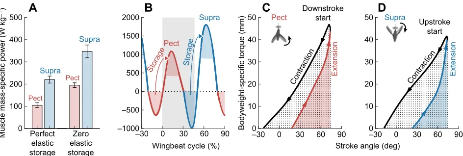
Fig. 8. Negative work during wing deceleration has to be stored and released elastically to hover efficiently.(A) Wingbeat-averaged power requirements for the pectoralis and supracoracoideus muscles are almost halved by storing elastic energy as the wing decelerates before stroke reversal, and then releasing it to accelerate the wing again. (B) Instantaneous muscle mass-specific power requirements over a wingbeat show how this negative power can be stored and released to decrease the high instantaneous power peaks. We shifted and lengthened the wingbeat cycle axis for clarity; the gray area represents

the downstroke. The muscle–tendon units of the pectoralis (C) and supracoracoideus (D) first have to extend as the wing decelerates, before contracting to

accelerate the wing again. These muscle contractions and forces drive the external wing stroke angles and torques we determined, which shape the aero-mechanical muscle work loop (C,D). Arrows over hummingbird avatars show the direction of positive bodyweight-specific torque and stroke angle in the reference frame of each muscle. Elastic recoil can efficiently absorb and release the substantial negative work due to wing inertia. The negative work is shown by the red and blue colored areas, while the partially overlapping positive work is shown by the black dotted area.

Journal

of

Experimental

muscle–tendon units corresponds to a more spring-like work loop that stores elastic energy, albeit imperfectly (Sawicki et al., 2015). Assuming isometric muscle measurements are a reasonable approximation to estimate the time between activation and peak muscle forcein vivo, we find that the resulting peak muscle force measured by Hagiwara et al. (1968) (Fig. 7D) aligns with the peak torque (muscle force×moment arm) demand at stroke reversal that we calculated (Fig. 7B). It would require a further 6 ms delay (¼ wingbeat) in muscle force development due to contractile kinetics for the muscle peak to instead coincide with maximum wing velocity, much longer than the 2 ms uncertainty we found in the definition of stroke reversal. Whereas torque peaks at stroke reversal, power demand (Fig. 6G) is approximately zero, because wing angular velocity reaches zero. This is consistent with the near-zero instantaneous strain rate in the pectoralis muscle (low power) at stroke reversal in Rufous hummingbirds (Tobalske et al., 2010).

Recoil in the flight apparatus explains peak instantaneous power

In the absence of elastic storage, a hummingbird would have to generate 195±11 and 347±29 W kg−1 _{of muscle mass in the}

pectoralis and supracoracoideus, respectively (averaged over a full wingbeat, assuming negative power is free; Fig. 8A). By storing all negative power elastically and releasing it to accelerate the wing again, the hummingbird would only have to generate 105±11 and 220±16 W kg−1_{of power in the pectoralis and supracoracoideus,}

respectively (Fig. 8A). Weis-Fogh and Alexander (1977) estimated the theoretical maximum is about 250 W kg−1_{muscle mass based}

on hummingbirds’ physiological limits, while Pennycuick and Rezende (1984) estimated it to be as high as 430 W kg−1_muscle

mass. Josephson (1993) suspected these are overestimates due to unrealistic muscle contractile parameter assumptions and a failure to account for activation/inactivation time. Although these power outputs are already very high for vertebrates, the flight muscles are capable of delivering over three times more profile power (Altshuler et al., 2004) during maximum load-lifting trails (Chai and Millard, 1997; Altshuler et al., 2004; Skandalis et al., 2017). Using additional load-lifting data from Anna’s hummingbirds (Altshuler et al., 2010b; Segre et al., 2015), we confirm this estimate and calculate that the induced and inertial power also triple during burst muscle performance (see Appendix, section A10). Further, the nominal instantaneous total power peaks in hovering hummingbirds are between 1000 and 2000 W kg−1_{muscle mass for each muscle}

(Fig. 8B), exceeding peak power during burst takeoff in quail (1121 W kg−1_{; Askew and Marsh, 2001) and matching peak power}

in projecting chameleon tongues, which use elastic storage to achieve it (1892 W kg−1_{; Anderson and Deban, 2010). It is}

therefore more parsimonious to assume peak power is achieved by releasing stored elastic energy, especially because this extraordinary power output has to be sustained over many thousands of contraction cycles during foraging flight. Whereas physiological limits do not enable muscles to deliver such high power over so many cycles, springs can generate extreme instantaneous power with similar double frequency traces using near-zero work per cycle. Another way to visualize the opportunity for elastic storage in hummingbirds is to plot the aero-mechanical torque loop in the reference frame of each muscle. During forward flight, a generalist starling (at 13.7 m s−1_{; Biewener et al., 1992),}

magpie (at 6 m s−1_{; Dial et al., 1997), budgerigar (at 4 m s}−1_;

Ellerby and Askew, 2007) and pigeon during slow flight (at 3.9 m s−1_{; Tobalske and Biewener, 2008) have a relatively upright}

pectoralis work loop with minimal negative work during the end of

the upstroke. The supracoracoideus, however, generates more negative work, which may be stored elastically in the supracoracoid tendon (Tobalske and Biewener, 2008). In contrast, the torque loop of hovering hummingbirds is tilted as a result of high wing inertia, allowing a larger area of negative work while decelerating the wing (Fig. 8C,D). They can efficiently store the high instantaneous negative work and release it again as positive work via elastic recoil (Roberts et al., 1997; Dickinson et al., 2000; Biewener, 2003). Elastic energy can be stored in tendons (Mahalingam and Welch, 2013; Alexander, 2002) and the muscle itself (Alexander and Bennet-Clark, 1977; Dickinson et al., 2000; Sawicki et al., 2015). Finally, because wing inertia dominates aerodynamics and our predictions for inertial effects are grounded in established dynamics theory (see Appendix, Fig. A2 and section A9), our understanding of how hummingbirds use elastic recoil to tune their wingbeat are robust to aerodynamic modeling errors.

Conclusion

Our analysis shows that hummingbirds andDrosophila are about equally aerodynamically efficient based on the induced power required to sustain hovering. Further, three lines of wingbeat-resolved evidence show that the most parsimonious explanation for the extreme instantaneous performance of the hummingbird flight apparatus is elastic recoil. Only recoil can reconcile (i) the instantaneous peak torque at stroke reversal (Fig. 7B), which requires exceptional muscle work, with (ii) the early activation (Altshuler et al., 2010b; Donovan et al., 2012) and fast contractile dynamics (Hagiwara et al., 1968) of Anna’s hummingbird flight muscle (Fig. 7D), and (iii) the peak instantaneous power of well over 1000 W kg−1 _{for each flight muscle–tendon unit (Fig. 8B), in}

concert. Overall these findings support Weis-Fogh’s hypothesis that Drosophilaand hummingbirds must have converged on similarly low induced power and inertial cost to sustain hovering. The finding that recoil is critical to overcome the inertia of flapping wings at low energetic cost in hummingbirds shows how current bird-sized flapping aerial robots (Lentink et al., 2009; Keennon et al., 2012) could be made dramatically more energy efficient by adding a spring in their flap. Future studies can build upon these results by exploring the diversity in the flight apparatus of birds (Tobalske, 2016) and bats (Riskin et al., 2012; Konow et al., 2017), both in laboratory settings and in more realistic, ecological settings with animals entering the platform voluntarily to feed (see ruggedized platform in Movie 3).

APPENDIX

Our hummingbird aerodynamics models and equations developed here integrate and expand the existing quasi-steady aerodynamics model for insect flight (Dickson et al., 2008) and the blade element model for rotorcraft (Leishman, 2006).

A1: induced power penalty

To determine how hummingbirds would benefit from supporting bodyweight symmetrically within a wingbeat, we considered the downward acceleration of air through the stroke plane that generates a vertical force (Leishman, 2006; Ellington, 1984; Chai and Dudley, 1995; Weis-Fogh, 1972). The resulting high-velocity wake below the bird has increased momentum and kinetic energy. The increase in kinetic energy requires‘induced’power,Pind, delivered by the

flight muscles to the wings and is proportional to vertical force raised to the power of 1.5. This cost function intuitively shows that it is more efficient to generate constant thrust throughout the stroke because any decrease in vertical force during one part of the

Journal

of

Experimental

wingbeat will need to be compensated for by an equivalent increase in force during another part of the wingbeat, which will cost more power than is saved. We expanded the corresponding‘actuator disk’ theory (Leishman, 2006; Chai and Dudley, 1995; Weis-Fogh, 1972; Norberg, 2012) to determine the analytical fitness function that relates the actual average induced power, Pind, to the theoretical

minimum induced power,Pind;min, as a function of instantaneous

weight support over the wingbeat. The average induced power,Pind,

was calculated (Leishman, 2006; Ellington, 1984) by multiplying the robot or animal’s weight, W, by the velocity of the induced flow,vind:

vind¼ ffiffiffiffiffiffiffiffi

W 2rA

s

; ðA1aÞ

whereρis the density of air andAis the area swept by the wings. This allowed us to describePindas:

Pind¼k

ffiffiffiffiffiffiffiffi

W3

2rA

s

; ðA1bÞ

whereκis the induced power factor that accounts for tip losses, non-uniform inflow and other non-ideal effects (Leishman, 2006). A value of κ=1.2 is typically assumed for bird flapping flight (Norberg, 2012; Pennycuick, 2008; Tobalske et al., 2003). Ellington (1984) broke this induced power factor up into a spatial correction factor,σ, and a temporal correction factor,τ:

k_¼1þsþt: ðA1cÞ

Given we measured the temporal distribution of the vertical force directly, we can quantify the additional penalty that an animal incurs by generating a time-varying wake. To decouple, we defineκσto be the spatial cost factor (withκ_σ=1 corresponding to a uniform wake) andκτto be the temporal cost factor (withκτ=1 corresponding to a constant wake). Using Ellington’s estimates (Ellington, 1984), we assume a value of σ=0.1, which leads to κσ=1.1. We can then describe the ideal average induced power as:

Pind;ideal¼ ffiffiffiffiffiffiffiffi

W3

2rA

s

ðA1dÞ

and the induced power including losses due to temporal force fluctuation as:

Pind;temp¼

1 T

ðT

0

Pind;tempðtÞdt¼

1 T

ðT

0 ffiffiffiffiffiffiffiffiffiffiffi

FðtÞ3 2rA

s

dt; ðA1eÞ

whereTis the wingbeat period andF(t) is the aerodynamic vertical force, which must be equal to the animal’s weight on average to enable sustained hovering. The induced power cost due to time-varying vertical force can be quantified by calculating the ratio with the ideal induced power:

kt¼

Pind;temp

Pind;ideal¼

1 T

ðT

0 ffiffiffiffiffiffiffiffiffiffiffi

FðtÞ3 W3 s

dt¼1 T

ðT

0 FðtÞ

W

1:5

dt: ðA1fÞ

This cost factor is equal to 1 ifF(t)=W, but will be greater than 1 if the vertical force varies during the wingbeat. As we measured the termF(t)/W in vivo, we can directly calculate the induced power factor that the animal incurs. The calculated induced power temporal cost factor for Anna’s hummingbirds, parrotlets, Drosophilaand hawk moths is shown in Fig. 5F.

A2: wing element velocity and acceleration

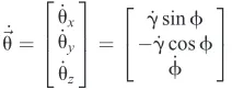
For our aerodynamic force and power model, we calculated radial force distribution, which depended on the wings’radial velocity and acceleration distribution, calculated below. Letφbe the stroke angle and γ be the deviation angle of the right wing as defined in Fig. 6A. We used Eilers’perfect smoother (Eilers, 2003) to calculate the derivatives of the stroke and deviation angle with respect to time,

_

f and g_. The resultant wing angular velocity vector,~u_, with componentsu_x,u_y andu_zis:

_

~u_¼ _ u_x _ u_y

_ u_z

2 6 4

3 7

5¼ _

gsinf

g_cosf

_ f

2 4

3

5_{: ð}A2aÞ

These three components are plotted in Fig. A1A. The derivative of the wing angular velocity vector with respect to time,~u€, with components €u_x, €u_yand €u_z, was again determined using Eilers’

A

B

C

D

x

y

z

0 50 100 0 50 100

Wingbeat cycle (%)

0 50 100 0 50 100

–2 –1 0 1 2

Angular velocity (

×10

4 deg s

–1

)

x

y

z

–6 –4 –2 0 2 4 6

Angular acceleration (×10

6 deg s

–2

)

Root

Tip

–90 –60 –30 0 30 60 90

Angle of attack (deg)

Root

Tip –3

–2 –1 0 1 2 3

Rotational velocity (×10

4 deg s

–1

)

Fig. A1. Wingtip and radial angle of attack kinematics for bird 2.(A) The three components of the wing_’s angular velocity vector show that the vertical component (z) was largest, because it defined velocity in the horizontal stroke plane. (B) The angular acceleration vector for the wing was calculated as the derivative of the angular velocity vector: again, the vertical component (z) was largest because it defined acceleration in the horizontal stroke plane. (C) The angle of attack varied from the wing root to the tip because the wing was twisted spanwise relative to the incoming velocity. (D) As a result of dynamic wing twist, the rotational velocity of the wing also varied spanwise. The angle of attack and the associated rotational velocity are shown for five of 100 equally spaced wing elements.

Journal

of

Experimental

perfect smoother (Fig. A1B). We then calculated the angular velocity and acceleration vector of each wing element by estimating the wing element position vector in space,~pe, as follows:

~pe¼re

cosfcosg sinfcosg

sing

2 4

3

5_{; ð}A2bÞ

where reis the distance to each wing element. This allowed the

velocity,~ue, at each element to be calculated by:

~ue¼~u_~pe ðA2cÞ

and the acceleration,~ae, to be calculated by:

~ae¼~u€~pe: ðA2dÞ

A3: profile drag coefficient

We improved upon existing drag calculations (Ellington, 1984; Chai and Dudley, 1995, 1996; Altshuler et al., 2010a) by determining the profile drag coefficient as a function of angle of attack. For this, we used the measured lift,CL, and drag,CD, coefficients of spinning C. annawings from Kruyt et al. (2014) (Fig. S2A) in whichCD

included both profile and induced drag as a function of angle of attack. Based on these coefficients, we separated the total drag power into its induced (see Appendix, Eqn A1b) and profile components as follows:

21 2rð^r3RÞ

3

SCDðaÞf_3¼k

ffiffiffiffiffiffiffiffi

F3 2rA

s

þ21

2rð^r3RÞ

3

SCD;profðaÞf_ 3

;

ðA3aÞ

where the vertical force isF ¼ 21 2rð^r2RÞ

2

S Ck LðaÞkf_2,Ris the wing radius,^r2and^r3 are the second and third moments of area

(Kruyt et al., 2014), andSis the surface area of the wing. Replacing Fand rearranging this equation to get an expression forCD,prof, we

obtained:

CD;profðaÞ ¼CDðaÞ

k_ðr_ð^r2RÞ2SkCLðaÞ kf_ 2

Þ3=2

r_ð^r3RÞ3Sf_

3 ffiffiffiffiffiffiffiffi

2rA p

¼CDðaÞ k ^_^r2

r3

3 ffiffiffiffiffiffi

S 2A

r

ðkCLðaÞ kÞ3=2: ðA3bÞ

We next substituted the specific wing geometry parameters from Kruyt et al. (2014) (^r2¼0:50, r^3¼0:55, S=680 mm2, A=7260 mm2_{), and assumed (Norberg, 2012; Pennycuick, 2008;}

Tobalske et al., 2003)κ=1.2, to calculate the profile drag coefficient as a function of angle of attack (Fig. S2B).

A4: quasi-steady vertical force

To calculate the instantaneous vertical force, we used a quasi-steady model for flapping animal flight (Dickson et al., 2008; Song et al., 2015; Dickinson et al., 1999). This model predicted the translational, rotational and added mass forces on each wing element over the wingbeat, of which we took the vertical components. The translational lift force of each wing element was:

FL;e¼

1

2rcek~uek

2

CLðaeÞDr; ðA4aÞ

whereceis the chord length of the wing element,Δris the width of

the element andαeis the angle of attack of the element. Similarly,

the translational profile drag force of each wing element was calculated by:

FD;e¼

1

2rcek~uek

2

CD;profðaeÞDr: ðA4bÞ

The induced drag is assumed to act perpendicular to the induced flow, so does not contribute to the vertical force. The rotational force at each wing element was calculated by (Dickson et al., 2008):

FR;e¼Crrvece2k~uekDr; ðA4cÞ

whereCris the rotational force coefficient andωeis the rotational

velocity of each element. The theoretical value for the rotational force coefficient was calculated by (Dickson et al., 2008; Fung, 2008; Sane and Dickinson, 2002):

Cr¼pð0:75^x0Þ; ðA4dÞ

where^x0is the non-dimensional axis of rotation. Song et al. (2015)

calculated an average value of^x0¼0:453 for five representative chord locations for hovering ruby-throated hummingbird kinematics. We rounded this value to^x0¼0:5 (which represents the estimated accuracy of this number forC. anna) to calculate the rotational force coefficient for Anna’s hummingbirds in our study, Cr=0.8. To determine the rotational force, we calculated the

rotational velocity, ωe, by first finding the rotational velocity of the wing base,ωb, and then the rotational velocity of the wing tip with respect to the base due to wing twist,ωt. The rotational velocity at each wing element (Fig. A1D) was then:

ve ¼vbþre

Rvt; ðA4eÞ

whereRis the radius of the wing. The added mass force at each wing element was thus calculated as:

FA;e¼ rp_c2

e

4

~ue~ae

k~uek

sinðaeÞþ k~uekvecosðaeÞ

D_{r: ð}A4 fÞ

This term accounted for the additional air the wing had to accelerate as it flapped. The rotational and added mass forces acted normal to the back surface of the wing. As the wing was twisted, this normal vector changed with the radial position of the wing element. We accounted for wing twist in our vertical force calculation, which sums up the vertical component of the translational, rotational and added mass forces in a custom-written MATLAB script.

A5: quasi-steady power model

We extended existing aerodynamic power models (Song et al., 2015; Ellington, 1984; Chai and Dudley, 1995, 1996; Altshuler et al., 2010a; Norberg, 2012) with an improved calculation of profile and induced power to estimate the instantaneous power required to hover. The profile power at each wing element,PP,e, was calculated

by:

PP;e ¼

1

2rcek~uek

3

CD;profðaeÞDr; ðA5aÞ

where CD,prof is the profile component of the drag coefficient

calculated above (see Appendix, Eqn A3b) and plotted in Fig. S2B. The instantaneous induced power was calculated more precisely by substituting the measuredin vivovertical force in established actuator disk theory (Leishman, 2006; Ellington, 1984; Chai and Dudley, 1995, 1996; Altshuler et al., 2010a; Norberg, 2012). The induced

Journal

of

Experimental

power for both wings combined,PI(t), was thus calculated as:

PIðtÞ ¼ks ffiffiffiffiffiffiffiffi

1 2rA

s

FðtÞ1:5: ðA5bÞ

The rotational and added mass power required at each wing element were calculated by dot multiplying the force vectors by the incoming air velocityð~ueÞ:

PR;e¼ ~ue~FR;e ðA5cÞ

PA;e¼ ~ue~FA;e: ðA5dÞ

To get the total instantaneous aerodynamic power,Paero(t), we

summed the power contribution from each wing element, multiplied by 2 to account for the two wings, and added the induced power based on thein vivomeasured vertical force:

PaeroðtÞ ¼2X

e

PP;eðtÞ þ2

X

e PR;eðtÞ

þ2X

e

PA;eðtÞ þPIðtÞ: ðA5eÞ

The calculation of induced power based on in vivo force measurement allows us to quantitatively estimate the total instantaneous aerodynamic power.

A6: simplified wingbeat-averaged aerodynamic power estimate

To determine how our stroke-resolved measurements compared to previous stroke-averaged actuator disk models, we analyzed the former and determined the stroke averaged profile drag coefficient and induced power cost factor needed to match our power results. The average profile power for one wing,PP, was estimated by:

PP¼

1 T

ðT

0

1

2rSCD;profjv

3_ðtÞjdt

¼1

T

ðT

0

1 2rð^r3RÞ

3

SCD;profjf_ 3

ðtÞjdt

¼1

2rð^r3RÞ

3 SCD;prof

1 T

ðT

0

jf_3_ðtÞjdt: ðA6aÞ

whereCD;prof is the average profile drag coefficient,v(t) is the wing

velocity,^r3is the third moment of area andf_ðtÞis the stroke angular

velocity. By assuming a harmonic stroke, we can write:

f_ðtÞ ¼ Fcosð2pftÞ; ðA6bÞ _

f_ðtÞ ¼F2pfsinð2pftÞ; ðA6cÞ

whereΦ(in radians) is the stroke amplitude (half of the total swept stroke angle) andfis the wingbeat frequency (1/T). The integral then becomes:

ðT

0

jf_3

ðtÞjdt¼ ðF2pfÞ3

ðT

0

jðsinð2pftÞÞ3jdt¼32

3 F

3_p2

f2 ðA6dÞ

and the average profile power over the wingbeat for one wing is:

PP¼

16p2 3 rð^r3RÞ

3

SCD;profF3f3: ðA6eÞ

We found that a value for CD;prof of 0.16 best matched our

stroke-averaged high-fidelity profile power calculation. This equation is similar to the one derived by Ellington (1984) with the exception that the stroke is assumed to be harmonic, which approximates hummingbirds well (Fig. 6C). The average induced power,PI, for the bird can be calculated based on the weight,W, and

the actuator disk area swept by the wing, A=2 ΦR2_{. If vertical}

force is assumed to be equal to weight throughout the stroke, the power will be underestimated. To correct for this, we use the spatial and temporal cost factors introduced above (see Appendix, section A1):

PI¼kskt

ffiffiffiffiffiffiffiffi

W3

2rA

s

: ðA6fÞ

We use κσ=1.1 and κτ=1.25 to best match our stroke-averaged high-fidelity induced power calculation. As profile and induced power alone make up 86% of the modeled total aerodynamic power,

Paero, we approximated the aerodynamic power without detailed

kinematics as:

Paero2PPþPI

¼32₃p2r_ð^r3RÞ

3

SCD;profF3f3þkskt ffiffiffiffiffiffiffiffi

W3 2rA

s

: ðA6gÞ

A7: inertial power

The inertial power needed to accelerate and decelerate the wing is often ignored in insect studies, because a mechanism for elastic storage has been identified in the thorax that can cancel inertial power out. It is still unknown how and with what efficiency hummingbirds can store elastic energy during their wingbeat. To determine the physiological consequences of different elastic storage scenarios, we calculated inertial power. Inertial power, Pinertial, is the dot product of the wing torque and angular velocity,~u_

(Fig. A1A). Torque is the moment of inertia about the wing base,I, times the angular acceleration,~u€(Fig. A1B). The inertial power of one hummingbird wing is thus:

PinertialðtÞ ¼Ið~u€ðtÞ ~u_ðtÞÞ: ðA7aÞ The moment of inertia of the wing can be calculated by dividing the wing into small chord strips and measuring their masses,mi, and

distances,ri, from the wing base:

I¼Xmir2i: ðA7bÞ

The non-dimensional radius of gyration,^r2ðmÞ, is defined such that:

Idefmwð^r2RÞ2; ðA7cÞ

wheremwis the mass of one wing andRis the wing length. Using

the following equation, we calculated an^r2ðmÞvalue (0.265) using the radial distance and mass of 10 wing chord strips from a male Anna’s hummingbird (Ortega-Jimenez and Dudley, 2012) (N=1):

^

r2ðmÞ ¼ 1 R

ffiffiffiffiffiffiffiffiffiffiffiffiffiffiffi P

mir2i P

mi s

: ðA7dÞ

As a second measure, we calculated the non-dimensional ^r2ðmÞ value for another species of hummingbird (Amazilia fimbriata fluvaitilis) based on Weis-Fogh’s inertial wing measurements. By combining Weis-Fogh’s (1972) published wing moment of inertia,

Journal

of

Experimental