warwick.ac.uk/lib-publications
Original citation:
Sprittles, James E. and Shikhmurzaev, Yulii D.. (2013) Finite element simulation of dynamic
wetting flows as an interface formation process. Journal of Computational Physics, 233 . pp.
34-65.
Permanent WRAP URL:
http://wrap.warwick.ac.uk/78931
Copyright and reuse:
The Warwick Research Archive Portal (WRAP) makes this work by researchers of the
University of Warwick available open access under the following conditions. Copyright ©
and all moral rights to the version of the paper presented here belong to the individual
author(s) and/or other copyright owners. To the extent reasonable and practicable the
material made available in WRAP has been checked for eligibility before being made
available.
Copies of full items can be used for personal research or study, educational, or not-for-profit
purposes without prior permission or charge. Provided that the authors, title and full
bibliographic details are credited, a hyperlink and/or URL is given for the original metadata
page and the content is not changed in any way.
Publisher’s statement:
© 2013, Elsevier. Licensed under the Creative Commons
Attribution-NonCommercial-NoDerivatives 4.0 International
http://creativecommons.org/licenses/by-nc-nd/4.0/
A note on versions:
The version presented here may differ from the published version or, version of record, if
you wish to cite this item you are advised to consult the publisher’s version. Please see the
‘permanent WRAP URL’ above for details on accessing the published version and note that
access may require a subscription.
Finite Element Simulation of Dynamic Wetting Flows as an Interface
Formation Process
J.E. Sprittlesa1and Y.D. Shikhmurzaevb
aMathematical Institute, University of Oxford, Oxford, OX1 3LB, U.K.
bSchool of Mathematics, University of Birmingham, Edgbaston, Birmingham, B15 2TT, U.K.
Abstract
A mathematically challenging model of dynamic wetting as a process of interface formation has been, for the first time, fully incorporated into a numerical code based on the finite element method and applied, as a test case, to the problem of capillary rise. The motivation for this work comes from the fact that, as discovered experimentally more than a decade ago, the key variable in dynamic wetting flows — the dynamic contact angle — depends not just on the velocity of the three-phase contact line but on the entire flow field/geometry. Hence, to describe this effect, it becomes necessary to use the mathematical model that has this dependence as its integral part. A new physical effect, termed the ‘hydrodynamic resist to dynamic wetting’, is discovered where the influence of the capillary’s radius on the dynamic contact angle, and hence on the global flow, is computed. The capabilities of the numerical framework are then demonstrated by comparing the results to experiments on the unsteady capillary rise, where excellent agreement is obtained. Practical recommendations on the spatial resolution required by the numerical scheme for a given set of non-dimensional similarity parameters are provided, and a comparison to asymptotic results available in limiting cases confirms that the code is converging to the correct solution. The appendix gives a user-friendly step-by-step guide specifying the entire implementation and allowing the reader to easily reproduce all presented results, including the benchmark calculations.
Keywords: Fluid Mechanics, Dynamic Wetting, Interface Formation, Shikhmurzaev Model, Computation, Capillary Rise
1. Introduction
Reliable simulation of flows in which a liquid advances over a solid, known as dynamic wetting flows, is the key to the understanding of a whole host of natural phenomena and technological processes. In the technological context, the study of these flows has often been motivated by the need to optimizecontinuous
coating processes that are routinely used to create thin liquid films on a product [1], for example, in the coating of optical fibres [2, 3]. However, more recently, discrete coating, in particular inkjet printing of microdrops [4], has matured into a viable, and often preferable, alternative to traditional fabrication processes, e.g. in the additive manufacturing of 3D structures or the creation of P-OLED displays [5, 6], and it is becoming a new driving force behind research into dynamic wetting phenomena. In most cases, such flows can be regarded as microfluidic phenomena, where a large surface-to-volume ratio brings in interfacial effects on the flow that are not observed at larger scales.
Obtaining accurate information about micro and nanofluidic flows experimentally is often difficult and usually costly so that, consequently, a desired alternative is to have a reliable theory describing the physics
1Corresponding author.
Email address: a [email protected] and b [email protected](J.E. Sprittlesa and Y.D.
Shikhmurzaevb)
that is dominant for this class of flows and incorporate it into a flexible and robust computational tool which can quickly map the parameter space of interest to allow a specific process to be optimized. Such computational software could be validated against experiments at scales and geometries easily accessible to accurate measurement and then used to make predictions in processes inaccessible to experimental analysis. The discovery that no solution exists for the moving contact-line problem in the framework of standard fluid mechanics [7, 8] prompted a number of remedies to be proposed, which are summarized, for example, in [ch. 3 of 9]. Of these, most are what we shall refer to as ‘conventional’ or ‘slip’ models, in which the no-slip condition on the solid surface is relaxed to allow a solution to exist, with the Navier-slip condition [10] being the most popular choice. As a boundary condition on the free-surface shape at the contact line, one has to specify the contact angle formed between the free surface and solid. In conventional models, this angle is prescribed as a heuristic or empirical function of the contact-line speed and material parameters of the system, e.g. [11, 12]. Such models provide predictions that adequately describe experiments at relatively large scales, often around the length scale of millimetres. It is well established that on such scales many of the proposed models work equally well and that finding significant deviations between their predictions, and hence ascertaining which best captures the key physical mechanisms of dynamic wetting, is practically impossible [13, 14].
A physical phenomenon that gives an opportunity to distinguish between different models came to be known under a ‘technological’ name of the ‘hydrodynamic assist of dynamic wetting’ (henceforth ‘hydrody-namic assist’ or simply ‘assist’). The essence of this effect, first observed in high accuracy experiments on the curtain coating process [15, 16], is that for a given liquid spreading over a given solid at a fixed contact-line speed, the dynamic contact angle can still be manipulated by altering the flow field/geometry, for example, in the case of curtain coating, by changing the flow rate or the height from which the curtain falls. This effect has profound technological implications as it allows the process to be optimized by off-setting the increase of the contact angle with increasing contact-line speed by manipulating the flow conditions and hence postponing air entrainment [15].
The dependence of the dynamic contact angle on the flow field has also been reported in the imbibition of liquid into capillaries [17, 18], in the spreading of impacted drops over solid substrates [19, 20] and in the coating of fibres [3]. However, in many of these flows it is yet unclear whether hydrodynamic assist actually occurs, or whether the free surface bends significantly beneath the spatial resolution of the experiments, whereas for curtain coating the hope of attributing assist to the poor spatial resolution of experiments has been quashed by careful finite element simulations which show that the degree of free-surface bending under the reported resolution of the measurements is too small to account for the observed effect and that conventional models cannot in principle describe this important physical effect [21].
Currently, the only model known to be able to even qualitatively describe assist [22, 23] is the model of dynamic wetting as an interface formation process, first introduced in [24] and discussed in detail in [9]. This model is based on the simple physical idea that dynamic wetting, as the very name suggests, is the process in which a fresh liquid-solid interface (a newly ‘wetted’ solid surface) forms. Qualitatively, the origin of the hydrodynamic assist is that the global flow influences the dynamics of the relaxation of the forming liquid-solid interface towards its equilibrium state and hence the value of this interface’s surface tension at the contact line, which, together with the surface tension on the free surface, determines the value of the dynamic contact angle. When there is a separation of scales between the interface formation process and the global flow, the ‘moving contact-line problem’ can be considered locally and asymptotic analysis provides a speed-angle relationship which is seen to describe experiments just as well as formulae proposed in other models [9]. However, in the situation where the scale of the global flow and that of the interface formation are no longer separated, the influence of the flow field on the dynamic contact angle will occur and hence no unique speed-angle relationship will be able to describe experiments. Then, the interface formation model becomes the only modelling tool, and, given that the processes of practical interest are free-surface flows under the influence of, at least, viscosity, capillarity and inertia, it is inevitable that, to describe such flows, one needs computer simulation, i.e. the development of accurate CFD codes, which, for the effect of hydrodynamic assist to be captured, have to incorporate the interface formation model.
especially on the microscale. Review articles have also referred to the description of assist using this model as one of the main challenges in the field [26]. The major obstacle in the development of this computational tool is the mathematical complexity of the interface formation model, as one has to solve numerically the Navier-Stokes equations describing the bulk flow subject to boundary conditions which are themselves partial differential equations along the interfaces and in their turn have to satisfy certain boundary conditions at contact lines confining the interfaces. These conditions determine the dynamic contact angle and hence influence the free-surface shape, which exerts its influence back on the bulk flow. Thus, the bulk flow, the distribution of the surface parameters along the interfaces and the dynamic contact angle that these distributions ‘negotiate’ become interdependent, with the dynamic contact angle being an outcome of the solution as opposed to conventional models where it is aninput. This interdependency is, on the one hand, the physical essence of the experimentally observed effect of hydrodynamic assist to be described but, on the other hand, it is this very interdependency that, coupled with the nonlinearity of the bulk equations and the flow geometry, is the reason why the model is difficult to implement robustly into a numerical code.
Some numerical progress has been made for the computationally less complex steady Stokes flows [23], but what is lacking is a step-by-step guide to the implementation of this model in the general case, with unsteady effects in the bulk and interfaces as well as nonlinearity of the bulk equations fully implemented. This which would pave the way for incorporating the interface formation model into existing codes as well as developing new ones. Therefore, the first objective of the present paper is to address these issues and provide a digestible guide to the model’s implementation into CFD codes. Then, after giving benchmark computational results to verify this implementation, we consider a problem of imbibition into a capillary, compare the outcome with experiments and predict essentially new physical effects.
A starting point in the development of the aforementioned CFD code is to first develop an accurate computational approach for the simulation of dynamic wetting flows using the mathematically less complex conventional models and this was achieved in [27]. It was shown that many of the previous numerical results obtained for dynamic wetting processes are unreliable as they contain uncontrolled errors caused by not resolving all the scales in the conventional model, most notably the dynamics of slip and the curvature of the free surface near the contact line. Benchmark calculations in [27] for a range of mesh resolutions resolved previous misunderstandings about how to impose the dynamic contact angle and showed that implementing it using the usual finite element ideology, as opposed to ‘strong’ implementation of the contact angle, works most efficiently: it allows errors to be seen, and hence controlled, as the computed contact angle varies from its imposed value, instead of them being masked elsewhere in the code. Furthermore, in [28], we have shown that numerical artifacts which occur at obtuse contact angles are present in both commercial software and in academic codes where, misleadingly, they have previously been interpreted as physical effects. By comparing computational results to analytic near field asymptotic ones, we have shown that the previously obtained spikes in the distributions of pressure observed near the contact angle are completely spurious, and, to rectify this issue a special method, based on removing the ‘hidden’ eigensolutions in the problem prior to computation, has been developed [28]. In [29], we showed that our code is capable of simulating unsteady high deformation flows by comparing to benchmark calculations published in the literature and performed by various research groups. In contrast, in [30] it has been shown that when commercial software is used to simulate relatively simple benchmark free surface flows, the converged solution is not the correct one.
flows of interest where interface formation or disappearance also occurs is a straightforward procedure computationally, and it will be dealt with in forthcoming articles.
The layout of the present article is as follows. First, in §2, without limiting ourself to a particular flow configuration, the equations describing the dynamic wetting process are briefly recapitulated. Then, in§3, the finite element equations are derived for the dynamic wetting flow as an interface formation process. Local element matrices, and additional details about the finite element procedure are provided in the Appendix, which complements a ‘user-friendly’ step-by step guide to finite element simulation given for this class of flows in [27] and allows one to reproduce the benchmark simulations in§4. These simulations are performed for the dynamic wetting flow through a capillary both in the case where the meniscus motion is steady and for the unsteady imbibition of a liquid into an initially dry capillary. Computations are checked for convergence both as the mesh is refined and towards asymptotic results in limiting cases. Having established the accuracy of our approach, in§5 new physical effects are discovered by considering the influence of capillary geometry on the dynamic wetting process. Finally, the computational tool’s ability to easily describe experimental data is shown in§6 and a number of advantages over current approaches, particularly in the initial stages of a meniscus’ motion into a capillary tube, are highlighted. Concluding remarks and areas for future research are discussed in§7.
2. Modelling dynamic wetting flows as an interface formation process
Consider the spreading of a Newtonian liquid, with constant densityρand viscosityµ, over a chemically homogeneous smooth solid surface. The liquid is surrounded by a gas which, for simplicity, is assumed to be inviscid and dynamically passive, of a constant pressurepg. Let the flow be characterized by scales for lengthL, velocityU, timeL/U, pressureµU/Land external body forceF0. In the dimensionless form, the
continuity and momentum balance equations are then given by
∇ ·u= 0, Re
∂u
∂t +u· ∇u
=∇ ·P+St F, (1)
where
P=−pI+h∇u+ (∇u)Ti, (2)
is the stress tensor,t is time,uandpare the liquid’s velocity and pressure, Fis the external force density and I is the metric tensor of the coordinate system. The non-dimensional parameters are the Reynolds numberRe=ρU L/µand the Stokes numberSt=ρF0L2/(µU).
Boundary conditions to the bulk equations are required at the liquid-gas free surface x =x1(s1, s2, t),
whose position is to be found as part of the solution, and at the liquid-solid interfacex=x2(s1, s2, t), whose
position is known, and at other bounding surfaces which will be specified by the problem of interest; here, (s1, s2) are the coordinates that parameterize the surfaces. Boundary conditions along the free surface, the
liquid-solid interface and the contact line at which they intersect are provided by the interface formation model [9], as follows.
2.1. The interface formation model
To represent the boundary conditions on an interface with a normalnin an invariant form, it is convenient to introduce a (symmetric) tensorI−nn, which is essentially a metric tensor on the surface. If an arbitrary vectorais decomposed into a scalar normal componentan=a·nand a vector tangential parta||, so that a=a||+ann, we can see that, becausen·(I−nn) =0, the tensor (I−nn) extracts the component of a vector which is tangential to the surface, i.e.a·(I−nn) =a||. Hereafter,nis the unit normal to a surface pointingintothe liquid, and subscripts 1 and 2 refer to the free surface and solid surface, respectively.
The equations of interface formation on a liquid-gas free surface, which act as boundary conditions for the bulk equations (1), are given by
∂x
1 ∂t −v
s
1
Can1·
h
∇u+ (∇u)Ti·(I−n1n1) +∇σ1=0, (4)
Canpg−p+n1·
h
∇u+ (∇u)Ti·n1
o
=σ1∇ ·n1, (5)
vs1||−u||=
1 + 4 ¯αβ¯
4 ¯β ∇σ1, (6)
(u−vs1)·n1=Q(ρs1−ρ
s
1e), (7)
∂ ρs
1
∂t +∇ ·(ρ
s
1v
s
1)
=−(ρs1−ρs1e), (8)
σ1=λ(1−ρs1), (9)
whilst at liquid-solid interfaces formed on a solid which moves with velocity U, the equations of interface formation have the form
(vs2−U)·n2= 0, (10)
Can2·P·(I−n2n2) +12∇σ2= ¯β u||−U||
, (11)
vs2||−1
2 u||+U||
= ¯α∇σ2, (12)
(u−vs2)·n2=Q(ρs2−ρ
s
2e), (13)
∂ ρs
2
∂t +∇ ·(ρ
s
2v
s
2)
=−(ρs2−ρs2e), (14)
σ2=λ(1−ρs2). (15)
The differential term σ1∇ ·n1, where σ1 is the (dimensionless) surface tension on the free surface,
describing the capillary pressure in the normal-stress equation (5) indicates that this equation requires its own boundary condition where the free surface terminates, i.e. at the contact line. Theren2is known andn1
must be specified by setting the dynamic contact angleθd at which the free surface meets the solid surface:
n1·n2=−cosθd. (16)
This angle is determined from a force balance at the contact line, given by Young’s equation [31]:
σ2+σ1cosθd=σS, (17)
where σ2 and σS are the surface tensions of the liquid-solid interface and solid-gas interface, respectively, and the latter is henceforth assumed to be negligibleσS ≈0. Equations (8) and (14) also require a boundary condition at the contact line where the two interfaces meet, and here we have the continuity of surface mass flux
ρs1vs1||−Uc
·m1+ρs2
vs2||−Uc
·m2= 0 (18)
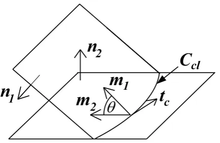
where Uc is the (dimensionless) velocity of the advancing contact line and mi is the inward unit vector tangential to surfaceiand normal to the contact line (see Figure 1).
The interface formation model is described in detail in the monograph [9] and a series of preceding papers [e.g. 24, 32] so that here only the main ideas are briefly recapitulated. The surface variables are in the ‘surface phase’, i.e. physically in a microscopic layer of liquid adjacent to the surface which is subject to intermolecular forces from two bulk phases. In the continuum limit, this microscopic layer becomes a mathematical surface of zero thickness withρsdenoting its surface density (mass per unit area) andvsthe velocity with which it is transported. The following non-dimensional parameters have been introduced ¯α=ασ/(U L), ¯β = (βU L)/σ,
= U τ /L, λ=γρs
(0)/σ and Q=ρ
s
(0)/(ρU τ) which are based on phenomenological material constants α, β, γ, τ andρs
(0); in the simplest variant of the theory, the latter are assumed to be constant and take the
Figure 1: Illustration showing the vectors associated with the liquid-gas free surfaceA1 and the liquid-solid surfaceA2 in the
vicinity of the contact lineCcl.
Estimates for the material constants have been obtained by comparing the theory to experiments in dynamic wetting, e.g. in [33], but could just as easily have been taken from an entirely different process in which interface formation is key to describing the dynamics of the flow [34, 35, 36, 37]. In other words, once obtained for a particular liquid in one set of experiments, the material constants determined can be used to describe all phenomena involving the same fluid in which interface formation dynamics ‘kicks in’.
The surface tension σi is considered as a dynamic quantity related to the surface density ρsi via the equations of state in the ‘surface phase’ (9) and (15), which are taken here in their simplest linear form. Gradients in surface tension influence the flow, firstly, via the stress boundary conditions (4), (5) and (11), i.e. via the Marangoni effect, and, secondly, in the Darcy-type equations3(6) and (12) by forcing the surface
velocity to deviate from that generated in the surface phase by the outer flow. Mass exchange between the bulk and surface phases, caused by the possible deviation of the surface density from its equilibrium value
ρs
e, is accounted for in the boundary conditions for the normal component of bulk velocity (7) and (13), and in the corresponding surface mass balance equations (8) and (14).
One would expect a generalized set of boundary conditions to have the classical conditions as their limiting case. For the interface formation model this limiting case follows from the double limit→0, β/Ca¯ → ∞. When the limit→0 is applied to (3)–(9), the liquid-gas interface equations are reduced to their classical form. Notably, if we apply →0 to the liquid-solid equations (10)–(15), the conventional ‘slip’ model is obtained, that is the Navier-slip condition combined with impermeability. In this limit, the surfaces are in equilibrium so Young’s equation (17) gives that the dynamic contact angle is fixed as a constant at its equilibrium valueθd=θe. If we wish to go further with the conventional model approach and describe the dynamic contact angle as some function of the contact-line speed, then Young’s equation must be discarded in favour of this function. Therefore, implementing the interface formation model into a numerical code allows one to test all conventional models of wetting proposed in the framework of continuum mechanics. By applying the limit ¯β/Ca(=βL/µ)→ ∞we recover the classical equations of no-slip and impermeability on the solid surface for which the moving contact-line problem is known to have no solution [7, 8].
Despite the model’s complexity, in limiting cases, analytic progress on it can be made to obtain explicit relationships for the surface variables and, with some further assumptions, even a formula relating the contact-line speed to the dynamic contact angle. Such formulae are a useful test of our numerical solutions, and we will briefly recapitulate their outcome.
3The analogy with the Darcy equation is that the tangential surface velocityvs
2.2. Asymptotic formulae in a limiting case
When the contact-line motion can be analyzed as a local problem, as opposed to cases where the interface formation and the bulk flow scales are not separated so that manipulating the global flow influences the relaxation process along the interfaces, asymptotic progress is possible. A full derivation of the results we use may be found in [9] and references therein; here we shall just outline the main assumptions and results. If in the steady propagation of a liquid-gas free surface over a solid substrate in the Stokes regime (Re1), the characteristic length scale of the interface formation processl=U τ is small compared to the bulk length scaleL, we have that our non-dimensional parameter1. If in the limit→0 we also assume that the capillary numberCa→0, then, to leading order inCa, the normal-stress boundary condition (5) gives that the free surface near the contact line is planar, so that the problem may be considered locally in a wedge-shaped domain. Then, we can identify the following three asymptotic regions:
(a) The outer region, where, in a reference frame moving with the contact line, one has a flow in a wedge in the classical formulation, with a zero tangential-stress and a no-slip boundary, described in [38]; (b) The intermediate region with the characteristic (dimensionless) length scale , where the
surface-tension-relaxation process takes place and where, due to smallness ofCa, to leading order the influence of the bulk flow on this process can be neglected;
(c) The inner region, with the characteristic length scale Ca, through which the surface densities and velocities, to leading order, stay constant.
On the free surface, at leading order in the intermediate and inner regions, one has
ρs1=ρs1e, v1s||=uf(θd), (19)
whereuf(θd) is the (dimensionless) radial velocity of the bulk flow in the far field on the liquid-gas interface given by [38]:
uf(θd) =
sinθd−θdcosθd sinθdcosθd−θd
, (20)
so that the surface mass flux into the contact line is −ρs1euf(θd). Then, since the surface variables are constant through the inner region, the boundary conditions at the contact line (17), (18) can be applied to the distributions of the surface variables in the intermediate region. As a result, we have two first-order ODEs to solve for the distributions ofρs
2 andv2s|| along the liquid-solid interface
dρs2
d¯s = 4V
2(1−vs
2||),
d(ρs
2v2s||)
d¯s =−(ρ
s
2−ρ
s
2e) (¯s >0) (21)
where ¯s=s/is the intermediate region’s variable andV2= ¯β/((1+4 ¯αβ¯)λ) is the non-dimensional contact-line speed, subject to (a) boundary condition (18), now taking the formρs2vs2=−ρs1euf(θd) at ¯s= 0, (b) the matching conditionρs2→ρs2eas ¯s→ ∞, and, as boundary condition (a) implicitly depends on the parameter
θd, (c) Young’s equation (17), now taking the form cosθd=λ(ρs2−1). The equilibrium contact angleθeis obviously related toρs2eby cosθe=λ(ρs2e−1), which can be used to replaceρs2e withθe.
The above problem is easily solved numerically; however, by taking an additional assumption λ 1, one can obtain an analytic relation between the contact angle and the non-dimensional speed of the contact lineV:
cosθe−cosθd =
2Vhcosθe+ (1−ρs1e) −1
(1 +ρs
1euf(θd))
i
V + [V2+ 1 + cosθ
e(1−ρs1e)]
1/2 , (22)
where
k= 2V(ρs2e)−1h V2+ρs2e1/2
−Vi, C= 2V (ρ s
2e+ρs1euf(θd))
(V2+ρs
2e)
1/2
+V .
the low-Reynolds-number region, the flow near the contact line is completely determined by the contact-line speed, and hence the mass flux into the contact line that ‘feeds’ the liquid-solid interface can be found from the local solution. This is the case considered in [24, 39], where the theory shows excellent agreement of (22) with experiments. If the outer flow is to influence the mass flux into the contact line [23], this will affect the value of the contact angle.
The most important length scaleLif associated with the interface formation process is the characteristic distance over which the solid surface returns to equilibrium and the asymptotic result indicates that this is given, in non-dimensional units, bykLif/= 1 in (19) so thatLif =ρs2e/
h 2V(p
V2+ρs
2e−V)
i .
The expressions given above will be used in §4 below to compare our computations to in the situations where the underlying assumptions of the asymptotics are satisfied. Now, we shall consider the development of this computational algorithm for the general case without making any simplifying assumptions.
3. Finite element procedure
A finite element framework for the simulation of dynamic wetting flows using the conventional models of dynamic wetting was described in [27]. To handle the evolution of the free surface this framework uses an arbitrary Lagrangian Eulerian (ALE) scheme based on the method of spines, a computational approach which has been successfully applied to a range of coating flows over the past thirty years, e.g. in [40, 41, 21]. In [29], the framework was extended for the simulation of time-dependent free surface flows, with the code providing accurate solutions for the benchmark test case [42, 43] of a freely oscillating liquid drop. This confirmed that the implementation of the viscous, inertial and capillarity effects is accurate, even when the mesh undergoesO(1) deformations.
What follows is the implementation of the interface formation equations into our framework. For a more detailed description of the basic components of the framework and a user-friendly step-by-step guide to implementing dynamic wetting flows into the finite element method, the reader is referred to [27] and in particular to the Appendix which makes it possible for the interested user to reproduce the results presented there. The Appendix in the present article provides additional details of the implementation and, in this sense, complements the Appendix in [27], allowing one to reproduce the results of§4 and§5.
3.0.1. Problem formulation in the ALE scheme
Consider how the equations of§2, written in Eulerian coordinatesx, are formulated for an ALE system where the flow domain χ = χ(x, t) deforms in time. This deformation must be accounted for in the temporal derivatives of variables whose position in the Eulerian system is evolutionary, in particular, in the Navier-Stokes equations where the material derivativeD/Dttransforms as
Du
Dt =
∂u
∂t
x
+u· ∇u= ∂u
∂t
χ
+ (u−c)· ∇u. (23)
Here, c(χ, t) = ∂x
∂t
χ
is the velocity of the ALE coordinates with respect to the fixed reference frame. It
can be seen that, as should be expected, for c=u we have a Lagrangian scheme whereas for c= 0the Eulerian system is recovered.
Before considering temporal derivatives occurring in the interface formation equations, it is convenient to introduce the surface gradient∇s, which is the projection of the usual gradient operator∇onto the surface
∇s= (I−nn)·∇. An arbitrary surface vectorasis written in terms of components normal and tangential to the surface asas=as||+asnn, whereasn=as·n, so that for its divergence one has∇ ·as=∇s·as||+a
s n∇s·n. In particular, as described in [44], points on the surfaces move with the normal surface velocity vsn, i.e. according to the kinematic equation (3), and an arbitrary tangential component cs|| which depends on the choice of mesh design. Then, on a given surface
cs=cs||+vnsn, cs||= ∂x
Therefore, in the ALE framework the left-hand side of the surface mass balance equations (8) and (14), become
∂ ρs γ ∂t xγ
+∇ · ρsγvsγ
= ∂ ρ
s γ ∂t χs γ
−csγ· ∇ρsγ+∇ · ρsγvsγ
,
where γ = 1,2 refers to the liquid-gas and liquid-solid interface, respectively, and χs
γ = χsγ(x, t) are the corresponding coordinates. Then, (8) and (14) take the form
∂ ρs
γ
∂t −c
s γ||· ∇
sρs γ+∇
s·ρs γv
s γ||
+ρsγvsγn∇s·n γ
+ρsγ−ρsγe= 0, (γ= 1,2), (24)
where we have used thatnγ· ∇sρsγ= 0. Equations (24) can be rearranged to obtain
∂ ρs
γ
∂t +ρ
s γ∇
s·cs γ||+∇
s·hρs γ
vsγ||−csγ||i+ρsγvsγn∇s·n γ
+ρsγ−ρsγe= 0, (γ= 1,2).
In the limiting case, where the surface moves only normal to itself, so that cs
γ|| =0, the usual Eulerian equations are recovered:
∂ ρs
γ
∂t +∇
s·ρs γv
s γ||
+ρsγvsγn∇s·n γ
+ρsγ−ρsγe=
∂ ρs γ
∂t +∇ · ρ
s γv s γ
+ρsγ−ρsγe= 0, (γ= 1,2),
whilst if the surface moves in a Lagrangian way, cs
γ = vsγ, then the term under the divergence becomes identically zero, and we have
∂ ρs γ
∂t +ρ
s
γ∇s·vsγ||+ρsγvsγn∇s·nγ
+ρsγ−ρsγe=
∂ ρs γ
∂t +ρ
s γ∇ ·vsγ
+ρsγ−ρsγe= 0, (γ= 1,2). (25)
Here, as should be expected, there is no term representing the convection of surface density by the surface velocity, i.e. a term of the formvs· ∇ρsdoes not appear.
Having reformulated the equations for the ALE system and introduced surface operators, we can now derive the appropriate FEM residuals.
3.0.2. Forming the finite element residuals
The defining feature of the FEM is that the computational domainV is tessellated into a finite number of non-overlapping elements, each containing a fixed number of nodes at which the functions’ values are determined. Between these nodes the functions are approximated using interpolating functions whose func-tional dependence on position is chosen. In what follows,Np is the total number of nodes inV at which the pressure is determined,Nu is the number of nodes at which the velocity components are to be found,N1is
the number of nodes on the free surfaceA1, N2 the number of nodes on the solid surface A2, and Nc the number of nodes along the contact line.
The procedure of generating the finite element equations is well known and a detailed explanation of how this is achieved for dynamic wetting flows described by the conventional model is given in [27], so that here we just give the main details. Functions are approximated as a linear combination of interpolating functions each weighted by the corresponding nodal value. In particular, we use mixed interpolation so that the Ladyzhenskaya-Babu˘ska-Brezzi [45] condition is satisfied4 with linear basis functions ψj to represent
pressure and quadratic onesφj for velocity:
p= Np
X
j=1
pjψj(x), u= Nu
X
j=1
ujφj(x), (x∈V).
In the Galerkin finite element method, the basis functions which are used to discretize the functions of the problem are also used as weighting functions to create the weak form of the problem, see [§3 of 27] for specific details. Note that here we use Roman letters for the indices (i,j, etc) to refer to the nodal values and approximating functions spanning the whole domain (globally); in the Appendix, where all the numerical details are given, these indices will be used alongside italicized ones (i, j, etc), which will refer to local, element-based, values and functions.
Surface variables are also approximated quadratically with basis functions on surface Aγ (γ = 1,2) denoted by φγ,j(s1, s2). So, all of the interface formation variables, represented by an arbitrary surface
variableas
γ, as well as the shape of the free surfacex1, are approximated as
asγ = Nγ
X
j=1
asγ,jφγ,j(s1, s2), x1=
N1
X
j=1
x1,jφ1,j(s1, s2).
To determine the free surface shape, i.e. the nodal valuesx1,j, a functionh=h(s1, s2) is found as part of
the solution at free-surface every node, so thathj=hj(s1, s2) for j = 1, ..., N1, which points in a direction
linearly independent from both s1 and s2 at each node, i.e. ‘out’ of the free surface. For example, in the
simplest case of a Cartesian coordinate system one could have the free surface at (x, y, z) = (s1, s2, h(s1, s2)),
so that h is the height above the (x, y)-plane, or, in a two-dimensional example, one may have a polar coordinate system with the free surface given by (θ, r) = (s1, h(s1)), in which casehis the distance of the free surface from the origin for every angleθ.
The basis functions used to approximated the variables are now used to derive the weak form of the problem, i.e. the finite element equations. From (1), the continuity of mass (incompressibility of the fluid) residualsRC
i are
RCi = Z
V
ψi∇ ·udV (i = 1, ..., Np). (26)
After projecting the momentum equations (1) onto the unit basis vectors of the coordinate system eα(α= 1,2,3) and using (23), our momentum residualsR
M,α
i take the form
RM,αi = Z
V
φieα·
Re
∂u
∂t + (u−c)· ∇u
− ∇ ·P−St F
dV (i = 1, ..., Nu). (27)
Integrating by parts and using the divergence theorem, as shown in [27], one can rewrite (27) in terms of volume and surface contributions:
RM,αi =RM,αi
V +
RM,αi
A (i = 1, ..., Nu),
RM,αi
V =
Z
V
φieα·
Re
∂u
∂t + (u−c)· ∇u
−St F
+∇(φieα) :P
dV,
RM,αi
A =
Z
A
φieα·P·ndA. (28)
In (28), only when node i is on the surface A will φi be non-zero, i.e. it is nodes on the surface of V
To incorporate our free-surface stress boundary conditions into (28), equations (4) and (5) are rewritten into the computationally favourable form
Ca (n1pg+n1·P) +∇s·[σ1(I−n1n1)] =0,
whereσ1(I−n1n1) is the surface stress, playing the same role on the surface asPdoes in the bulk. Then
(28) can be rewritten on the free surface as
Z
A1
φ1,ieα·P·n1dA1=−
1
Ca
Z
A1
φ1,ieα· {∇s·[σ1(I−n1n1)] +Capgn1} dA1.
It was initially suggested by Ruschak [48], and generalized for three-dimensional problems in [49, 50], that, by using the surface divergence theorem, one could lower the highest derivatives and thus both reduce the constraints on the differentiability of the interpolating functions which are used to approximate the free surface shape and give a natural way to impose boundary conditions on the shape of the surface where it meets other boundaries. This is achieved by, first, using the chain rule:
Z
A1
φ1,ieα·P·n1 dA1=−
1
Ca
Z
A1
{∇s·[φ1,iσ1eα·(I−n1n1)]−σ1∇s·(φ1,ieα) +Capgφ1,i(eα·n1)} dA1,
and then using the surface divergence theorem [51, p. 224], which for a surface vector as with no normal component,as=as
||, is given by Z
A
∇s·as|| dA=−
Z
C
as||·mdC, (29)
where the unit vectorm is the inwardly facing normal to the contourC that confinesA (Figure 1), with as||=φ1,iσ1eα·(I−n1n1), so that
Z
A1
φ1,ieα·P·n1 dA1=
1
Ca
Z
A1
[σ1∇s·(φ1
,ieα)−Capgφ1,i(eα·n1)] dA1+
1
Ca
Z
C1
φ1,iσ1eα·m1 dC1.
Thus, on the free surface, the term (28) in the momentum residual is now replaced by a different surface contribution and a line contribution
RM,αi
A1
= 1
Ca
Z
A1
[σ1∇s·(φ1,ieα)−Capgφ1,i(eα·n1)] dA1,
RiM,α
C1
= 1
Ca
Z
C1
φ1,iσ1eα·m1dC1.
(30) The same procedure of integrating by parts and using the divergence theorem has been used on both the surface stress term∇s·[σ1(I−n
1n1)] and the bulk stress term∇ ·P. In both cases, this has created
contributions from the boundary of that term’s domain, i.e. the confining contour and surface, respectively. Consequently, the momentum residual now contains a cascade of scales
RM,αi =RM,αi
V
+RM,αi
A
+RM,αi
C
, (31)
which represent, respectively, the volume, surface and line contributions. In particular, part of the contour
C1 which bounds the free surface is the contact line Ccl where the free surface meets the solid. Other boundaries to the free surface further away from the contact line, for example an axis or plane of symmetry, are treated in the same way but are not to be formulated until specific problems are considered in§4.
At the contact line, it is useful to rearrange the term in the integrand of the contour integral in (30) by representing the vector m1 in terms of a linear combination of its components parallel to n2 and m2
(Figure 1):
This identity can be used to make the contribution to (31) coming from the contact line dependent on the known vectorn2, the vectorm2, varying along the contact line but independent of the free-surface shape,
andθd, defined by (16) and determined by Young’s equation (17), so that
RM,αi
Ccl
= 1
Ca
Z
Ccl
σ1φ1,ieα·(m2cosθd+n2sinθd) dCcl (i = 1, ..., Nc).
If the contact line’s tangent vector is tc, then m2 =±tc×n2, with the sign chosen to ensure the inward
facing vectorm2is selected. Thus, equation (16), which defines the contact angle, can be applied in anatural
way, that is without needing to drop another equation in order to make room for an equation that would fix the shape of the free surface at the contact line. The contact angle itself is determined from Young’s equation (17), which, when put in residual form as an integral over the contact line contour, gives
RYi = Z
Ccl
φ1,i(σ1cosθd+σ2) dCcl (i = 1, ..., Nc).
At the liquid-solid interface the approach developed in [27] is used. Instead of dropping the momen-tum equation normal to the solid to impose a Dirichlet condition on the normal velocity (13), we use it to determine the normal stress acting on the liquid-solid interface which allows the contact line, where bound-ary conditions of different type meet, to be treated in a manner consistent with standard FEM ideology. Specifically, we introduce a new unknown Λ5on the liquid-solid interface which is defined by the equation
Λ =n2·P·n2. (32)
It should be pointed out that this particular implementation simplifies the finite element procedure indepen-dently of the dynamic wetting model chosen and is particularly useful when considering a surface non-aligned with a coordinate axis. In this case, the procedure of rotating the momentum equations to align with the coordinate axes [52] is cumbersome whereas our approach is independent of both the free surface and the solid’s shape, that is the curved nature of a surface is as easy to handle as, say, a planar surface aligned with coordinate axes.
On the liquid-solid interface the contribution to the momentum equations from the stress on the surface, which contains contributions from both the generalized Navier condition (11) for the tangential stress and (32) for the normal stress gives
RM,αi
A2
= Z
A2 φ2,i
Λ (eα·n2) +
¯
β
Ca eα· u||−U||
− 1
2Caeα· ∇
sσ2
dA2 (i = 1, ..., N2). (33)
whereφ2,i is an interpolating function for the liquid-solid interface corresponding to the i–th node.
In addition to the boundary conditions involving stress on each interface, we have an additional equation involving the velocity normal to each interface. On the liquid-gas free surface this is the kinematic condition (3) whose residualsRKi are given by
RKi = Z
A1 φ1,i
∂x
1 ∂t −v
s
1
·n1
dA1 (i = 1, ..., N1), (34)
whilst on the liquid-solid interface we have a condition of impermeability of the solid (10) with residualsRI
i
given by
RIi = Z
A2
φ2,i(vs2−U)·n2 dA2 (i = 1, ..., N2). (35)
In keeping with the framework presented in [27], all momentum equations are applied at both the liquid-gas free surface and at the liquid-solid interface and hence, once the two boundaries meet at the contact line,
the contact line conditions can be implemented naturally, without dropping any of the equations there. A crude, but useful, interpretation is to think of the momentum equations as determining the bulk velocities, the kinematic condition on the free surface as determining the unknowns that specify itsposition, and the impermeability condition, which is the geometric constraint of the prescribed shape, as determining the ‘extra’ unknown Λ, i.e. thenormal stress.
Thus far, the equations are assumed to determine the bulk velocity, the shape of the free surface and the normal stress on the liquid-solid interface (Λ). In addition to these equations we have (6)–(9) on the free surface and (12)–(15) on the liquid-solid interface which determine the surface velocity vs, surface densityρs and surface tensionσ. In particular, we can think of the Darcy-type equations (6) and (12) as determining the surface velocity tangential to the surfacev||s, which in a fully three-dimensional flow will have two components in thees1 andes2 direction, whereesν is a basis vector in the direction of increasing
sν, ν= 1,2. The residualsR v1s||,ν
i andR
v2s||,ν
i are
Rv s 1||,ν
i =
Z
A1
φ1,iesν ·
vs1||−u||−1 + 4 ¯α
¯
β
4 ¯β ∇
sσ
1
dA1 (i = 1, ..., N1), (36)
Rv s 2||,ν
i =
Z
A2
φ2,iesν ·
vs2||−1
2 u||+U||
−α¯∇sσ2 dA2 (i = 1, ..., N2). (37) Equations (7) and (13) can be thought of as determining the normal component of the surface velocity on
the surfaceAγ (γ= 1,2) and the residualsR vsγn
i from these equations take the same form on each interface:
Rv s γn i = Z Aγ φγ,i
u−vsγ
·nγ−Q ρsγ−ρsγe
dAγ (i = 1, ..., Nγ; γ= 1,2). (38)
The corresponding residuals Rρ s γ
i from equations (8) and (14) to determine the evolution of the surface
density are Rρ s γ i = Z Aγ φγ,i
∂ ρs
γ
∂t +∇
s·hρs γ
vsγ||−csγ||i
+ρsγ∇s·cs
γ||+ρsγ(v s
γ·nγ)∇s·nγ
+ρsγ−ρsγeo dAγ (i = 1, ..., Nγ; γ= 1,2). (39) Using the standard FEM ideology, which will give us a method for applying boundary conditions on the surface fluxρsvs||where the surface meets a boundary, we integrate the divergence term in (39) by parts to obtain Rρ s γ i = Z Aγ
−ρsγvγs||−cγs||· ∇sφγ,i+φγ,i
∂ ρs γ
∂t +ρ
s γ∇
s
·csγ||+ρsγ(vγs·nγ)∇s·nγ
+ρsγ−ρsγe
dAγ+
Z
Aγ
∇s·hφ γ,iρsγ
vsγ||−csγ||i dAγ (i = 1, ..., Nγ; γ= 1,2). (40)
Then, using the surface divergence theorem (29) withas
|| =φ1,iρs
vs
||−cs||
we have a contribution from
both the surface and the contour bounding that surface, so that
Rρ s γ i = Rρ s γ i Aγ
+Rρ s γ i Cγ , (41) Rρ s γ i Aγ =− Z Aγ φγ,i
∂ ρs
γ
∂t +ρ
s γ∇
s·cs γ||+ρ
s γv
s γn∇
s·n
γ+ρsγ v s
γ·nγ∇s·nγ
+ρsγ−ρsγe
dAγ,
(42) Rρ s γ i Cγ =− Z Cγ φγ,iρsγ
Consequently, we are able to apply any boundary conditions on surface mass flux by replacing the contour contribution (43) with the appropriate value. In particular, at the contact line contour Ccl we have the surface mass flux continuity condition (18). This condition could potentially be applied by using it to replace either the contour contribution to the free surface or the liquid-solid interface equations, and to determine which way is correct we study the structure of the interface formation equations. Specifically, an asymptotic approach to the dynamic wetting problem for small Caand recapitulated in§2.2 shows that it is the flux of surface mass into the contact line from the free surface, which depends on the global flow via the velocity in the far field on the free surface uf(θd), that determines the relaxation process on the solid surface. Therefore, in a numerical implementation of this problem one should allow the free surface equations to determine the flux into the contact line and then use the surface mass continuity condition (18) on the liquid-solid side of the contact line to take this flux as the surface mass supply into the liquid-solid interface.
Therefore, on the free surface we have
Rρs1 i
Ccl
=−
Z
Ccl φ1,iρs1
vs1||−cs1||·m1 dCcl, (44)
whilst on the liquid-solid interface, using (18) to rewrite the fluxρs
2
vs
2||−cs2||
·m2 into this interface in
terms of the flux into the contact line from the free surface, we have
Rρs2 i
Ccl
= Z
Ccl φ2,iρs1
v1s||−cs1||·m1 dCcl. (45)
Then, the flux into the liquid-solid interface is given in terms of the flux that goes into the contact line from the free surface.
The final residuals from the surface equations,Rσγ
i , are obtained from the surface equation of state (9)
and (15), which express the surface tension as an algebraic function of the surface density:
Rσγ
i =
Z
Aγ
φγ,i σγ−λ 1−ρsγ
dAγ (i = 1, ..., Nγ; γ= 1,2). (46)
In this section, we have derived the finite element residuals required to solve dynamic wetting flows using the interface formation model. In particular we have the following coupling of unknowns
ui·eα, pi, hi,Λi,vsγ||,i·eν, vsγn,i, ρ
s
γ,i, σγ,i, θd
α= 1,2,3 γ= 1,2 ν= 1,2, (47)
each of which has its corresponding residual
RM,αi , RCi , RKi , RiI, Rv s γ||,ν
i , R
vγns
i , R
ρsγ
i , R
σγ i , R
Y
i
α= 1,2,3 γ= 1,2 ν= 1,2. (48)
The subscripts i above will have different limits that are the same in both the variable and its corresponding residual, i.e. the same number of equations and unknowns has been assured.
4. Validation of the code and some benchmark calculations for Problem A
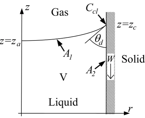
Computations are performed for cases which are axisymmetric or two-dimensional in simple geometries so that calculations may be easily reproduced, thus giving benchmark results for future investigators. In what follows, we consider a meniscus rising against gravity through a cylindrical capillary of radius R. The computational domain is a region in the (r, z)-plane, and the free surface is parameterized by arclength
Figure 2: Illustration showing the computational domain for flow through a capillary with the bulk domainV, liquid-gas free surfaceA1, liquid-solid surfaceA2and contact lineCclall indicated.
of our code as the mesh is refined and to compare our computations to the asymptotic results summarized in §2.2. Then, we will examine Problem A from the view point of analyzing the influence of the radius R
of the capillary on the interface formation dynamics. Finally, the unsteady imbibition of a liquid into a capillary will be considered (hereafter Problem B) and the results compared to published experimental data for this type of flow.
In the (r, z)-plane where the solution is computed, in addition to the equations formulated in§2, on the axis of symmetry for both Problem A and B we have the symmetry conditions in the form of impermeability and zero tangential stress
u·n= 0, n·P·t= 0, (r= 0, 0< z < za),
where za is the a-priori unknown apex height. Additionally, at the apex we have the conditions of (a) smoothness of the free-surface shape and (b) the absence of a surface mass source or sink:
n·er= 0, ρs1v
s
1||·er= 0, (r= 0, z=za).
Before doing the calculations we need to consider estimates for the model’s parameters for the two problems to be studied, leaving free the radius of the capillary as a parameter, whose influence will be examined in§5.
4.1. Typical parameter regime
To obtain estimates for our parameters, consider the flow of a water-glycerol mixture through a capillary of radius R at speed U = 0.01 m s−1. At 60% glycerol this gives fluid properties of ρ ≈ 103 kg m−3, µ≈10−2kg m−1s−1andσ≈7×10⁻²N m−1[33]. On the molecular scale, the interface is a layer of finite
thickness`and, as discussed in [33], the generalized Navier equation and Darcy-type equation are analogous to what one would have for the averaged quantities for flow in a channel of width `. Using this analogy, one would haveβ ∼µ/`and α∼`/µ, so that, taking the coefficients of proportionality as unity as a first approximation, and estimatingρs
1e≈0.6 (so thatλ= 2.5), one has from dynamic wetting experiments [33] that the relaxation time scales as τ =τµµ with τµ extracted from the data asτµ ≈7×10⁻⁶ kg−1 m s2. The equilibrium contact angle is taken asθe= 30◦, so that ρs2e= 1.35. Using these estimates, we have the following parameters of what we will regard as the base state. The parameters independent of the length scale are
and those dependent on the length scale are
Re= 10−2(µm)−1R, St= 10−5(µm)−2R2, α¯= 10−1(µm)R−1, β¯= 10(µm)−1R, = 10−2(µm)R−1.
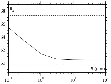
As capillary sizes of interest can range from the millimetre scaleR= 103 µm, relevant, for example, for
applications in microgravity [53], right down to a few tens of nanometresR= 10−2µm [18], the flow can be
dominated by different physical factors. In particular, in large capillaries bulk inertia becomes important as Re > 1 and the surface tension relaxation effect is localized ( 1), being important only close to the contact line, whilst for nanoscale flows inertia becomes negligible (Re 1) and the surface tension relaxation length becomes comparable to the capillary’s width≈1.
Now, we will present benchmark calculations for the steady propagation of a meniscus through a capillary (Problem A) and then consider the time-dependent rise of a meniscus into a capillary (Problem B), which will be compared to experiments.
4.1.1. Problem A: steady propagation of a meniscus through a capillary
For the steady propagation of a meniscus, the ‘base’ of the domain (z= 0) is sufficiently far (quantified below) from the meniscus so that the base can be considered as a ‘far field’. In the far field, the flow is fully developed and the surface variables take their equilibrium values.
The velocity distribution across the capillary base is a Poiseuille profile adapted to allow for slip at the liquid-solid interface that follows from the Navier-slip condition and an additional flux of mass out of the domain via the liquid-solid interface which occurs whenQis non-zero:
u= 0, w=−1 + 1 + ¯q
1/2 + (2 + ¯q)/( ¯β/Ca) 1 + 2/( ¯β/Ca)−r
2
, q¯= 2Qρs2e.
The derivation of this condition is given in the Appendix. Notably, if ¯q= 0 and ¯β/Ca→ ∞, thenw= 1−2r2
which is the usual Poiseuille profile satisfyingdw/dr= 0 atr= 0, w=−1 atr= 1 and R1
r=0w r dr= 0.
Taking the radius of the capillary as R = 100 µm, the parameters dependent on the capillary width becomeRe= 1, St = 10−1, ¯α= 10−3, ¯β = 103 and = 10−4. In this case, = 10−4 is so small that the
distance of the far field is determined by the need for the bulk flow to settle as opposed to for the surface phase to relax to its equilibrium state. It is known that putting the contact line a distance of ten radii away from the ‘far field’ is more than enough for this to be satisfied [54, 27].
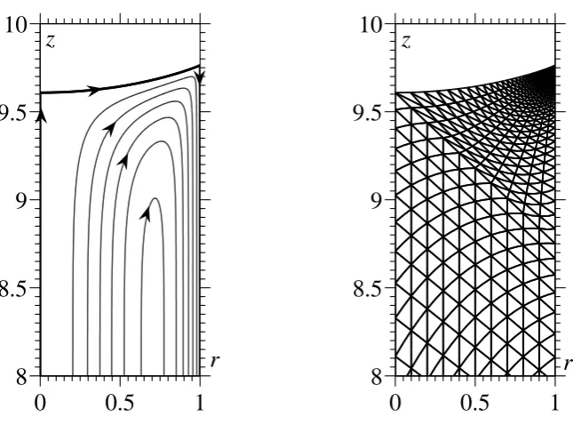
The streamlines for this flow are shown in Figure 3. It can be seen that the motion of the solid with respect to the meniscus drags fluid away from the contact line and that this in turn leads to a flux of fluid into the contact-line zone from the region near the free surface. In Figure 4, one can see that, as predicted by experiments, the motion of the liquid in the vicinity of the contact-line is ‘rolling’, with the liquid-solid interface formed by adsorbing fluid from the bulk. The Poiseuille profile, indicated by parallel streamlines in Figure 3, is established relatively quickly, so that the truncated far field is certainly far enough away from the contact-line region to not influence the results. The mesh is graded, with small elements near the contact line and larger ones further away, so that the essential physics of wetting, occurring on a smaller length scale than the bulk flow, is fully resolved whilst the problem remains computationally tractable. The details of the construction of this mesh are given in [27], where it is shown how the bipolar coordinate system can be utilized to provide circular spines near the contact line and straight ones further away to match with the domain’s shape.
4.1.2. Mesh independence tests
0
0.5
1
8
8.5
9
9.5
10
z
r
0
0.5
1
8
8.5
9
9.5
10
z
[image:18.595.136.459.150.389.2]r
Figure 3: Left: streamlines for the base state simulation in increments of 0.02. Right: corresponding finite element mesh in this region.
−1 −0.8 −0.6 −0.4 −0.2 0
−1 −0.8 −0.6 −0.4 −0.2 0
ε−1
Ca−1(r−1)
ε−1
Ca−1(z−z c)
−1 −0.8 −0.6 −0.4 −0.2 0
−1 −0.8 −0.6 −0.4 −0.2 0
ε−1
Ca−1(r−1)
ε−1
Ca−1(z−z c)
Figure 4: Left: a magnified view of the flow near the contact line for the base state simulation showing the adsorption of the fluid into the liquid-solid interface. The length scale isCa= 10−6and streamlines are in increments of 2.5×10⁻³Ca. Right:
[image:18.595.81.516.490.658.2]0 0.2 0.4 0.6 0.8 1 9.6
9.65 9.7 9.75
1
2 3
4 5 z
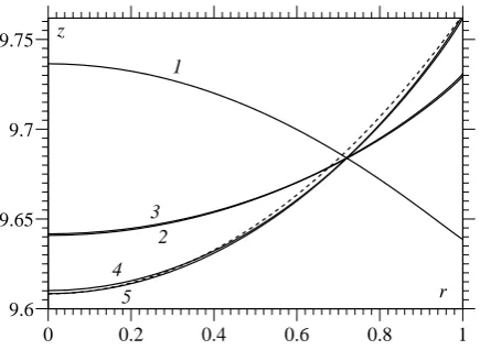
[image:19.595.186.404.115.274.2]r
Figure 5: Convergence of the free-surface shape with curves corresponding to smallest element sizes of 1: 6×10⁻³, 2: 3×10⁻⁴, 3: 2×10⁻⁵, 4: 9×10⁻⁷, 5: 5×10⁻⁸. The dashed line shows the spherical cap approximation which meets the solid at contact
angleθapp= 72.4◦.
In [27], it was shown that the dynamic contact angle θd imposed into the weak formulation can differ from the computed one θc, i.e. the one obtained from the computed free-surface shape, if the mesh is under resolved near the contact line. Rather than imposing the angle in the strong form, and moving the errors to other less observable parts of the numerical scheme, as has often been the case in previous works, it was demonstrated that the difference |θd−θc| provides a simple error-indicator for the scheme. When considering the conventional model, it was shown6 that to resolve both the dynamics of slip and the
free-surface shape near the contact line, so that for the computed angle one has, say,|θd−θc|<0.1◦, the smallest element size lmin must satisfy lmin ≤β¯−1min(5×10⁻², Ca). Then, for the flow considered, this imposes
lmin≤10−3min(5×10−2,10−2) = 10−5. In addition, we now have length scales associated with the physics of interface formation; in particular, the asymptotics forCa, 1 shows that, in the cases considered, the inner most region is on the scaleO(Ca) = 10−6.
To study convergence, it is convenient to consider the following two angles:
θd: The dynamic contact angle featuring in the problem statement; this angle is imposed into the code through the weak formulation, but in the mathematical problem it is a variable whose converged value is to be found.
θc: The angle which the free surface computed for a given spatial resolution of the mesh makes with the solid.
Consider 13 meshes with smallest elements ranging over five orders of magnitude fromlmin= 5×10⁻³ down to lmin = 5×10⁻⁸. Coarser meshes were unable to provide a solution as the computed angle θc increased past 180◦, despite the imposed angleθd being less than 60◦, in the same way as observed in [27]. The change in the free-surface shape during the mesh refinement procedure is shown in Figure 5, where one can see just how bad the approximation is on our most coarse mesh, represented by curve 1. It can be seen that convergence appears to take place in two stages, so that decreasing the smallest element from 3×10⁻⁴
(curve 2) to 2×10⁻⁵ (curve 3) has little influence on the free-surface shape, but, for the reason explained
below, these shapes are yet far from the converged free-surface shape (curve 5) which is obtained only when the mesh elements decrease much further.
The two-stage convergence can be explained by examining the aforementioned angles as the mesh is refined, as shown in Figure 6. One can see that at around lmin = 10−5 the computed angle θc becomes
6Note that in this previous publication the non-dimensionalization is slightly different with ¯β =βL/µ whereas here it is
¯
10−7 10−6 10−5 10−4 10−3 50
60 70 80 90
100 θ
l min
θd θc θa
10−7 10−6 10−5 10−4 10−3
10−3 10−2 10−1 100 101
y=|θ d − θc|
y=|θ a − Θa|
y=|θ d − Θd|
[image:20.595.67.513.115.275.2]l min y
Figure 6: Convergence of the dynamic, computed and apparent angles as the mesh, with smallest element sizelmin, is refined
for the base state simulation. The converged values ofθdandθaare Θd= 60.5◦and Θa= 72.3◦, respectively.
indistinguishable from the dynamic angleθdthat goes into the weak formulation, but at this stageθd, which is a part of the solution, is yet to converge to its final value. This corresponds to curves 2 and 3 in Figure 5. More specifically, we see that|θd−θc|<0.1◦ atlmin = 7×10⁻⁶, close to 10−6 predicted from [27], i.e. the mesh is already sufficiently resolved for the computed angleθc to be close to the angle θd that features in the mathematics of the problem and goes into the weak formulation. However, in our problem, the angleθd is itself a variable and the deviation ofθd from its final value Θd= 60.5◦ is still large|θd−Θd|= 3.8◦. The convergence towards a final solution is then dominated by the requirement to resolve the interface formation dynamics. We have |θd−Θd|<0.1◦ at lmin= 4×10⁻⁷ which again falls close to our estimate and shows the need to resolve the length scaleCa= 10−6. This suggests a new estimate which builds upon that given in [27], that for errors in the angle of the order of 0.1◦, we require
lmin ≤min(5×10⁻²β¯−1, Caβ¯−1,10−1Ca), (49)
which, respectively, ensure that the code resolves the free surface near the contact line (particularly at high
Ca), the length scale on which slip occurs and the dynamics of interface formation.
A frequently used way of simplifying the problem of modelling the flow through a capillary and of easily interpreting theoretical and experimental results for this flow is to approximate the free-surface shape as a spherical cap [55, 56]. Then, the free-surface shape is fully specified by the difference between the contact-line height and apex heighth=zc−za. Usually, the spherical-cap approximation is characterized by the so-called ‘apparent’ contact angleθa, which is the angle that a spherical cap fitted through the apex and the contact line makes with the solid:
θa=π−arccos
− 2h
1 +h2
. (50)
A spherical cap is the free-surface shape obtained in the limit ofCa→0 and by computing θa we will also have a measure of the deviation from this shape due to viscous bending of the free surface.
10−4 10−3 10−2 10−1 100 101 102 103 0.58
0.59 0.6 0.61 0.62
ρs 1
s/ε 2
3 1
10−4 10−3 10−2 10−1 100 101 102 103 −0.8
−0.6 −0.4 −0.2 0
s/ε 1
2
3 u
1t
vs 1t
3
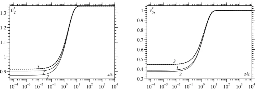
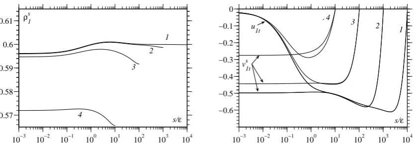
[image:21.595.88.505.117.259.2]2 1
Figure 7: Distribution of the surface variables along the free surface against the scaled distance from the contact lines/. Curves are for (Ca, ) = 1 : (5×10−2,5×10−4), 2 : (10−3,2.5×10−2), 3 : (10−3,5×10⁻⁴). Left: ρs
1 compared to its
asymptotic (equilibrium) value (dashed line). Right: surface velocity tangential to the free surface and bulk velocity tangential to the surface compared to far-field free-surface velocityuf=−0.68 (dashed line).
4.1.3. Convergence to the asymptotic solution as→0,Ca→0
Having established that our computed solution converges under mesh refinement, we now check that this solution converges to the asymptotic results outlined in§2.2 as, Ca→0. As in the the asymptotics, the parameterV2=β/¯ (λ(1 + 4 ¯αβ¯)) is regarded finite in the asymptotic limit considered. To check convergence to the asymptotics, the parameters used in§4.1.2 will remain unchanged except that we now varyandCa
and, for a start, fixV2= 0.1 so that ¯β= ¯α−1= 1.25−1.
Three data sets are considered, with (Ca, ) = 1 : (5×10−2,5×10−4), 2 : (10−3,2.5×10−2), 3 :
(10−3,5×10⁻⁴), so that we can ascertain the influence of decreasing either or Ca by a factor of 50.
The simplest ‘integral’ measure of convergence is the dynamic contact angle whose asymptotic value for this set of parameters is 102.1◦. The obtained solutions for θd for 1−3 are 104.1◦, 107.7◦ and 102◦ so that the deviations from the asymptotic result are 2◦, 5.6◦ and 0.1◦, respectively. Therefore, we have the convergence of the numerically obtained dynamic contact angle to the asymptotic one, with an indication how this convergence is controlled byandCa.
To examine the issue of convergence in more detail, consider the distributions of the surface parameters and the bulk velocity along the interfaces. Deviations of the surface density on the free surfaceρs
1 from its
equilibrium valueρs
1eand the distributions of the tangential components of the surface velocityv1stand the bulk velocity tangential to the free surfaceu1tare shown in Figure 7. As one can see, the magnitude of the variation inρs1 along the free surface is governed byCa, but it isthat determines how far the ‘level’ ofρs1
is from its equilibrium value. As→0,Ca→0, we have thatρs1→ρs1e.
In agreement with the asymptotic results, the surface velocityv1stcoincides withu1tin the intermediate region and the two velocities begin to deviate from each other at around s/ ≈ Ca, i.e. in the inner region, where, as expected, vs
1t remains constant whereas u1t decreases as the contact line is approached. This pattern is clearly seen for data set 3, where both the surface and bulk velocity attain the value of
uf =−0.68 in the outer region, s/ 1, then, as the intermediate asymptotic region is entered, v1st and
u1t remain at this level through this regionCas/1, and as the inner region is reached, the surface velocityvs
1tremains constant up to the contact line, whereasu1tvaries. Sinceρs1is also constant through the
inner region, it is the surface mass flux of the intermediate region that goes into the contact line and hence determine the mass flux that feeds the liquid-solid interface. Notably, as one could already see in Figure 4, forQ6= 0 the contact line is not a stagnation point for the bulk flow, so thatu1t6= 0 at the contact line.