Learning Word Representations from Scarce and Noisy Data with
Embedding Sub-spaces
Ramon F. Astudillo, Silvio Amir, Wang Lin, M´ario Silva, Isabel Trancoso Instituto de Engenharia de Sistemas e Computadores Investigac¸˜ao e Desenvolvimento (INESC-ID)
Rua Alves Redol 9 Lisbon, Portugal
{ramon.astudillo, samir, wlin, mjs, isabel.trancoso}@inesc-id.pt
Abstract
We investigate a technique to adapt unsu-pervised word embeddings to specific ap-plications, when only small and noisy la-beled datasets are available. Current meth-ods use pre-trained embeddings to initial-ize model parameters, and then use the la-beled data to tailor them for the intended task. However, this approach is prone to overfitting when the training is performed with scarce and noisy data. To overcome this issue, we use the supervised data to find an embedding subspace that fits the task complexity. All the word representa-tions are adapted through a projection into this task-specific subspace, even if they do not occur on the labeled dataset. This ap-proach was recently used in the SemEval 2015 Twitter sentiment analysis challenge, attaining state-of-the-art results. Here we show results improving those of the chal-lenge, as well as additional experiments in a Twitter Part-Of-Speech tagging task.
1 Introduction
The success of supervised systems largely depends on the amount and quality of the available train-ing data, oftentimes, even more than the particu-lar choice of learning algorithm (Banko and Brill, 2001). Labeled data is, however, expensive to ob-tain, while unlabeled data is widely available. In order to exploit this fact, semi-supervised learn-ing methods can be used. In particular, it is pos-sible to derive word representations by exploiting word co-occurrence patterns in large samples of unlabeled text. Based on this idea, several meth-ods have been recently proposed to efficiently es-timate word embeddings from raw text, leverag-ing neural language models (Huang et al., 2012; Mikolov et al., 2013; Pennington et al., 2014; Ling
et al., 2015). These models work by maximizing the probability that words within a given window size are predicted correctly. The resulting embed-dings are low-dimensional dense vectors that en-code syntactic and semantic properties of words. Using these word representations, Turian et al. (2010) were able to improve near state-of-the-art systems for several tasks, by simply plugging in the learned word representations as additional fea-tures. However, because these features are esti-mated by minimizing the prediction errors made on a generic, unsupervised, task they might be suboptimal for the intended purposes.
Ideally, word features should be adapted to the specific supervised task. One of the reasons for the success of deep learning models for language problems, is the use unsupervised word embed-dings to initialize the word projection layer. Then, during training, the errors made in the predictions are backpropagated to update the embeddings, so that they better predict the supervised signal (Col-lobert et al., 2011; dos Santos and Gatti, 2014a). However, this strategy faces an additional chal-lenge in noisy domains, such as social media. The lexical variation caused by the typos, use of slang and abbreviations leads to a great number of singletons and out-of-vocabulary words. For these words, the embeddings will be poorly re-estimated. Even worse, words not present on the training set will never get their embeddings up-dated.
In this paper, we describe a strategy to adapt un-supervised word embeddings when dealing with small and noisy labeled datasets. The intuition be-hind our approach is the following. For a given task, only a subset of all the latent aspects captured by the word embeddings will be useful. Therefore, instead of updating the embeddings directly with the available labeled data, we estimate a projec-tion of these embeddings into a low dimensional sub-space. This simple method brings two
mental advantages. On the one hand, we obtain low dimensional embeddings fitting the complex-ity of the target task. On the other hand, we are able to learn new representations for all the words, even if they do not occur in the labeled dataset.
To estimate the low dimensional sub-space, we propose a simple non-linear model equivalent to a neural network with one single hidden layer. The model is trained in supervised fashion on the la-beled dataset, learning jointly the sub-space pro-jection and a classifier for the target task. Using this model, we built a system to participate in the SemEval 2015 Twitter sentiment analysis bench-mark (Rosenthal et al., 2015). Our submission at-tained state-of-the-art results without hand-coded features or linguistic resources (Astudillo et al., 2015). Here, we further investigate this approach and compare it against several state-of-the-art sys-tems for Twitter sentiment classification. We also report on additional experiments to assess the ad-equacy of this strategy in other natural language problems. To this end, we apply the embedding sub-space layer to Ling et al. (2015) deep learning model for part-of-speech tagging. Even though the gains were not as significant as in the senti-ment polarity prediction task, the results suggest that our method is indeed generalizable to other problems.
The rest of the paper is organized as follows: the related work is reviewed in Section 2. Section 3, briefly describes the model used to pre-train the word embeddings. In Section 4, we introduce the concept of embedding sub-space, as well as the the non-linear sub-space model for text classifica-tion. Section 5, details the experiments performed with the SemEval corpora. Section 6 describes ad-ditional experiments applying the embedding sub-space method to a Part-of-Speech tagging model for Twitter data. Finally, Section 7 draws the con-clusions.
2 Related Work
NLP systems can benefit from a very large pool of unlabeled data. While raw documents are usu-ally not annotated, they contain structure, which can be leveraged to learn word features. Con-text is one strong indicator for word similarity, as related words tend to occur in similar con-texts (Firth, 1968). Approaches that are based on this concept include, Latent Semantic Analysis, where words are represented as rows in the
low-rank approximation of a term co-occurrence ma-trix (Dumais et al., 1988), word clusters obtained with hierarchical clustering algorithms based on Hidden Markov Models (Brown et al., 1992), and continuous word vectors learned with neural lan-guage models (Bengio et al., 2003). The result-ing clusters and vectors, can then be used as more generalizable features in supervised tasks, as they also provide representations for words not present in the labeled data (Bespalov et al., 2011; Owoputi et al., 2013; Chen and Manning, 2014).
A great amount of work has been done on the problem of learning better word representations from unsupervised data. However, not many stud-ies have discussed the best ways to use them in supervised tasks. Typically, in these cases, word representations are directly used as features or to initialize the parameters of more complex mod-els. In some tasks, this approach is however prone to overfitting. The work presented here aims to provide a simple approach to overcome this last scenario. It is thus directly related to Labutov and Lipson (2013), where a method to learn task-specific representations from general pre-trained embeddings was presented. In this work, new fea-tures were estimated with a convex objective func-tion that combined the log-likelihood of the train-ing data, with regularization penaliztrain-ing the Frobe-nius norm of the distortion matrix. That is, the ma-trix of the differences between the original and the new embeddings. Even though the adapted em-beddings performed better than the purely unsu-pervised features, both were significantly outper-formed by a simple bag-of-words baseline.
were estimated with a neural network that mini-mized a linear combination of two loss functions, one penalized the errors made at predicting the center word within a sequence of words, while the other penalized mistakes made at deciding the sen-timent label. Weakly labeled data has also been used to refine unsupervised embeddings, by re-training them to predict the noisy labels before us-ing the actual task-specific supervised data (Sev-eryn and Moschitti, 2015).
3 Unsupervised Structured Skip-Gram Word Embeddings
Word embeddings are generally trained by opti-mizing an objective function that can be measured without annotations. One popular approach is to estimate the embeddings by maximizing the prob-ability that the words within a given window size are predicted correctly. Our previous work has compared several such models, namely the skip-gram and CBOW architectures (Mikolov et al., 2013), GloVe (Pennington et al., 2014), and the structured skip-gram approach (Ling et al., 2015), suggesting that they all have comparable capabil-ities. Thus, in this study we only use embeddings derived with the structured skip-gram approach, a modification of the skip-gram architecture that has been shown to outperform the original model in syntax based tasks such as, part-of-speech tagging and dependency parsing.
Central to the structured skip-gram is a log lin-ear model of word prediction. Letw = idenote that a word at a given position of a sentence is the i-th word on a vocabulary of size v, and let
wp = j denote that the wordp positions further
in the sentence is the j-th word on the vocabu-lary. The structured skip-gram models the follow-ing probability:
p(wp=j|w=i)∝expCpj·E·wi (1)
Here, wi ∈ {1,0}v×1 is a one-hot representa-tion of w = i. That is, a vector of zeros of the size of the vocabularyvwith a 1 on thei-th entry of the vector. The symbol·denotes internal prod-uct andexp() acts element-wise. The log-linear model is parametrized by the following matrices: E ∈ Re×v, is the embedding matrix,
transform-ing the one-hot representation into a compact real valued space of sizee,Cpj ∈Rv×e is a set of
out-put matrices, one for each relative word positionp,
projecting the real-valued representation to a vec-tor with the size of the vocabulary v. By learn-ing a different matrix Cp for each relative word
position, the model captures word order informa-tion, unlike the original skip-gram approach that uses only one output matrix. Finally, a distribution over all possible words is attained by exponentiat-ing and normalizexponentiat-ing over thevpossible options. In practice, negative sampling is used to avoid having to normalize over the whole vocabulary (Goldberg and Levy, 2014).
As most other neural network models, the struc-tured skip-gram is trained with gradient-based methods. After a model has been trained, the low dimensional embeddingE·wi ∈ Re×1
encapsu-lates the information about each wordwi and its
surrounding contexts. This embbeding can thus be used as input to other learning algorithms to further enhance performance.
4 Adapting Embeddings with Sub-space Projections
As detailed in the introduction and related work, word embeddings are a useful unsupervised tech-nique to attain initial model values or features prior to supervised training. These models can be then retrained using the available labeled data. However, even if the embeddings provide a com-pact real valued representation of each word in a vocabulary, the total number of parameters in the model can be rather high. If, as it is often the case, only a small amount of supervised data is available, this can lead to severe overfitting. Even if regularization is used to reduce the overfitting risk, only a reduced subset of the words will actu-ally be present in the labeled dataset. Words not seen during training will never get their embed-dings updated. Furthermore, rare words will re-ceive very few updates, and thus their embeddings will be poorly adapted for the intended task. We propose a simple solution to avoid this problem.
4.1 Embedding Sub-space
Let E ∈ Re×v denote the original embedding
matrix obtained, e.g. with the structured skip-gram model described in Equation 1. We define the adapted embedding matrix as the factorization S·E, whereS∈Rs×e, withse. We estimate
matrixEinto a sub-space of dimensions.
The idea of embedding sub-space rests on two fundamental principles:
1. With dimensionality reduction of the embed-dings, the model can better fit the complexity of the task at hand or the amount of available data.
2. Using a projection, all the embeddings are indirectly updated, not only those of words present in the labeled dataset.
One question that arises from this approach, is if the estimated projection is also optimal for the words not present in the labeled dataset. We as-sume that the words on the labeled dataset are, to some extent, representative of the words found in the unlabeled corpus. This is a reasonable assump-tion since both datasets can be seen as samples drawn from the same power-law distribution. If this holds, for everyunknownword, there will be some other word sufficiently close it in the embed-ding space. Consequently, the projection matrix S will also be approximately valid for those un-seen words. It is often the case that a relatively small number of words of the labeled dataset are not present on the unlabeled corpus. These words are not represented inE. One way to deal with this case, is to simply set the embeddings of unknown words to zero. But in this case, the embeddings will not be adapted during training. Random ini-tializations of the embeddings seems to be help-ful for tasks that have a higher penalty for missing words, although it remains unclear if better initial-ization strategies exist.
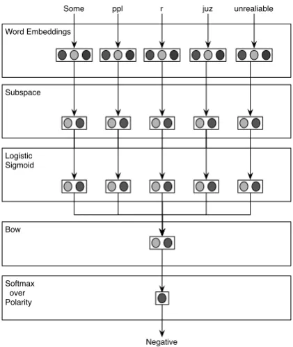
4.2 Non-Linear Embedding Sub-space Model The concept of embedding sub-space can be ap-plied to log-linear classifiers or any deep learning architecture that uses embeddings. We now de-scribe an application of this method for short text classification tasks. In what follows, we will refer to this approach as Non-Linear Sub-space Embed-ding (NLSE) model. The NLSE can be interpreted as a simple feed-forward neural network model (Rumelhart et al., 1985) with one single hidden layer utilizing the embedding sub-space approach, as depicted in Fig. 1. Let
m= [w1· · ·wn] (2)
denote a message of n words. Each column w∈ {0,1}v×1 of m represents a word in one-hot form, as described in Section 3. Let y de-note a categorical random variable overKclasses. The NLSE model, estimates thus the probability of each possible categoryy = k ∈ K given a mes-sagemas
p(y =k|m)∝exp (Yk·h·1). (3)
Here,h∈ {0,1}e×nare the activations of the
hid-den layer for each word, given by
h=σ(S·E·m) (4) whereσ()is a sigmoid function acting on each element of the matrix. The matrix Y ∈ R3×s
maps the embedding sub-space to the classifica-tion space and1 ∈ 1n×1 is a matrix of ones that sums the scores for all words together, prior to nor-malization. This is equivalent to a bag-of-words assumption. Finally, the model computes a prob-ability distribution over the K classes, using the softmaxfunction.
Compared to a conventional feed-forward net-work employing embeddings for natural language classification tasks, two main differences arise. First, the input layer is factorized into two com-ponents, the embeddings attained in unsupervised form,E, and the projection matrixS. Second, the size of the sub-space, in which the embeddings are projected, is much smaller than that of the origi-nal embeddings with typical reductions above one order of magnitude. As usual in this kind of mod-els, all the parameters can be trained with gradient methods, using the backpropagation update rule.
Softmax over Polarity Subspace Word Embeddings
ppl r juz unrealiable Some
Bow
Negative Logistic
[image:5.595.76.287.65.315.2]Sigmoid
Figure 1: Illustration of the NLSE model, applied to sentiment polarity prediction.
Positive Neutral Negative Development 3230 4109 1265
Tweets 2015 1032 983 364
Tweets 2014 982 669 202
Tweets 2013 1572 1640 601
Table 1: Number of examples per class in each SemEval dataset. The first row shows the training data; the other rows are sets used for testing.
need to be enriched with additional hand-crafted features that try to capture more discriminative as-pects of the content, most of which require exter-nal tools (e.g., part-of-speech taggers and parsers) or linguistic resources (e.g., dictionaries and sen-timent lexicons) (Miura et al., 2014; Kiritchenko et al., 2014). With the embedding sub-space ap-proach, however, we are able to attain state-of-the-art performance while requiring only minimal processing of the data and few hyperparameters. To make our results comparable to other systems for this task, we adopted the guidelines from the benchmark. Our system was trained and tuned using only the development data. The evaluation was performed on the test sets, shown in Table 1, and we report the results in terms of the average F-measure for the positive and negative classes.
5.1 Experimental Setup
The first step of our approach requires a corpus of raw text for the unsupervised pre-training of the embedding matrixE. We resorted to the corpus of 52 million tweets used in (Owoputi et al., 2013) and the tokenizer described in the same work. The messages were previously pre-processed as fol-lows: lower-casing, replacing Twitter user men-tions and URLs with special tokens and reducing any character repetition to at most 3 characters. Words occurring less than 40 times in the cor-pus were discarded, resulting in a vocabulary of around 210,000 types. Then, a modified version of theword2vectool1 was used to compute the
word embeddings, as described in Section 3. The window size and negative sampling rate were set to 5 and 25 words, respectively, and embeddings of 50, 200, 400 and 600 dimensions were built.
Our system accepts as input a sentence rep-resented as a matrix, obtained by concatenating theone-hotvectors that represent each individual word. Therefore, we first performed the afore-mentioned normalization and tokenization steps and then, converted each tweet into this represen-tation. The development set was split into 80%
for parameter learning and20%for model evalu-ation and selection, maintaining the original rela-tive class proportions in each set. All the weights were initialized uniformly at random, as proposed in (Glorot and Bengio, 2010). The model was trained with conventional Stochastic Gradient De-scent (Rumelhart et al., 1985) with a fixed learning rate of 0.01, and the weights were updated after each message was processed. Variations of learn-ing rate to smaller values, e.g. 0.005, were con-sidered but did not lead to a clear pattern. We ex-plored different configurations of the hyperparam-eters e (embedding size) and s (sub-space size). Model selection was done by early stopping, i.e., we kept the configuration with best F-measure on the evaluation set after5-8iterations.
5.2 Results
In general, the NLSE model showed consistent and fast convergence towards the optimum in very few iterations. Despite using class log-likelihood as training criterion, it showed good performance in terms of the average F-measure for positive and negative sentiments. We found that all em-bedding sizes yield comparable performances,
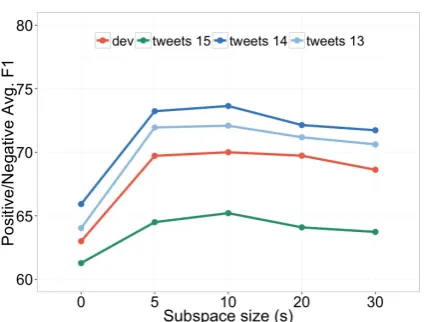
Figure 2: Average F-measure on the SemEval test sets varying with embedding sub-space size s. Sub-space size 0 used to denote the baseline (log-linear model).
though larger embeddings tend to perform better. Therefore, we only report results obtained with the 600 dimensional vectors. In Figure 2, we show the variation of system performance with sub-space size s. The baseline is a log-linear using the em-beddings inE as features. As it can be seen, the performance is sharply improved when the em-bedding sub-spaces are used. By choosing dif-ferent values ofs, we can adjust the model to the complexity of the task and the amount of labeled data available. Given the small size of the train-ing set, the best results were attained with the use of smaller sub-spaces, in the range of5-10 dimen-sions.
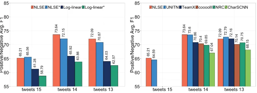
Figure 3, presents the main results of the ex-perimental evaluation. As baselines, we consid-ered two simple approaches:LOG-LINEAR, which uses the unsupervised embeddings directly as fea-tures in a log-linear classifier, andLOG-LINEAR*, also using the unsupervised embeddings as fea-tures in a log-linear classifier, but updating the em-beddings with the training data. These baselines, were compared against two variations of the non-linear sub-space embedding model: NLSE, where we only train theSandYweights while the em-beddings are kept fixed, and NLSE*, where we also update the embedding matrix during training. For these experiments, we set s = 10. The re-sults in Figure 3a, show that our model largely outperforms the simpler baselines. Furthermore, we observe that updating the embeddings always leads to inferior results. This suggests that
pre-computed embeddings should be kept fixed, when little labeled data is available to re-train them. Comparison with the state-of-the-art
We now compare the NLSE model with state-of-the-art systems, including the best submissions to previous SemEval benchmarks. We also include two other approaches that are related to the one here proposed, where a neural network initialized with pre-trained word embeddings is used to learn relevant features. Specifically, we compare the following systems:
• NRC (Kiritchenko et al., 2014), a support vector machine classifier with a large set of hand-crafted features, including word and character n-grams, brown clusters, POS tags, morphological features, and a set of features based on five sentiment lexicons. Most of the performance was due to the combination of these lexicons. This was the top system in the 2013 edition of SemEval.
• TEAMX (Miura et al., 2014), a logistic re-gression classifier using a similar set of fea-tures. Additional features based on two dif-ferent POS taggers and a word sense dis-ambiguator were also included in the model. This approach attained the highest ranking in the 2014 edition.
• CHARSCNN (dos Santos and Gatti, 2014b), a deep learning architecture with two con-volutional layers that exploit character-level and word-level information. The features are extracted by converting a sentence into a se-quence of word embeddings, and the individ-ual words into sequences of character embed-dings. Convolution filters followed bymax
pooling are applied to these sequences, to produce fixed size vectors. These vectors are then combined and transfered to a set of non-linear activation functions, to generate more complex representations of the input. The predictions, based on these learned features are computed with asoftmaxclassifier.
[image:6.595.75.288.62.223.2](a) Comparison of two baselines with two variations
[image:7.595.77.522.63.225.2]of the NLSE model (b) Performance of state-of-the-art systems for Twitter senti-ment prediction Figure 3: Average F-measure on the SemEval test sets
averagepooling. The final feature vector is
obtained by concatenating these representa-tions and Kiritchenko et al. (2014) feature set.
• UNITN (Severyn and Moschitti, 2015), an-other deep convolutional neural network that jointly learns internal representations and a
softmaxclassifier. The network is trained
in three steps: (i) unsupervised pre-training of embeddings, (ii) refinement of the em-beddings using a weakly labeled corpus, and (iii) fine tuning the model with the labeled data from SemEval. It should be noted that the system was trained with a labeled corpus 65% larger than ours2. This system made the
best submission on the 2015 edition of the benchmark.
The results in Figure 3b, show that despite be-ing simpler and requirbe-ing less resources and la-beled data, the NLSE model is extremely compet-itive, even outperforming most other systems, in predicting the sentiment polarity of Twitter mes-sages.
6 Generalization to Other Tasks
While the embedding sub-space method works well for the sentiment prediction task, we would like to know its impact in other settings that are known to benefit from unsupervised embeddings. Thus, we decided to replicate the part-of-speech tagging work in (Ling et al., 2015), where pre-training embeddings have been shown to improve
2The UNITN system was trained with around 11,400
la-beled examples, whereas we used only 6,900.
the quality of the results significantly. 6.1 Sub-space Window Model
Part-of-speech tagging is a word labeling task, where each word is to be labeled with its syntactic function in the sentence. More formally, given an input sentencew1, . . . , wnofnwords, we wish to predict a sequence of labelsy1, . . . , yn, which are
the POS tags of each of the words. This task is scored by the ratio between the number of correct labels and the number of words to be labeled.
We modified (Collobert et al., 2011) window model, to include the sub-space matrix S. The probability of labeling the wordwtwith the POS
tagkis given by
p(y=k|mtt+−pp)∝exp (Yk·ht+b), (5)
where
mtt+−pp = [wt−p· · ·wt· · ·wt+p] (6)
denotes a context window of words around the
t-th word, with a total span of2p+ 1 words. ht
denotes the activations of a hidden layer given by
ht= tanh
H·
S·E·wt+p
· · ·
S·E·wt
· · ·
S·E·wt−p
. (7)
sub-spaceS matrices, the model is parametrized by the weightsH∈Rh×psandY∈Rv×has well
as a biasb∈Rv×1.
Note that ifS is set to the identity matrix, this would be equivalent to the original Collobert et al. (2011) model.
Tanh
Softmax over Tags Subspace Word Embeddings
ppl r juz unrealiable Some
Window
Verb
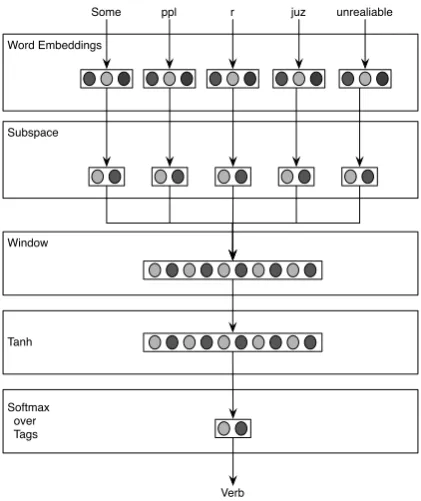
Figure 4: Illustration of the window model by (Collobert et al., 2011) using a sub-space layer.
6.2 Experiments
Tests were performed in Gimpel et al. (2011) Twit-ter POS dataset, which uses the universal POS tag set composed by 25 different labels (Petrov et al., 2012). The dataset contains 1000 annotated tweets for training, 327 tweets for tuning and 500 tweets for testing. The number of word tokens in these sets are 15000, 5000 and 7000, respectively. There are 5000, 2000 and 3000 word types.
Once again, we initialized the embeddings with unsupervised pre-training using the struc-tured skip-gram approach. As for the hyperpa-rameters of the model, we used embeddings with
e= 50dimensions, a hidden layer withh = 200
dimensions and a context ofp= 2as used in (Ling et al., 2015). Training employed mini-batch gradi-ent descgradi-ent, with mini batches of 100 sentences and a momentum of0.95. The learning rate was set to 0.2. Finally, we used early stopping by choosing the epoch with the highest accuracy in
the tuning set. As for the sub-space layer size, we tried three different hyperparameterizations: 10,
30and50dimensions.
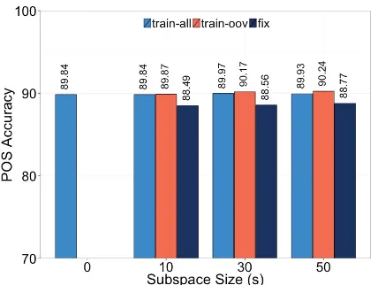
[image:8.595.76.287.159.410.2]6.3 Results
Figure 5 displays the results. Using the setup that led to the best results in the sentiment prediction task (FIX), that is, fixingE and updatingS, leads to lower accuracies than the baseline (TRAIN-ALL,
s= 0). We also see that different values ofsdo not have a very strong impact in the final results.
Sentiment polarity prediction and POS tagging differ in multiple aspects and there may be more than one reason for this poorer performance. One particularly relevant aspect, in our opinion, is the way words that have no pre-trained embedding are treated. In the case of sentiment prediction, these words were set to having and embedding of zero. This fits the use of the bag-of-words assumption and the fact that only one label is produced per message, as there are many other words to draw evidence from. In the case of POS tagging a hy-pothesis must be drawn for each word, using a shorter context. Thus, ignoring a word means that context is used instead, which is a frequent cause of errors.
One way around this problem would be to up-date the parameters ofS andE, but this leads to results similar to the experiment without the sub-space projections (TRAIN-ALL). This is expected as the sub-space layer was designed to work on fixed word embeddings, if these are updated its benefits are lost. Thus, we solve this problem by fixing all the embeddings, except for the word types not found in the pre-training corpus. That is, instead of leaving the unknown words as the zero vector, we use the labeled data to learn a bet-ter representation. Using this setup (TRAIN-OOV), we can obtain a small but consistent improvement over the baseline. While these improvements are not significant, as this task is not as prone to over-fitting as in sentiment analysis, this is a good check of the validity of our method.
7 Conclusions
Figure 5: Results for the part-of-speech task on the ARK POS dataset, for different strategies to update the embeddings and with variations of the sub-space size. Sub-space size 0 used to denote the baseline (window model).
hand, it reduces the number of model parameters to fit the complexity of the task. These properties make this method particularly useful for the cases where only small amounts of noisy data are avail-able to train the model.
Experiments on the SemEval challenge corpora validated these ideas, showing that such a simple approach can attain state-of-the-art results compa-rable with the best systems of past SemEval edi-tions and often outperforming them in all datasets. It should be noted that this is attained while keep-ing the original embeddkeep-ing matrix E fixed and only learning the projectionSwith the supervised data. Additional experiments on the Twitter POS tagging task indicate however that, the technique is not always as effective as in the sentiment clas-sification task. One possible explanation for the different behavior is the use of embeddings of ze-ros for words without pre-trained embedding. It is plausible that this has a stronger effect on the POS tagging task. Another aspect to be taken into ac-count is the fact that both tasks could have a differ-ent complexity which would explain why adapting Ein the POS taks yields better results. Optimality of the embeddings for each of the tasks might also come into play here.
The implementation of the proposed method and our Twitter Sentiment Analysis system has been made publicly available3.
3https://github.com/ramon-astudillo/
NLSE
Acknowledgments
This work was partially supported by Fundac¸˜ao para a Ciˆencia e Tecnologia (FCT), through contracts UID/CEC/50021/2013, EXCL/EEI-ESS/0257/2012 (DataStorm), research project with reference UTAP-EXPL/EEI-ESS/0031/2014, EU project SPEDIAL (FP7 611396), grant number SFRH/BPD/68428/2010 and Ph.D. scholarship SFRH/BD/89020/2012.
References
Ramon F. Astudillo, Silvio Amir, Wang Ling, Bruno Martins, M´ario Silva, and Isabel Trancoso. 2015. Inesc-id: Sentiment analysis without hand-coded features or liguistic resources using embedding
sub-spaces. In Proceedings of the 9th International
Workshop on Semantic Evaluation, SemEval ’2015, Denver, Colorado, June. Association for Computa-tional Linguistics.
Michele Banko and Eric Brill. 2001. Scaling to very very large corpora for natural language
disambigua-tion. In Proceedings of the 39th Annual Meeting
on Association for Computational Linguistics, pages 26–33. Association for Computational Linguistics. Mohit Bansal, Kevin Gimpel, and Karen Livescu.
2014. Tailoring continuous word representations for
dependency parsing. InProceedings of the Annual
Meeting of the Association for Computational Lin-guistics.
Yoshua Bengio, R´ejean Ducharme, Pascal Vincent, and Christian Janvin. 2003. A neural probabilistic
lan-guage model. The Journal of Machine Learning
Re-search, 3:1137–1155.
Dmitriy Bespalov, Bing Bai, Yanjun Qi, and Ali Shok-oufandeh. 2011. Sentiment classification based on supervised latent n-gram analysis. InProceedings of the 20th ACM international conference on Informa-tion and knowledge management, pages 375–382. ACM.
Peter F. Brown, Peter V. deSouza, Robert L. Mer-cer, Vincent J. Della Pietra, and Jenifer C. Lai. 1992. Class-based n-gram models of natural
lan-guage. Comput. Linguist., 18(4):467–479,
Decem-ber.
Danqi Chen and Christopher D Manning. 2014. A fast and accurate dependency parser using neural
net-works. InProceedings of the 2014 Conference on
Empirical Methods in Natural Language Processing (EMNLP), pages 740–750.
Ronan Collobert, Jason Weston, L´eon Bottou, Michael Karlen, Koray Kavukcuoglu, and Pavel Kuksa. 2011. Natural language processing (almost) from
scratch. The Journal of Machine Learning
Cicero dos Santos and Maira Gatti. 2014a. Deep convolutional neural networks for sentiment
analy-sis of short texts. InProceedings of COLING 2014,
the 25th International Conference on Computational Linguistics: Technical Papers, pages 69–78, Dublin, Ireland, August. Dublin City University and Associ-ation for ComputAssoci-ational Linguistics.
Cıcero Nogueira dos Santos and Maıra Gatti. 2014b. Deep convolutional neural networks for sentiment analysis of short texts. InProceedings of the 25th In-ternational Conference on Computational Linguis-tics (COLING), Dublin, Ireland.
Susan T Dumais, George W Furnas, Thomas K Lan-dauer, Scott Deerwester, and Richard Harshman. 1988. Using latent semantic analysis to improve
ac-cess to textual information. In Proceedings of the
SIGCHI conference on Human factors in computing systems, pages 281–285. ACM.
John Rupert Firth. 1968. Selected papers of JR Firth,
1952-59. Indiana University Press.
Kevin Gimpel, Nathan Schneider, Brendan O’Connor, Dipanjan Das, Daniel Mills, Jacob Eisenstein, Michael Heilman, Dani Yogatama, Jeffrey Flanigan, and Noah A. Smith. 2011. Part-of-speech tagging for twitter: annotation, features, and experiments. In
Proceedings of the 49th Annual Meeting of the Asso-ciation for Computational Linguistics: Human Lan-guage Technologies: short papers - Volume 2, HLT ’11, Stroudsburg, PA, USA. Association for Compu-tational Linguistics.
Xavier Glorot and Yoshua Bengio. 2010. Understand-ing the difficulty of trainUnderstand-ing deep feedforward neural networks. In International conference on artificial intelligence and statistics, pages 249–256.
Alec Go, Richa Bhayani, and Lei Huang. 2009. Twit-ter sentiment classification using distant supervision.
CS224N Project Report, Stanford, pages 1–12. Yoav Goldberg and Omer Levy. 2014. word2vec
explained: deriving mikolov et al.’s
negative-sampling word-embedding method. arXiv preprint
arXiv:1402.3722.
Eric H. Huang, Richard Socher, Christopher D. Man-ning, and Andrew Y. Ng. 2012. Improving word representations via global context and multiple word prototypes. InProceedings of the 50th Annual Meet-ing of the Association for Computational LMeet-inguis- Linguis-tics: Long Papers - Volume 1, ACL ’12, pages 873– 882, Stroudsburg, PA, USA. Association for Com-putational Linguistics.
Svetlana Kiritchenko, Xiaodan Zhu, and Saif M Mo-hammad. 2014. Sentiment analysis of short in-formal texts. Journal of Artificial Intelligence Re-search, pages 723–762.
Igor Labutov and Hod Lipson. 2013. Re-embedding words. InProceedings of the 51st annual meeting of the ACL, pages 489–493.
Wang Ling, Chris Dyer, Alan Black, and Isabel Trancoso. 2015. Two/too simple adaptations of
word2vec for syntax problems. In Proceedings of
the 2015 Conference of the North American Chap-ter of the Association for Computational Linguis-tics: Human Language Technologies. Association for Computational Linguistics.
Tomas Mikolov, Ilya Sutskever, Kai Chen, Greg Cor-rado, and Jeffrey Dean. 2013. Distributed represen-tations of words and phrases and their
composition-ality. In27th Annual Conference on Neural
Infor-mation Processing Systems.
Yasuhide Miura, Shigeyuki Sakaki, Keigo Hattori, and Tomoko Ohkuma. 2014. Teamx: A sentiment ana-lyzer with enhanced lexicon mapping and weighting
scheme for unbalanced data. InProceedings of the
8th International Workshop on Semantic Evaluation (SemEval 2014), pages 628–632, Dublin, Ireland, August. Association for Computational Linguistics.
Preslav Nakov, Zornitsa Kozareva, Alan Ritter, Sara Rosenthal, Veselin Stoyanov, and Theresa Wilson. 2013. Semeval-2013 task 2: Sentiment analysis in twitter.
Olutobi Owoputi, Chris Dyer, Kevin Gimpel, Nathan Schneider, and Noah A. Smith. 2013. Improved part-of-speech tagging for online conversational text with word clusters. InIn Proceedings of NAACL.
Jeffrey Pennington, Richard Socher, and Christopher D
Manning. 2014. Glove: Global vectors for
word representation. Proceedings of the Empiricial
Methods in Natural Language Processing (EMNLP 2014), 12.
Slav Petrov, Dipanjan Das, and Ryan McDonald. 2012. A universal part-of-speech tagset. InProceedings of the Eight International Conference on Language Re-sources and Evaluation (LREC’12). European Lan-guage Resources Association (ELRA), may.
Sara Rosenthal, Preslav Nakov, Svetlana Kiritchenko, Saif M Mohammad, Alan Ritter, and Veselin Stoy-anov. 2015. Semeval-2015 task 10: Sentiment
analysis in twitter. In Proceedings of the 9th
In-ternational Workshop on Semantic Evaluation, Se-mEval ’2015, Denver, Colorado, June. Association for Computational Linguistics.
David E Rumelhart, Geoffrey E Hinton, and Ronald J Williams. 1985. Learning internal representations by error propagation. Technical report, DTIC Doc-ument.
Duyu Tang, Furu Wei, Bing Qin, Ting Liu, and Ming Zhou. 2014a. Coooolll: A deep learning system for twitter sentiment classification. SemEval 2014, page 208.
Duyu Tang, Furu Wei, Nan Yang, Ming Zhou, Ting Liu, and Bing Qin. 2014b. Learning sentiment-specific word embedding for twitter sentiment clas-sification. InProceedings of the 52nd Annual Meet-ing of the Association for Computational LMeet-inguis- Linguis-tics, pages 1555–1565.