Graph-based Dependency Parsing with Bidirectional LSTM
Wenhui Wang Baobao Chang
Key Laboratory of Computational Linguistics, Ministry of Education. School of Electronics Engineering and Computer Science, Peking University,
No.5 Yiheyuan Road, Haidian District, Beijing, 100871, China
Collaborative Innovation Center for Language Ability, Xuzhou, 221009, China. {wangwenhui,chbb}@pku.edu.cn
Abstract
In this paper, we propose a neural network model for graph-based dependency pars-ing which utilizes Bidirectional LSTM (BLSTM) to capture richer contextual in-formation instead of using high-order fac-torization, and enable our model to use much fewer features than previous work. In addition, we propose an effective way to learn sentence segment embedding on sentence-level based on an extra forward LSTM network. Although our model uses only first-order factorization, experiments on English Peen Treebank and Chinese Penn Treebank show that our model could be competitive with previous higher-order graph-based dependency parsing models and state-of-the-art models.
1 Introduction
Dependency parsing is a fundamental task for lan-guage processing which has been investigated for decades. It has been applied in a wide range of ap-plications such as information extraction and ma-chine translation. Among a variety of dependency parsing models, graph-based models are attractive for their ability of scoring the parsing decisions on a whole-tree basis. Typical graph-based mod-els factor the dependency tree into subgraphs, in-cluding single arcs (McDonald et al., 2005), sib-ling or grandparent arcs (McDonald and Pereira, 2006; Carreras, 2007) or higher-order substruc-tures (Koo and Collins, 2010; Ma and Zhao, 2012) and then score the whole tree by summing scores of the subgraphs. In these models, subgraphs are usually represented as high-dimensional feature vectors which are then fed into a linear model to learn the feature weights.
However, conventional graph-based models
heavily rely on feature engineering and their per-formance is restricted by the design of features. In addition, standard decoding algorithm (Eisner, 2000) only works for the first-order model which limits the scope of feature selection. To incor-porate high-order features, Eisner algorithm must be somehow extended or modified, which is usu-ally done at high cost in terms of efficiency. The fourth-order graph-based model (Ma and Zhao, 2012), which seems the highest-order model so far to our knowledge, requiresO(n5) time andO(n4)
space. Due to the high computational cost, high-order models are normally restricted to produc-ing only unlabeled parses to avoid extra cost in-troduced by inclusion of arc-labels into the parse trees.
To alleviate the burden of feature engineering, Pei et al. (2015) presented an effective neural net-work model for graph-based dependency parsing. They only use atomic features such as word uni-grams and POS tag uniuni-grams and leave the model to automatically learn the feature combinations. However, their model requires many atomic fea-tures and still relies on high-order factorization strategy to further improve the accuracy.
Different from previous work, we propose an LSTM-based dependency parsing model in this paper and aim to use LSTM network to capture richer contextual information to support parsing decisions, instead of adopting a high-order factor-ization. The main advantages of our model are as follows:
• By introducing Bidirectional LSTM, our model shows strong ability to capture poten-tial long range contextual information and ex-hibits improved accuracy in recovering long distance dependencies. It is different to pre-vious work in which a similar effect is usually achieved by high-order factorization.
over, our model also eliminates the need for setting feature selection windows and re-duces the number of features to a minimum level.
• We propose an LSTM-based sentence seg-ment embedding method named LSTM-Minus, in which distributed representation of sentence segment is learned by using subtrac-tion between LSTM hidden vectors. Experi-ment shows this further enhances our model’s ability to access to sentence-level informa-tion.
• Last but important, our model is a first-order model using standard Eisner algorithm for decoding, the computational cost remains at the lowest level among graph-based models. Our model does not trade-off efficiency for accuracy.
We evaluate our model on the English Penn Treebank and Chinese Penn Treebank, experi-ments show that our model achieves competi-tive parsing accuracy compared with conventional high-order models, however, with a much lower computational cost.
2 Graph-based dependency parsing In dependency parsing, syntactic relationships are represented as directed arcs between head words and their modifier words. Each word in a sen-tence modifies exactly one head, but can have any number of modifiers itself. The whole sentence is rooted at a designated special symbolROOT, thus the dependency graph for a sentence is constrained to be a rooted, directed tree.
For a sentencex, graph-based dependency pars-ing model searches for the highest-scorpars-ing tree of
x:
y∗(x) = arg max ˆ
y∈Y(x) Score(x,yˆ;θ) (1)
Herey∗(x)is the tree with the highest score,Y(x)
is the set of all valid dependency trees for x and
Score(x,yˆ;θ) measures how likely the tree yˆis the correct analysis of the sentence x, θ are the model parameters. However, the size of Y(x)
grows exponentially with respect to the length of the sentence, directly solving equation (1) is im-practical.
[image:2.595.316.521.62.171.2]The common strategy adopted in the graph-based model is to factor the dependency treeyˆinto
Figure 1: First-order, Second-order and Third-order factorization strategy. Herehstands for head word,m stands for modifier word, sandt stand for the sibling ofm. gstands for the grandparent ofm.
a set of subgraph cwhich can be scored in isola-tion, and score the whole treeyˆby summing score of each subgraph:
Score(x,yˆ;θ) =X
c∈yˆ
ScoreC(x, c;θ) (2)
Figure 1 shows several factorization strategies. The order of the factorization is defined accord-ing to the number of dependencies that subgraph contains. The simplest first-order factorization (McDonald et al., 2005) decomposes a depen-dency tree into single dependepen-dency arcs. Based on the first-order factorization, second-order fac-torization (McDonald and Pereira, 2006; Carreras, 2007) brings sibling and grandparent information into their model. Third-order factorization (Koo and Collins, 2010) further incorporates richer con-textual information by utilizing grand-sibling and tri-sibling parts.
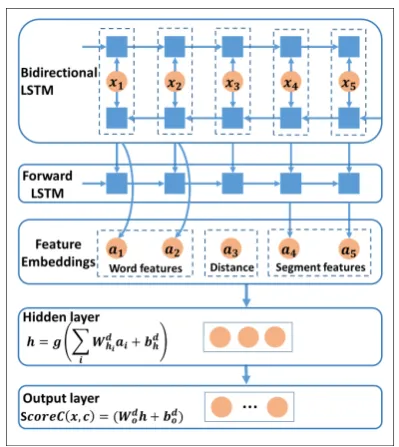
Figure 2: Architecture of the Neural Network. x1
to x5 stand for the input token of Bidirectional
LSTM.a1 toa5 stand for the feature embeddings
used in our model.
3 Neural Network Model
In this section, we describe the architecture of our neural network model in detail, which is summa-rized in Figure 2.
3.1 Input layer
In our neural network model, the words, POS tags are mapped into distributed embeddings. We represent each input token xi which is the in-put of Bidirectional LSTM by concatenating POS tag embedding epi ∈ Rde and word embedding
ewi ∈ Rde, de is the the dimensionality of em-bedding, then a linear transformation we is per-formed and passed though an element-wise acti-vation functiong:
xi =g(we[ewi;epi] +be) (3) wherexi ∈ Rde,we ∈ Rde×2de is weight matrix,
be ∈Rde is bias term. the dimensionality of input tokenxiis equal to the dimensionality of word and POS tag embeddings in our experiment, ReLU is used as our activation functiong.
3.2 Bidirectional LSTM
Given an input sequencex= (x1, . . . , xn), where
n stands for the number of words in a sentence, a standard LSTM recurrent network computes the hidden vector sequenceh = (h1, . . . , hn) in one direction.
Bidirectional LSTM processes the data in both directions with two separate hidden layers, which are then fed to the same output layer. It com-putes the forward hidden sequence −→h, the back-ward hidden sequence←−h and the output sequence
v by iterating the forward layer fromt = 1 ton, the backward layer fromt =nto1and then up-dating the output layer:
vt=−→ht+←−ht (4)
where vt ∈ Rdl is the output vector of Bidirec-tional LSTM for inputxt,−→ht∈Rdl,←−ht∈Rdl,dl is the dimensionality of LSTM hidden vector. We simply add the forward hidden vector−→htand the backward hidden vector←−httogether, which gets similar experiment result as concatenating them together with a faster speed.
The output vectors of Bidirectional LSTM are used as word feature embeddings. In addition, they are also fed into a forward LSTM network to learn segment embedding.
3.3 Segment Embedding
Contextual information of word pairs1 has been widely utilized in previous work (McDonald et al., 2005; McDonald and Pereira, 2006; Pei et al., 2015). For a dependency pair (h, m), previ-ous work divides a sentence into three parts ( pre-fix, infixandsuffix) by head wordh and modifier word m. These parts which we call segments in our work make up the context of the dependency pair(h, m).
Due to the problem of data sparseness, conven-tional graph-based models can only capture con-textual information of word pairs by using bigrams or tri-grams features. Unlike conventional mod-els, Pei et al. (2015) use distributed representa-tions obtained by averaging word embeddings in segments to represent contextual information of the word pair, which could capture richer syn-tactic and semantic information. However, their method is restricted to segment-level since their segment embedding only consider the word infor-mation within the segment. Besides, averaging operation simply treats all the words in segment equally. However, some words might carry more
1A word pair is limited to the dependency pair(h, m)in
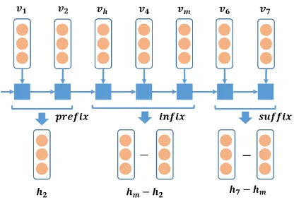
Figure 3: Illustration for learning segment embed-dings based on an extra forward LSTM network,
vh, vm and v1 to v7 indicate the output vectors
of Bidirectional LSTM for head wordh, modifier wordmand other words in sentence,hh,hm and
h1toh7indicate the hidden vectors of the forward
LSTM corresponding tovh,vmandv1tov7.
salient syntactic or semantic information and they are expected to be given more attention.
A useful property of forward LSTM is that it could keep previous useful information in their memory cell by exploiting input, output and for-get gates to decide how to utilize and update the memory of previous information. Given an in-put sequence v = (v1, . . . , vn), previous work (Sutskever et al., 2014; Vinyals et al., 2014) of-ten uses the last hidden vectorhnof the forward LSTM to represent the whole sequence. Each hid-den vectorht(1 ≤t ≤ n) can capture useful in-formation before and includingvt.
Inspired by this, we propose a method named
LSTM-Minus to learn segment embedding. We
utilize subtraction between LSTM hidden vectors to represent segment’s information. As illustrated in Figure 3, the segmentinfixcan be described as
hm−h2,hmandh2are hidden vector of the
for-ward LSTM network. The segment embedding of suffixcan also be obtained by subtraction between the last LSTM hidden vector of the sequence (h7)
and the last LSTM hidden vector ininfix(hm). For prefix, we directly use the last LSTM hidden vec-tor inprefix to represent it, which equals to sub-tract a zero embedding. When noprefixorsuffix exists, the corresponding embedding is set to zero. Specifically, we place an extra forward LSTM layer on top of the Bidirectional LSTM layer and learn segment embeddings using LSTM-Minus based on this forward LSTM. LSTM-minus en-ables our model to learn segment embeddings
from information both outside and inside the seg-ments and thus enhances our model’s ability to ac-cess to sentence-level information.
3.4 Hidden layer and output layer
As illustrated in Figure 2, we map all the feature embeddings to a hidden layer. Following Pei et al. (2015), we use direction-specific transformation to model edge direction and tanh-cube as our activa-tion funcactiva-tion:
h=g X
i
Whdiai+bdh
(5)
where ai ∈ Rdai is the feature embedding, dai indicates the dimensionality of feature embedding
ai,Whdi ∈ Rdh×dai is weight matrices which cor-responding toai,dh indicates the dimensionality of hidden layer vector,bd
h ∈Rdhis bias term.Whdi andbd
hare bound with indexd∈ {0,1}which in-dicates the direction between head and modifier.
A output layer is finally added on the top of the hidden layer for scoring dependency arcs:
ScoreC(x, c) =Wodh+bdo (6)
WhereWd
o ∈RL×dhis weight matrices,bdo ∈RL is bias term,ScoreC(x, c)∈RLis the output vec-tor,Lis the number of dependency types. Each di-mension of the output vector is the score for each kind of dependency type of head-modifier pair.
3.5 Features in our model
Previous neural network models (Pei et al., 2015; Pei et al., 2014; Zheng et al., 2013) normally set context window around a word and extract atomic features within the window to represent the con-textual information. However, context window limits their ability in detecting long-distance in-formation. Simply increasing the context window size to get more contextual information puts their model in the risk of overfitting and heavily slows down the speed.
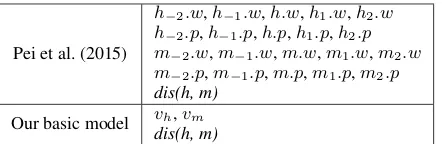
Pei et al. (2015)
h−2.w,h−1.w,h.w,h1.w,h2.w
h−2.p,h−1.p,h.p,h1.p,h2.p
m−2.w,m−1.w,m.w,m1.w,m2.w
m−2.p,m−1.p,m.p,m1.p,m2.p
dis(h, m) Our basic model vh,vm
dis(h, m)
[image:5.595.73.294.61.133.2]Table 1: Atomic features in our basic model and Pei’s 1st-order atomic model. wis short for word andpfor POS tag. h indicates head andm indi-cates modifier. The subscript represents the rela-tive position to the center word. dis(h, m)is the distance between head and modifier.vhandvm in-dicate the outputs of Bidirectional LSTM for head word and modifier word.
Table 1 lists the atomic features used in 1st-order atomic model of Pei et al. (2015) and atomic features used in our basic model. Our basic model only uses the outputs of Bidirectional LSTM for head word and modifier word, and the distance be-tween them as features. Distance features are en-coded as randomly initialized embeddings. As we can see, our basic model reduces the number of atomic features to a minimum level, making our model run with a faster speed. Based on our ba-sic model, we incorporate additional segment in-formation (prefix, infix and suffix), which further improves the effect of our model.
4 Neural Training
In this section, we provide details about training the neural network.
4.1 Max-Margin Training
We use the Max-Margin criterion to train our model. Given a training instance (x(i), y(i)), we
useY(x(i))to denote the set of all possible
depen-dency trees andy(i)is the correct dependency tree
for sentencex(i). The goal of Max Margin
train-ing is to find parametersθsuch that the difference in score of the correct tree y(i) from an incorrect
treeyˆ∈Y(x(i))is at least4(y(i),yˆ).
Score(x(i),y(i);θ)≥Score(x(i),yˆ;θ)+4(y(i),yˆ)
The structured margin loss4(y(i),yˆ)is defined
as:
4(y(i),yˆ) =
n
X
j
κ1{h(y(i), xj(i))6=h(ˆy, x(ji))}
wheren is the length of sentence x, h(y(i), x(i)
j ) is the head (with type) for thej-th word ofx(i)in
treey(i)andκis a discount parameter. The loss is
proportional to the number of word with an incor-rect head and edge type in the proposed tree.
Given a training set with sizem, The regular-ized objective function is the loss function J(θ)
including al2-norm term:
J(θ) = m1 Xm
i=1
li(θ) +λ2||θ||2
li(θ) = max
ˆ
y∈Y(x(i))(Score(x
(i),yˆ;θ)+4(y(i),yˆ))
−Score(x(i),y(i);θ) (7)
By minimizing this objective, the score of the correct tree is increased and score of the highest scoring incorrect tree is decreased.
4.2 Optimization Algorithm
Parameter optimization is performed with the di-agonal variant of AdaGrad (Duchi et al., 2011) with minibatchs (batch size = 20) . The param-eter update for thei-th parameterθt,i at time step
tis as follows:
θt,i=θt−1,i−qPtα τ=1g2τ,i
gt,i (8)
whereαis the initial learning rate (α = 0.2in our experiment) and gτ ∈ R|θi| is the subgradient at time stepτ for parameterθi.
To mitigate overfitting, dropout (Hinton et al., 2012) is used to regularize our model. we apply dropout on the hidden layer with 0.2 rate.
4.3 Model Initialization&Hyperparameters
The following hyper-parameters are used in all experiments: word embedding size = 100, POS tag embedding size = 100, hidden layer size = 200, LSTM hidden vector size = 100, Bidirec-tional LSTM layers = 2, regularization parameter
λ=10−4.
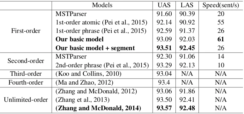
Models UAS LAS Speed(sent/s)
First-order
MSTParser 91.60 90.39 20
1st-order atomic (Pei et al., 2015) 92.14 90.92 55 1st-order phrase (Pei et al., 2015) 92.59 91.37 26
Our basic model 93.09 92.03 61
Our basic model + segment 93.51 92.45 26
Second-order MSTParser2nd-order phrase (Pei et al., 2015) 93.29 92.1392.30 91.06 1410 Third-order (Koo and Collins, 2010) 93.04 N/A N/A Fourth-order (Ma and Zhao, 2012) 93.4 N/A N/A
Unlimited-order (Zhang and McDonald, 2012)(Zhang et al., 2013) 93.06 91.8693.50 92.41 N/AN/A
[image:6.595.104.495.61.243.2](Zhang and McDonald, 2014) 93.57 92.48 N/A
Table 2: Comparison with previous graph-based models on Penn-YM.
5 Experiments
In this section, we present our experimental setup and the main result of our work.
5.1 Experiments Setup
We conduct our experiments on the English Penn Treebank (PTB) and the Chinese Penn Treebank (CTB) datasets.
For English, we follow the standard splits of PTB3. Using section 2-21 for training, section 22 as development set and 23 as test set. We con-duct experiments on two different constituency-to-dependency-converted Penn Treebank data sets. The first one, Penn-YM, was created by the Penn2Malt tool2based on Yamada and Matsumoto (2003) head rules. The second one, Penn-SD, use Stanford Basic Dependencies (Marneffe et al., 2006) and was converted by version 3.3.03 of the Stanford parser. The Stanford POS Tagger (Toutanova et al., 2003) with ten-way jackknifing of the training data is used for assigning POS tags (accuracy≈97.2%).
For Chinese, we adopt the same split of CTB5 as described in (Zhang and Clark, 2008). Follow-ing (Zhang and Clark, 2008; Dyer et al., 2015; Chen and Manning, 2014), we use gold segmen-tation and POS tags for the input.
5.2 Experiments Results
We first make comparisons with previous graph-based models of different orders as shown in
Ta-2http://stp.lingfil.uu.se/nivre/
research/Penn2Malt.html
3http://nlp.stanford.edu/software/
lex-parser.shtml
ble 2. We use MSTParser4for conventional first-order model (McDonald et al., 2005) and second-order model (McDonald and Pereira, 2006). We also include the results of conventional high-order models (Koo and Collins, 2010; Ma and Zhao, 2012; Zhang and McDonald, 2012; Zhang et al., 2013; Zhang and McDonald, 2014) and the neu-ral network model of Pei et al. (2015). Different from typical high-order models (Koo and Collins, 2010; Ma and Zhao, 2012), which need to extend their decoding algorithm to score new types of higher-order dependencies. Zhang and McDonald (2012) generalized the Eisner algorithm to handle arbitrary features over higher-order dependencies and controlled complexity via approximate decod-ing with cube prundecod-ing. They further improve their work by using perceptron update strategies for in-exact hypergraph search (Zhang et al., 2013) and forcing inference to maintain both label and struc-tural ambiguity through a secondary beam (Zhang and McDonald, 2014).
Following previous work, UAS (unlabeled at-tachment scores) and LAS (labeled atat-tachment scores) are calculated by excluding punctuation5. The parsing speeds are measured on a workstation with Intel Xeon 3.4GHz CPU and 32GB RAM which is same to Pei et al. (2015). We measure the parsing speeds of Pei et al. (2015) according to their codes6and parameters.
On accuracy, as shown in table 2, our
4http://sourceforge.net/projects/ mstparser
5Following previous work, a token is a punctuation if its
POS tag is{“ ” : , .}
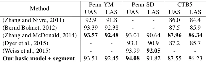
Method UASPenn-YMLAS UASPenn-SDLAS UASCTB5LAS (Zhang and Nivre, 2011) 92.9 91.8 - - 86.0 84.4 (Bernd Bohnet, 2012) 93.39 92.38 - - 87.5 85.9 (Zhang and McDonald, 2014) 93.57 92.48 93.01 90.64 87.96 86.34
(Dyer et al., 2015) - - 93.1 90.9 87.2 85.7 (Weiss et al., 2015) - - 93.99 92.05 -
[image:7.595.119.482.61.171.2]-Our basic model + segment 93.51 92.45 94.08 91.82 87.55 86.23
Table 3: Comparison with previous state-of-the-art models on Penn-YM, Penn-SD and CTB5.
basic model outperforms previous first-order graph-based models by a substantial margin, even outperforms Zhang and McDonald (2012)’s unlimited-order model. Moreover, incorporating segment information further improves our model’s accuracy, which shows that segment embeddings do capture richer contextual information. By using segment embeddings, our improved model could be comparable to high-order graph-based models7. With regard to parsing speed, our model also shows advantage of efficiency. Our model uses only first-order factorization and requires O(n3)
time to decode. Third-order model requiresO(n4)
time and fourth-order model requiresO(n5) time.
By using approximate decoding, the unlimited-order model of Zhang and McDonald (2012) re-quiresO(k·log(k)·n3) time, wherekis the beam
size. The computational cost of our model is the lowest among graph-based models. Moreover, al-though using LSTM requires much computational cost. However, compared with Pei’s 1st-order model, our model decreases the number of atomic features from 21 to 3, this allows our model to re-quire a much smaller matrix computation in the scoring model, which cancels out the extra compu-tation cost introduced by the LSTM compucompu-tation. Our basic model is the fastest among first-order and second-order models. Incorporating segment information slows down the parsing speed while it is still slightly faster than conventional first-order model. To compare with conventional high-order models on practical parsing speed, we can make an indirect comparison according to Zhang and McDonald (2012). Conventional first-order model is about 10 times faster than Zhang and
McDon-7Note that our model can’t be strictly comparable with
third-order model (Koo and Collins, 2010) and fourth-order model (Ma and Zhao, 2012) since they are unlabeled model. However, our model is comparable with all the three unlimited-order models presented in (Zhang and McDon-ald, 2012), (Zhang et al., 2013) and (Zhang and McDonMcDon-ald, 2014), since they all are labeled models as ours.
Method Peen-YM Peen-SD CTB5 Average 93.23 93.83 87.24
LSTM-Minus 93.51 94.08 87.55
Table 4: Model performance of different way to learn segment embeddings.
ald (2012)’s unlimited-order model and about 40 times faster than conventional third-order model, while our model is faster than conventional first-order model. Our model should be much faster than conventional high-order models.
We further compare our model with previous state-of-the-art systems for English and Chinese. Table 3 lists the performances of our model as well as previous state-of-the-art systems on on Penn-YM, Penn-SD and CTB5. We compare to conven-tional state-of-the-art graph-based model (Zhang and McDonald, 2014), conventional state-of-the-art transition-based model using beam search (Zhang and Nivre, 2011), transition-based model combining graph-based approach (Bernd Bohnet, 2012) , transition-based neural network model us-ing stack LSTM (Dyer et al., 2015) and transition-based neural network model using beam search (Weiss et al., 2015). Overall, our model achieves competitive accuracy on all three datasets. Al-though our model is slightly lower in accuarcy than unlimited-order double beam model (Zhang and McDonald, 2014) on Penn-YM and CTB5, our model outperforms their model on Penn-SD. It seems that our model performs better on data sets with larger label sets, given the number of la-bels used in Penn-SD data set is almost four times more than Penn-YM and CTB5 data sets.
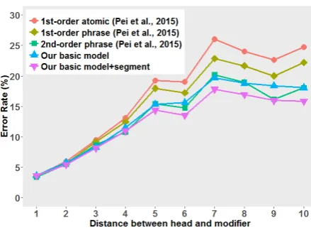
Figure 4: Error rates of different distance between head and modifier on Peen-YM.
To make comparison as fair as possible, we let two models have almost the same number parameters. Table 4 lists the UAS of two methods on test set. As we can see, LSTM-Minus shows better per-formance because our method further incorporates more sentence-level information into our model.
5.3 Impact of Network Structure
In this part, we investigate the impact of the com-ponents of our approach.
LSTM Recurrent Network
To evaluate the impact of LSTM, we make er-ror analysis on Penn-YM. We compare our model with Pei et al. (2015) on error rates of different distance between head and modifier.
As we can see, the five models do not show much difference for short dependencies whose dis-tance less than three. For long dependencies, both our two models show better performance com-pared with the 1st-order model of Pei et al. (2015), which proves that LSTM can effectively capture long-distance dependencies. Moreover, our mod-els and Pei’s 2nd-order phrase model both im-prove accuracy on long dependencies compared with Pei’s 1st-order model, which is in line with our expectations. Using LSTM shows the same effect as high-order factorization strategy. Com-pared with 2nd-order phrase model of Pei et al. (2015), our basic model occasionally performs worse in recovering long distant dependencies. However, this should not be a surprise since higher order models are also motivated to recover long-distance dependencies. Nevertheless, with the in-troduction of LSTM-minus segment embeddings, our model consistently outperforms the 2nd-order
phrase model of Pei et al. (2015) in accuracies of all long dependencies. We carried out significance test on the difference between our and Pei’s mod-els. Our basic model performs significantly better than all 1st-order models of Pei et al. (2015) (t-test with p<0.001) and our basic+segment model (still a 1st-order model) performs significantly bet-ter than their 2nd-order phrase model (t-test with p<0.001) in recovering long-distance dependen-cies.
Initialization of pre-trained word embeddings
We further analyze the influence of using pre-trained word embeddings for initialization. with-out using pretrained word embeddings, our im-proved model achieves 92.94% UAS / 91.83% LAS on Penn-YM, 93.46% UAS / 91.19% LAS on Penn-SD and 86.5% UAS / 85.0% LAS on CTB5. Using pre-trained word embeddings can obtain around 0.5%∼1.0% improvement.
6 Related work
Dependency parsing has gained widespread inter-est in the computational linguistics community. There are a lot of approaches to solve it. Among them, we will mainly focus on graph-based de-pendency parsing model here. Dede-pendency tree factorization and decoding algorithm are neces-sary for graph-based models. McDonald et al. (2005) proposed the first-order model which de-composes a dependency tree into its individual edges and use a effective dynamic programming algorithm (Eisner, 2000) to decode. Based on first-order model, higher-first-order models(McDonald and Pereira, 2006; Carreras, 2007; Koo and Collins, 2010; Ma and Zhao, 2012) factor a dependency tree into a set of high-order dependencies which bring interactions between head, modifier, siblings and (or) grandparent into their model. However, for above models, scoring new types of higher-order dependencies requires extensions of the un-derlying decoding algorithm, which also requires higher computational cost. Unlike above models, unlimited-order models (Zhang and McDonald, 2012; Zhang et al., 2013; Zhang and McDonald, 2014) could handle arbitrary features over higher-order dependencies by generalizing the Eisner al-gorithm.
combinations via a novel activation function, al-lowing their model to use a set of atomic features instead of millions of hand-crafted features.
Different from previous work, which is sensi-tive to local state and accesses to larger context by higher-order factorization. Our model makes pars-ing decisions on a global perspective with first-order factorization, avoiding the expensive com-putational cost introduced by high-order factoriza-tion.
LSTM network is heavily utilized in our model. LSTM network has already been explored in transition-based dependency parsing. Dyer et al. (2015) presented stack LSTMs with push and pop operations and used them to imple-ment a state-of-the-art transition-based depen-dency parser. Ballesteros et al. (2015) replaced lookup-based word representations with character-based representations obtained by Bidirectional LSTM in the continuous-state parser of Dyer et al. (2015), which was proved experimentally to be useful for morphologically rich languages.
7 Conclusion
In this paper, we propose an LSTM-based neural network model for graph-based dependency pars-ing. Utilizing Bidirectional LSTM and segment embeddings learned by LSTM-Minus allows our model access to sentence-level information, mak-ing our model more accurate in recovermak-ing long-distance dependencies with only first-order factor-ization. Experiments on PTB and CTB show that our model could be competitive with conventional high-order models with a faster speed.
Acknowledgments
This work is supported by National Key Ba-sic Research Program of China under Grant No.2014CB340504 and National Natural Science Foundation of China under Grant No.61273318. The Corresponding author of this paper is Baobao Chang.
References
Miguel Ballesteros, Chris Dyer, and Noah A. Smith. 2015. Improved transition-based parsing by model-ing characters instead of words with lstms. In Pro-ceedings of the 2015 Conference on Empirical Meth-ods in Natural Language Processing, EMNLP 2015, Lisbon, Portugal, September 17-21, 2015, pages 349–359.
Jonas Kuhn Bernd Bohnet. 2012. The best of both worlds: a graph-based completion model for transition-based parsers. Conference of the Euro-pean Chapter of the Association for Computational Linguistics.
Xavier Carreras. 2007. Experiments with a higher-order projective dependency parser. In EMNLP-CoNLL, pages 957–961.
Danqi Chen and Christopher D. Manning. 2014. A fast and accurate dependency parser using neural net-works. InProceedings of the 2014 Conference on Empirical Methods in Natural Language Process-ing, pages 740–750.
John Duchi, Elad Hazan, and Yoram Singer. 2011. Adaptive subgradient methods for online learning and stochastic optimization. The Journal of Ma-chine Learning Research, pages 2121–2159. Chris Dyer, Miguel Ballesteros, Wang Ling, Austin
Matthews, and Noah A. Smith. 2015. Transition-based dependency parsing with stack long short-term memory. In Proceedings of the 53rd Annual Meeting of the Association for Computational Lin-guistics, pages 334–343.
Jason Eisner. 2000. Bilexical Grammars and their Cubic-Time Parsing Algorithms. Springer Nether-lands.
David Graff, Junbo Kong, Ke Chen, and Kazuaki Maeda. 2003. English gigaword. Linguistic Data Consortium, Philadelphia.
Geoffrey E Hinton, Nitish Srivastava, Alex Krizhevsky, Ilya Sutskever, and Ruslan R Salakhutdinov. 2012. Improving neural networks by preventing co-adaptation of feature detectors. arXiv preprint arXiv:1207.0580.
Terry Koo and Michael Collins. 2010. Efficient third-order dependency parsers. In Proceedings of the 48th Annual Meeting of the Association for Com-putational Linguistics, pages 1–11. Association for Computational Linguistics.
Wang Ling, Chris Dyer, Alan Black, and Isabel Trancoso. 2015. Two/too simple adaptations of word2vec for syntax problems. In Proceedings of the 2015 Conference of the North American Chap-ter of the Association for Computational Linguistics: Human Language Technologies.
Xuezhe Ma and Hai Zhao. 2012. Fourth-order de-pendency parsing. In COLING 2012, 24th Inter-national Conference on Computational Linguistics, Proceedings of the Conference: Posters, 8-15 De-cember 2012, Mumbai, India, pages 785–796. Marie Catherine De Marneffe, Bill Maccartney, and
Christopher D. Manning. 2006. Generating typed dependency parses from phrase structure parses.
Ryan T McDonald and Fernando CN Pereira. 2006. Online learning of approximate dependency parsing algorithms. InEACL. Citeseer.
Ryan McDonald, Koby Crammer, and Fernando Pereira. 2005. Online large-margin training of de-pendency parsers. In Proceedings of the 43rd an-nual meeting on association for computational lin-guistics, pages 91–98. Association for Computa-tional Linguistics.
Wenzhe Pei, Tao Ge, and Baobao Chang. 2014. Max-margin tensor neural network for chinese word seg-mentation. InProceedings of the 52nd Annual Meet-ing of the Association for Computational LMeet-inguistics (Volume 1: Long Papers), pages 293–303.
Wenzhe Pei, Tao Ge, and Baobao Chang. 2015. An effective neural network model for graph-based de-pendency parsing. In Proceedings of the 53rd An-nual Meeting of the Association for Computational Linguistics, pages 313–322.
Ilya Sutskever, Oriol Vinyals, and Quoc V. Le. 2014. Sequence to sequence learning with neural net-works. InAdvances in Neural Information Process-ing Systems 27: Annual Conference on Neural In-formation Processing System, pages 3104–3112. Kristina Toutanova, Dan Klein, Christopher D
Man-ning, and Yoram Singer. 2003. Feature-rich part-of-speech tagging with a cyclic dependency network. InProceedings of the 2003 Conference of the North American Chapter of the Association for Computa-tional Linguistics on Human Language Technology-Volume 1, pages 173–180. Association for Compu-tational Linguistics.
Oriol Vinyals, Lukasz Kaiser, Terry Koo, Slav Petrov, Ilya Sutskever, and Geoffrey E. Hinton. 2014. Grammar as a foreign language. CoRR, abs/1412.7449.
David Weiss, Chris Alberti, Michael Collins, and Slav Petrov. 2015. Structured training for neural net-work transition-based parsing. InProceedings of the 53rd Annual Meeting of the Association for Compu-tational Linguistics.
Hiroyasu Yamada and Yuji Matsumoto. 2003. Statis-tical dependency analysis with support vector ma-chines. InProceedings of IWPT, volume 3, pages 195–206.
Yue Zhang and Stephen Clark. 2008. A tale of two parsers: Investigating and combining graph-based and transition-based dependency parsing. In 2008 Conference on Empirical Methods in Natural Lan-guage Processing, pages 562–571.
Hao Zhang and Ryan T. McDonald. 2012. Generalized higher-order dependency parsing with cube prun-ing. InProceedings of the 2012 Joint Conference on Empirical Methods in Natural Language Process-ing and Computational Natural Language LearnProcess-ing, pages 320–331.
Hao Zhang and Ryan T. McDonald. 2014. Enforc-ing structural diversity in cube-pruned dependency parsing. In Proceedings of the 52nd Annual Meet-ing of the Association for Computational LMeet-inguis- Linguis-tics, pages 656–661.
Yue Zhang and Joakim Nivre. 2011. Transition-based dependency parsing with rich non-local features. In
The 49th Annual Meeting of the Association for Computational Linguistics: Human Language Tech-nologies, pages 188–193.
Hao Zhang, Liang Huang Kai Zhao, and Ryan Mcdon-ald. 2013. Online learning for inexact hypergraph search. Proceedings of Emnlp.