Quantum Error Correction with Biased Noise

(1)

Quantum Error Correction with Biased Noise

Thesis by

Peter Brooks

In Partial Fulfillment of the Requirements for the Degree of

Doctor of Philosophy

California Institute of Technology Pasadena, California

2013

(2)

Copyright notice. Chapters 2 and 3 contain material from [1] and [2], respectively, which are copyrighted by the American Physical Society.

The remaining material is

(3)

(4)

Acknowledgements

I would first like to thank my advisor, John Preskill. John has been an exemplary mentor and role model, with a broad and deep knowledge of physics, an insightful mind, and a ready smile. I could not have asked for a better advisor, and I am immensely proud to have been his student.

I am been extremely lucky to have been blessed with a number of extraordinarily thoughtful mentors who have guided my journey through physics and life. I am especially grateful for guidance and support from Alexei Kitaev, Jim Harrington, Pat Burchat, Ian Fisher, Blas Cabrera and Fritz DeJongh. Most of all I would like to thank Bruce Keyzer, whose inspiring teaching instilled in me an incurable passion for physics and set this entire course in motion.

I owe much of what I have learned to conversations with collaborators and friends, especially Adam Paetznick, Cody Jones, Jeongwan Haah, Isaac Kim, and the entire IQI(M!) group at Caltech. And I could not have survived a Ph.D. without the help of Ann Harvey, to whom I am eternally grateful.

(5)

Abstract

Quantum computing o↵ers powerful new techniques for speeding up the calculation of many clas-sically intractable problems. Quantum algorithms can allow for the efficient simulation of physical systems, with applications to basic research, chemical modeling, and drug discovery; other algo-rithms have important implications for cryptography and internet security.

At the same time, building a quantum computer is a daunting task, requiring the coherent manipulation of systems with many quantum degrees of freedom while preventing environmental noise from interacting too strongly with the system. Fortunately, we know that, under reasonable assumptions, we can use the techniques of quantum error correction and fault tolerance to achieve an arbitrary reduction in the noise level.

In this thesis, we look at how additional information about the structure of noise, or “noise bias,” can improve or alter the performance of techniques in quantum error correction and fault tolerance. In Chapter 2, we explore the possibility of designing certain quantum gates to be extremely robust with respect to errors in their operation. This naturally leads to structured noise where certain gates can be implemented in a protected manner, allowing the user to focus their protection on the noisier unprotected operations.

In Chapter 3, we examine how to tailor error-correcting codes and fault-tolerant quantum circuits in the presence of dephasing biased noise, where dephasing errors are far more common than bit-flip errors. By using an appropriately asymmetric code, we demonstrate the ability to improve the amount of error reduction and decrease the physical resources required for error correction.

(6)

List of Figures

1.1 TransversalH and CNOT gates. . . 15

1.2 Preparation of a verified 4-qubit cat state. . . 16

1.3 Steane error correction. . . 16

2.1 The energyE(✓) of the 0-⇡qubit. . . 19

2.2 Two-rung superconducting circuit underlying the 0-⇡qubit. . . 20

2.3 The circuit for the 0-⇡qubit. . . 23

2.4 An unprotected phase gate. . . 25

2.5 A protected phase gate. . . 26

2.6 An e↵ective Josephson junction. . . 26

2.7 The profile of the tunable Josephson couplingJ(t) in the execution of the protected phase gate. . . 27

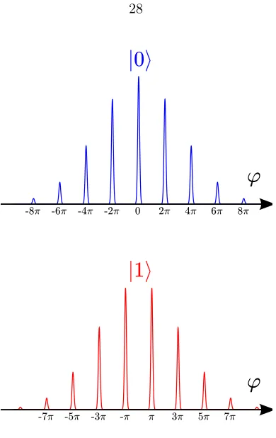
2.8 Coupling the qubit to the oscillator prepares a grid state in'space, a superposition of narrowly peaked functions governed by a broad envelope function. . . 28

2.9 Ideal codewords of the continuous variable code. . . 38

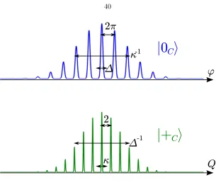
2.10 Approximate codewords of the continuous variable code. . . 40

2.11 The estimated gate error_|⌘"|(on a log scale) as a function of the rotation error", for  2_{= 40. . . .} ₅₀

2.12 The estimated gate error|⌘"|(on a log scale) as a function of the rotation error", for  2_{= 80. . . .} ₅₁

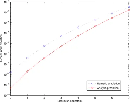
2.13 The numerically computed and analytic prediction for the diamond-norm deviation from the ideal phase gate, for 2₌p_L/C_{= 80,} 2₌p_J

0C= 8, and⌧J/C = 80 . 58

(11)

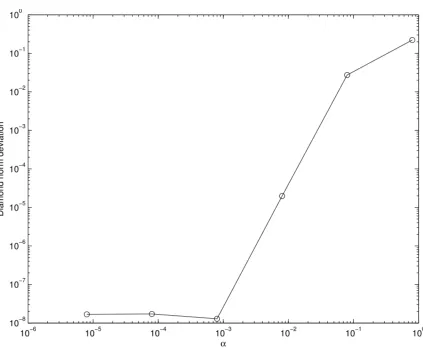
2.15 The minimum diamond-norm deviation of the protected phase gate from the ideal gate, as a function of the oscillator’s anharmonicity parameter↵= LpL/C. Here,

as in Figure 2.13,pL/C = 80 andpJ0C= 8. . . 66

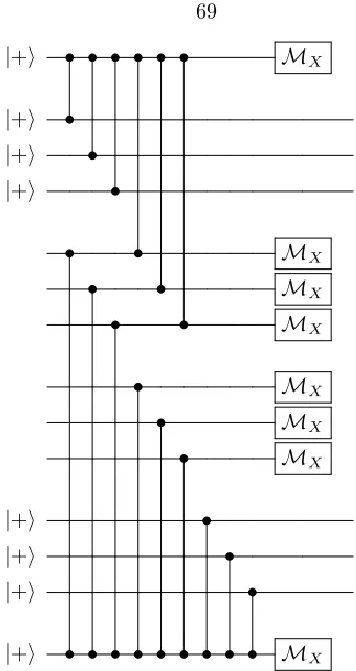
2.16 Logical CNOT gate acting on two blocks of the repetition code, shown here for code lengthn= 3. . . 69

2.17 Adiabatic switch. ForpL/C 1, the e↵ective Josephson energyJe↵ of the switch is depends sensitively on circuit parameters. . . 72

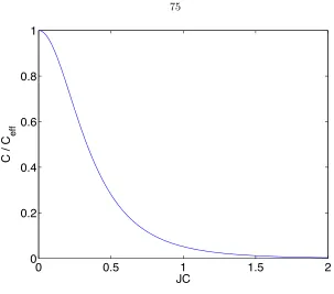
2.18 The inverse e↵ective capacitance of a Josephson junction as a function ofJC. . . 75

2.19 The e↵ective Josephson parameter of the adiabatic switch as a function of JC for p L/C = 40. . . 77

3.1 Bacon-Shor qubits arranged in ann_⇥mlattice. . . 100

3.2 Bacon-Shor stabilizers. . . 100

3.3 Z measurement performed withX measurement and an ancilla. . . 102

3.4 Gadget for a single row of the non-destructive_ML Z measurement . . . 104

3.5 Four versions of the CNOT gadget. . . 107

3.6 One-bit teleportation circuit. . . 107

3.7 Teleported CNOT gate. . . 108

3.8 Arrangement of Bacon-Shor qubits for geometrically local computation for 3⇥5 code block. . . 119

3.9 Optimal CNOT logical error rate versus physical error rate for various values of the bias. . . 123

3.10 Optimal CNOT logical error rate versus required number of physical gates for a phys-ical error rate"= 10 4_{at various values of the bias. . . 125}

3.11 Optimal CNOT logical error rate versus physical error rate for various values of the bias, where two-qubit physical gates are assumed to be geometrically local. . . 126

(12)

3.13 Bacon-Shor block size vs optimal (in number of gates) CNOT logical error rate for geometrically local asymmetric Bacon-Shor codes at various values of the bias, for a

physical error rate"= 10 4_{. . . 128}

3.14 Optimal CNOT logical error rate versus required number of gates for geometrically local asymmetric Bacon-Shor codes, assuming a physical error rate"= 10 4_{, bias 10}4_, and various rates of the measurement error rate"M. . . 129

3.15 Injection error probability for the optimal geometrically local Bacon-Shor codes . . . . 130

3.16 Output error probability aftern levels of |Tidistillation, with the values of "in and "CSS taken from the optimal values of Figure 3.15, for"= 10 4 and various biases. . . 132

4.1 Distillation circuit for the state_|i_iand equivalent circuit transformations. . . 141

4.2 Alternate distillation circuit for the state_|i_i. . . 141

4.3 Teleported circuits for the Cli↵ord gatesQandS. . . 143

4.4 Distillation circuit for the state_|T_iand equivalent circuit transformations. . . 145

4.5 Teleported circuit for the non-Cli↵ord gatesT. . . 146

4.6 Distillation circuit for the state|Hi. . . 152

4.7 Circuit consuming two copies of the magic state|Hito perform a controlled-H gate. . 153

4.8 Output error rate"outfrom Equation (4.92), versus input error rate"infor distillation based on the [[15,1,3]] Reed-Muller code, for three di↵erent values of the Cli↵ord operation failure ratep. The dashed line represents the result of no distillation. . . 163

4.9 Output error rate "out from Equation (4.92) after n rounds of distillation, for dis-tillation based on the [[15,1,3]] Reed-Muller code and various values of the Cli↵ord operation failure ratep, starting from a near-threshold input error rate of"(0)_{= 0.15. 164} 4.10 Number of ways to combine one or two non-transverse faults and up to one additional non-transverse fault to create an encoded error on a particular output qubit, averaged over choice of output qubit, for various Bravyi-Haah code sizesk. . . 167

(13)

4.12 Output error rate"out from Equations (4.94) and (4.96) versus input error rate"infor

distillation based on various Jones and Bravyi-Haah codes, forp= 10 12_{. The dashed}

line represents the result of no distillation. . . 170 4.13 Output error rate"out from Equations (4.94) and (4.96) versus input error rate"infor

distillation based on various Jones and Bravyi-Haah codes, forp= 10 4_{. The dashed}

line represents the result of no distillation. . . 171 4.14 Output error probability"outas a function of number of rounds of distillation, for five

di↵erent distillation codes, starting from"in= 0.01 and withp= 10 10. . . 172

(14)

Chapter 1

Background

Plans are worthless, but planning is everything.

–Dwight D. Eisenhower [3]

This chapter aims to give a brief introduction to the terminology and techniques of quantum computing, error correction and fault tolerance, with particular focus on material relevant for the rest of the thesis. For a fuller overview see [4–6].

1.1 Overview

It was first noted by Feynman [7, 8] and Deutsch [9, 10] that simulating quantum systems on a classical computer seems to require a calculation whose time scales exponentially with the size of the simulated system; whereas the nature is able to efficiently “simulate” such a system by the system itself. Therefore a computer designed to take full advantage of laws of nature, in particular the laws of quantum mechanics, might o↵er a fundamentally more powerful mode of computation than a classical computer, o↵ering a counter-argument to the strong Church–Turing hypothesis [11,12]. This intuition was further strengthened by the discovery of quantum algorithms with no classical analogue, especially by Shor’s discovery of polynomial-time algorithms for finding the factors of prime numbers and computing discrete logarithms [13]. Since then, more and more quantum algorithms have been found, with applications ranging from searches of unstructured databases [14] to simulations of quantum field theories [15, 16] and molecular properties [17–19].

(15)

many di↵erent states, and, by a carefully designed pattern of interference, paths corresponding to the correct answer to the calculation interfere constructively while paths corresponding to wrong answers interfere destructively and cancel out to some degree. In many cases, the entanglement of di↵erent subsystems of the quantum computer with each other plays a key role in quantum algorithms.

A quantum state is a far more fragile state than its classical counterpart. It can be destroyed not only by disturbing the system directly, but also by measuring the system. Just as the inter-ference fringes of the double-slit experiment are destroyed if it is possible to learn which path the particle has passed through, the interference necessary for a quantum calculation can be destroyed if information about the state of the computer leaks into its environment. Nevertheless, the theory of quantum error correcting codes and quantum fault tolerance have shown that, in principle, a suf-ficiently isolated quantum calculation can be protected against errors arising from its environment to an arbitrary degree. This is achieved by encoding the state of the calculation non-locally in a quantum error correcting code. Once encoded, the environment cannot access the computational state without measuring an extensive number of bare systems.

(16)

1.2 Quantum computation

The state of a classical computer is a string ofbits, each of which can take one of two values, 0 or 1. Equivalently, its state is a vector over the binary field Z2. A computation is a process which

maps bit strings to other bit strings, either in a deterministic way, or with some probability. We can decompose any classical computation into a sequence of fundamental operations, called gates, and a connectivity diagram, a wiring, indicating how the outputs of one gate are mapped into the inputs of future gates.

The fundamental unit of quantum information is the quantum bit, or qubit. Unlike its classical analogue, the bit, which can take two values, the qubit can be described by a vector

| i=a|0i+b|1i, (1.1)

where the componentsaand b are both complex numbers, called amplitudes. This state is called normalized if

| i =h | i=|a|2+|b|2, (1.2) the norm of the qubit, is equal to 1.

We can perform a measurement on our qubit, which returns a classical bit, 0 or 1. The “logical basis” or “computational basis” measurement returns the value 0 with probability |a|2 and the value 1 with probability|b|2. After the measurement, if we received the result 0, then we will find our qubit in the state|0i, and if we received the result 1, then we will find our qubit in the state |1i. In e↵ect, the measurement projects the state of the qubit onto the two basis states, |0iand |1_i. The normalization condition means that we will always find our qubit in one of the two states. We can also perform a measurement in a di↵erent basis. One important basis is the “dual basis” measurement, which projects onto the two states

|+i= p1

2(|0i+|1i) (1.3)

| i= p1

2(|0i |1i), (1.4)

(17)

project onto any orthogonal set of basis states.

The state of the qubit can be reversibly manipulated by applying a unitary operation— a linear map from one state_| _ito a new state_|'_i. For a single qubit, such a map can be thought of as a 2_⇥2 complex matrix

U = 0 B B B @ a b c d 1 C C C

A, (1.5)

satisfyingU†U =I, whereU† is the Hermetian adjoint

U† = 0 B B B @

a⇤ c⇤

b⇤ _d⇤ 1 C C C

A, (1.6)

andIis the identity matrix

I= 0 B B B @ 1 0 0 1 1 C C C

A, (1.7)

which maps any state| ito itself.

The state ofn qubits requires 2n _{complex numbers to specify, one for each of the 2}n _classical

length-nbit strings, just as a probabilistic state ofnbits would require 2n _{real numbers}

(probabil-ities) to describe. Some states, such as the state 1

2 |00i+|01i+|10i+|11i =|+i ⌦|+i, (1.8) can be decomposed into states on each individual qubit; such a state is called a product state. Other states, such as the “EPR pair” [20] state

1 p

2 |00i+|11i , (1.9)

cannot be decomposed in this way, and are called entangled states.

(18)

for states_|↵_i=P_iai|siiand| i=Pibi|siias

h↵| i=X

i,j

a⇤ibjhsi|sji=

X

i

c⇤idi. (1.10)

The Hermetian adjoint, defined earlier, is the adjoint with respect to this inner product, so that the “ket”U_| _icorresponds to the “bra”_h _|U†_{. In this notation, we can decompose any operator} as

X

i

|↵iih i|, (1.11)

which acts on the state_| _ias X

i

|↵iih i|

!

| i=X

i

h i| i|↵ii. (1.12)

When considering a quantum system with two subsystems_HA⌦HB, we cannot always describe

the state of one subsystem_HA as some “pure state”| i. For example, the EPR state

1 p

2 |00i+|11i ,

from the perspective of an observer of one half of the system, looks like a probabilistic (non-coherent) mixture of|0iand|1i, each with probability 1/2. To describe such a state, we can introduce the density matrix description of a state. A pure state| ihas density matrix ⇢=| ih |. For a state P

a| ai ⌦| ai, the “reduced state” on subsystem HA has density operator ⇢ = Pa| aih a|. A

unitary operator acts on a density matrix⇢as

(19)

1.2.1 The Pauli operators

It is helpful to understand a system of qubits by studying how various operators act on the states of the system. One useful set of states are the Pauli matrices

X= 0 B B B @ 1 1 1 C C C A Y =

0 B B B @ i i 1 C C C A Z=

0 B B B @ 1 1 1 C C C

A, (1.14)

where by convention the empty entries are zeros. In bra-ket notation they can be written as

X=|0ih1|+|1ih0| Y = i|0ih1|+i|1ih0| Z=|0ih0| |1ih1|, (1.15)

We can describe the computational basis measurement as a measurement of the eigenvalues ofZ, and the dual basis measurement corresponds to measuring the eigenvalues ofX; we could similarly measure the eigenvalues of theY operation. For a qubit consisting of a particle’s spin, these three measurements correspond to measuring the spin along thex,y andz axes.

Each Pauli operation describes a useful basis, defined by its eigenvectors. The eigenvectors of Z are|0iand|1i, while the eigenvalues ofX are given by

|+_i=p1

2 |0i+|1i (1.16)

| i=p1

2 |0i |1i , (1.17)

withX_|+_i=_|+_iandX_| _i= _| _i. The eigenvalues ofY are given by

|i_i=p1

2 |0i+i|1i (1.18)

| ii=p1

2 |0i i|1i , (1.19)

withY_|±i_i=_±|±i_i.

The Pauli matrices anti commute with each other, obeying

(20)

(where 1 =X, 2=Y, and 3=Z.) They form a group, in the sense that any product of Pauli

operators is itself a Pauli operator, up to an irrelevant phase. The Pauli group onn qubits, _Pn,

is any operation which can be written as the tensor product of single-qubit Pauli operators and identity operators.

More generally, we can measure the eigenvalues of any operatorA whose eigenvalues are real; such an operator is called Hermetian and obeysA† =A. If two operatorsA and B commute, so that

[A, B] =AB BA= 0, (1.21)

then both of their eigenvalues can be measured simultaneously. Similarly, all of the eigenvalues of a set of mutually commuting operators may be measured simultaneously. In general, operators may neither commute nor anticommute.

1.2.2 The Cli

↵

ord group

Another useful group of operations are the Cli↵ord group of operationsC1, which are defined to be

the operations which transform Pauli operations into Pauli operations:

CP C†2Pn forP 2Pn, C2C1. (1.22)

Examples of Cli↵ord operations include the Hadamard operation

H =p1 2

0 B B B @

1 1 1 1

1 C C C

A, (1.23)

which exchanges the logical and dual bases; the phase gate

S= 0 B B B @ 1

i 1 C C C

(21)

and the two-qubit controlled-NOT or CNOT gate

CNOT = • = 0 B B B B B B B B B B B B @ 1 1 1 1 1 C C C C C C C C C C C C A , (1.25)

which in the logical basis flips the value of the second qubit based on the value of the first. In fact, any operation in the Cli↵ord group can be decomposed into these elementary operations. Another useful Pauli operation is the controlled-Z operation

CZ = • • = 0 B B B B B B B B B B B B @ 1 1 1 1 1 C C C C C C C C C C C C A . (1.26)

In terms of their e↵ect on the Pauli operations, these Cli↵ord operations can be described as

H :X !Z Y _!Y

Z !X,

(1.27)

S:X_!Y Y !X

Z_!Z,

(22)

and

CNOT :IX!IX IZ!ZZ

XI_!XX ZI _!ZI, (1.29)

where the rest of the CNOT relations follow from linearity.

While the Cli↵ord operations are insufficient for universal computation, they are useful for describing error correcting circuits.

1.2.3 Universal computation

We would like to be able to implement or approximate an arbitrary unitary operationU, to arbitrary precision ✏, by decomposing it into a sequence of fundamental operations or gates, just as an ordinary computation can be decomposed into logic gates from a finite set. The Cli↵ord operations of Section 1.2.2 are insufficient for the task, because they generate only a finite group of unitaries. It can be shown [4] that the Cli↵ord operations together with any one non-Cli↵ord single qubit gate is sufficient for universality. Moreover, an✏-approximation to a unitaryU can be constructed efficiently [6, 21–23]. One common choice for a universal set of gates is

C1[{T}, (1.30)

whereT is the gate

T = 0 B B B @ 1

ei⇡/4

1 C C C

A. (1.31)

A more streamlined set is

{H, T,CNOT_}, (1.32) which is universal because H, S = T2 _{and CNOT complete the Cli}_↵_{ord group, while} _T _is

(23)

1.3 Error correcting codes

Error correcting codes, both classical and quantum, are methods of storing information redundantly so that, even though a part of the information has been corrupted or lost, the stored information can be recovered with high probability.

1.3.1 Classical error correction

The simplest classical error correcting code is the repetition code, which encodes the message (0) as (000), and the message (1) as (111). If a single bit of the encoded message is flipped, the correct message can still be recovered by taking a majority vote of the bits. If each bit is flipped independently with probabilityp, then we will recover correctly with probability

P 1 3p2, (1.33)

since at least two errors are required to fail, and there are 3₂ = 3 ways to chose the two errors. This is an improvement over the unencoded case if 3p2_{< p.}

A set of classical error-correcting codes which generalize the concept of a repetition code are linear codes. These codes can be described by a binary matrixG, called the generator of the code. A code with ak⇥n generator matrix will encode ak-bit message into ann-bit encoded message. The encoding of the k-bit message x is the n-bit message y = xG, where x is viewed as a row vector. The rows of G form a basis for the k-dimensional subspace of the n-dimensional binary vector space. The possible messagesy=xG are called the codewords of the code,_C.

Equivalently, we can describe a binary code by a set of linear constraints that the codewordsy must satisfy. These constraints can be written using an (n k)_⇥n binary matrix H, called the parity check matrix or check matrix, asHy= 0, which means thatH andGmust satisfy

HGT = 0, (1.34)

whereGT _{is the matrix transpose of}_G.

The e↵ect of an error can be described as flipping some of the bits of the message stringy, or taking

(24)

Ifyis a codeword, then

H(y+e) =Hy+He=He. (1.36) Typically, the error will not satisfy all of the constraints, soHe6= 0. He=sis called the syndrome of the errore. If the syndrome is nontrivial, we have detected the presence of the errors.

We would like to not only detect errors, but correct our corrupted codeword back to the original codeword. We cannot hope to correct all possible errors, because some errors will look exactly like codewords, but we can specify some smaller set of errors _{ei} that we would like to be able

to correct. If all of the errorsei have distinct syndromes, then we can determine which error has

occurred by examining the syndrome. Upon seeing the syndromesi, we apply correction ei, and

restore the state correctly:

˜

y!y˜+ei= (y+ei) +ei=y. (1.37)

On the other hand, if two errors e1 ande2 have the same syndrome, then our correction will not

succeed:

˜

y_!y˜+e1= (y+e1) +e2=y+e1+e26=y. (1.38)

The recovered message is a codeword, but not the one that we originally stored, so the encoded message has been corrupted.

Typically, we are interested in errors that arise independently from each other on each bit of the message. A natural class of errors to protect against is all the errors of some small weight (where the weight of a bit stringy is the number of 1’s iny.) This is natural because higher weight errors require more independent events to occur, and so are less likely.

The distance of our code,d, is the minimum weight of any codewordy2C. If a linear code has distanced= 2t+ 1, then each error of weight t or less has a distinct syndrome. This can be seen by noting that ifHe1=He2=s, then

H(e1+e2) =He1+He2=s+s= 0, (1.39)

so the string e1+e2 is a codeword, and therefore has weight at least d = 2t+ 1. On the other

hand, if each codeword has weight less thant, then wt(e1+e2)wt(e1) + wt(e2)2t; therefore,

(25)

Every code_C has adualcode_C?_{, whose generator is}_HT _{and whose check matrix is}_GT_{; this is}

a well-defined code since

GT(HT)T =GTH= (HGT)T = 0. (1.40) The codewords_C? _{are the set of all strings which are orthogonal to the codewords in} _C_{. Since a} binary string is self-orthogonal if its weight is even,_C and_C? _{can have non-trivial intersection.}

1.3.2 CSS codes

Classical binary codes, and their duals, are useful for defining a large class of quantum error-correcting codes, known as CSS codes for their inventors Calderbank, Shor, and Steane [24, 25].

If_C1 is a classical linear code with (n k1)⇥nparity check matrixH1, we can add additional

constraints to H1 to form a subcode C2 ⇢ C1 of C1, with (n k2)⇥n check matrix H2, where

k2 < k1. The subcode C2 defines an equivalence relation over C1, where u⌘v if and only if there

existsw2C2such that u=v+w. Then the corresponding CSS code encodesk=k1 k2 qubits,

associating a codeword with each equivalence class. The logical basis codewords|xiare encoded as

|x_i_L=p1 2k2

X

v2C2

|x+v_i, (1.41)

a superposition of all the words in the cosetw+_C2.

Applying the Hadamard operation to each qubit,H⌦n_{, we transform to the dual basis state}

H⌦n_|x_i_L= p1 2n

X

u2Zn

2

1 p

2k2

X

v2C2

( 1)u˙(x+w)_|u_i

= p 1 2n k2

X

u2C?

2

( 1)u·w|ui, (1.42)

where we have used the identity [5]

X

v2C

( 1)v·u= 8 > < > :

2k _u

2C?

0 u /₂_C?

. (1.43)

Therefore, the dual basis codewords consist of codewords in the dual codeC?

2. If the code C1 has

(26)

independentX errors andtZ independentZ errors. Such a code would be denoted as an [[n, k, d]]

code, whered= min(d1, d?2).

1.3.3 Stabilizer codes and subsystem codes

A more general class of quantum error-correcting codes, containing the CSS codes, are the stabilizer codes [26, 27]. The codespace of an [[n, k, d]] stabilizer code is the simultaneous +1 eigenspace of a set S of stabilizer operations, an Abelian group of Pauli operations from Pn with 2n k elements.

The stabilizer can be characterized by a set of n k independent generators. The +1 eigenspace of the stabilizers has dimensionk.

The set of Pauli operators that commute with every element ofS is called the centralizerC(S) of _S in _Pn. Elements L in C(S)/S act as logical operations, changing the encoded information

without leaving the codespace. We can findkpairs of logical operators _{Xi, Zi} satisfying

[Xi, Xj] = 0 (1.44)

[Zi, Zj] = 0 (1.45)

[Xi, Zj] = 0 (i6=j) (1.46)

{Xi, Zi}= 0 (1.47)

An arbitrary operator E ₂ _Pn will generically anticommute with some stabilizer operations,

and act as an error. We can detect this error by measuring a set of generators for the stabilizer group; because the stabilizers commute with the logical operations, doing so will not disturb the encoded information, and because the stabilizers commute with each other, we can measure them simultaneously. The set of measurement results will be called the syndrome. We can attempt to correct an error by applying the lowest weight operatorE0 that agrees with the syndrome. A code will have distancedif and only if C(S)\S contains only elements of weightdand higher.

(27)

1.4 Fault tolerance

Quantum fault-tolerance [5, 29, 30] is concerned not only with protecting information not only for storage, but also processing information in an encoded form. This can be achieved by replacing every physical gate in a quantum circuit with an encoded version of the gate, and also adding error-correction steps where syndromes are measured and corrections applied. If done correctly, encoded circuits can drastically reduce the error rates of circuits at the logical level. If the physical error rate is low enough, threshold theorems establish that an arbitrarily low error rate can be achieved [26, 30–36].

The goal of fault-tolerant circuit design is to ensure that errors at the physical level cannot build up to errors at the logical level over the course of a computation, even while the operations and measurements used to diagnose and correct errors are themselves faulty. Properly designed, fault-tolerant circuits can guarantee that each faulty location in the circuit can introduce no more than one error to the output (or more loosely, a constant number of errors.)

A key ingredient to making a computation fault tolerant is to avoid interacting a single physical qubit to too many other qubits. If a single qubit were to interact with every other qubit in the same code block, for example, then it is possible that an error on the single qubit could propagate to every other qubit in the code block, creating a correlated logical error from a single physical error. One strategy for avoiding correlated errors is to use transversal encoded gates. A single-qubit encoded gate is called transversal if the only gates at the physical level are single-qubit gates — typically the same gate that is being implemented at the logical level. A transversal encoded gate on multiple logical qubits should only contain physical gates where no physical qubit is coupled to another physical qubit in the same code block, or two more than one physical qubit in any other code block. Equivalently, a transversal gate can be implemented by a depth 1 circuit with no two-qubit gates within a code block. Typically, this means that theith qubit in the first block couples to theith qubit in the second block, and so on, but a permutation of this arrangement would also be transversal. Examples of transversal single- and two-qubit gates are shown in Figure 1.1.

1.4.1 Syndrome extraction techniques

(28)

15

• |

+

_i

_•

_M

X

H

=

H

1

(a)

•

• =

2

(b)

Figure 1.1: (a) TransversalHgate and (b) transversal CNOT gate, for a hypothetical 3-qubit code.

techniques for syndrome extraction. In Shor error-correction [29], a cat state

|cati=p1

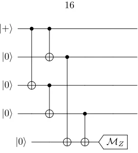
2 |00. . .0i+|11. . .1i (1.48) is prepared for each syndrome operation, using a circuit similar to Figure 1.2 where the length of the cat state is equal to the weight of the stabilizer being measured. The cat state can be tested to verify that it has been prepared correctly; if not, we throw it away and try again. After preparing a verified cat state, we can apply either a CNOT (forZ stabilizers) or a CZ gate (forX stabilizers) from separate qubits of the the cat state to the nontrivial qubits of the stabilizer being measured. Then the stabilizer can be obtained by measuring the cat state in the X basis; the parity of the physical measurement outcomes is the stabilizer measurement outcome. This measurement should be repeated to ensure fault tolerance.

(29)

|+_i _• _•

|0i •

|0_i _•

|0i MZ

1

Figure 1.2: Preparation of a verified 4-qubit cat state.

• MX

PL |+i

MX

PL |0i

• MZ

MX • MZ

[image:29.612.235.376.76.232.2]

1 Figure 1.3: Steane error correction.

A third alternative is Knill style teleported error correction [38]. This approach uses a quantum teleportation circuit [39]. E↵ectively, errors are corrected by teleporting a state with errors onto a fresh ancilla qubit. Teleported error correction will be discussed in more detail in Section 3.5.6, where a variant of the approach is used extensively.

(30)

Chapter 2

Protected Gates for

Superconducting Qubits

Ecce ancilla Domini.

–Luke 1:38

This chapter is based on work that was published in [1].

2.1 Introduction

Building a scalable quantum computer is a formidable challenge because quantum systems decohere readily and because their interactions are hard to control accurately, yet we hope to succeed some-day by prudently applying the principles of quantum error correction and fault-tolerant quantum computing. In the standard “software” approach to quantum fault-tolerance [29], the deficiencies of noisy quantum hardware (if nottoonoisy) are overcome through clever circuit design, while in the alternative “topological” approach [21], the hardware itself is intrinsically resistant to decoherence. Both approaches exploit the idea that logical qubits can be stored and processed reliably when suitably encoded in a quantum system with many degrees of freedom; perhaps both approaches will be employed together in future quantum computing systems.

(31)

use superconducting circuits for this purpose. Specifically, several authors [40–42] have proposed designs for a superconducting “0-⇡ qubit,” a circuit containing Josephson junctions. The circuit’s energy is a function of the superconducting phase di↵erence✓between the two leads of the circuit, and there are two nearly degenerate ground states, localized near ✓ = 0 and ✓ = ⇡ respectively. The splitting of this degeneracy is exponentially small as a function of extensive system parameters, and stable with respect to weak local perturbations. Thus the 0-⇡qubit should be highly resistant to decoherence arising from local noise.

For reliable quantum computing we need not just very stable qubits, but also the ability to apply very accurate nontrivial quantum gates to the qubits. A method for achieving protected single-qubit and two-single-qubit phase gates acting on 0-⇡qubits, exploiting the error-correcting properties of a continuous-variable quantum code [43], was suggested in [42], and it was claimed that the gate errors can be exponentially small as a function of extensive system parameters. In this chapter we further develop and explore the ideas behind this protected gate.

Protected phase gates are executed by turning on and o↵a tunable Josephson coupling between anLC oscillator and a qubit or pair of qubits. Assuming the qubits are perfect, we show, using analytic arguments validated by numerical simulations, that the gate errors are exponentially small when the oscillator’s impedancepL/C is large compared to~/4e2_⇡₁ _k_⌦_{, where}_L_{is the}

(32)

scheme for universal fault-tolerant quantum computation by augmenting the protected phase gates with measurements and unprotected noisy phase gates. Section 2.13 contains our conclusions, and some further details are contained in Appendices.

2.2 The 0-⇡

qubit

For most of this chapter we will be concerned with the dynamics of gates built from the 0-⇡qubit, and will treat the qubit itself as a black box. In this section we will outline the ideas behind the qubit itself, which was proposed in [42].









_

_



_

Figure 2.1: The energyE(✓) of the 0-⇡qubit. The energy is a periodic function with period⇡of the phase di↵erence✓ between its two leads, aside from exponentially small corrections. The two basis states _{|0_i,_|1_i} of the qubit, localized near the minima of the energy at ✓ = 0 and ✓ = ⇡ respectively, are nearly degenerate.

(33)























_





_

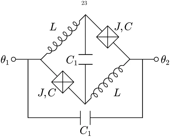
Figure 2.2: Two-rung superconducting circuit underlying the 0-⇡ qubit. If pL/C is large, C1

is large compared to C, and JC is not too large, then the circuit’s energy is a function of the combination of phases (✓2+✓4) (✓1+✓3), aside from corrections that are exponentially small in

p L/C.

at ✓ = ⇡) of an encoded qubit, as shown in Figure 2.1. The largeness of the barrier suppresses the odds of a bit flip error, and the degeneracy of the two states, enforced by the⇡ periodicity, suppresses the odds of a dephasing error. The system is designed so that this degeneracy is robust against generic local perturbations, so that the error protection is not broken.

To get such a system, we start with the four-lead circuit shown in Figure 2.2. This circuit has two identical rungs, connected by a large capacitanceC1. Each rung consists of a Josephson junction,

with Josephson energy J and intrinsic capacitance C, connected in series with an inductance L, chosen such that pL/C is large compared to the natural unit of impedance ~/(2e)2

⇡ 1.03 k⌦, and hence much larger than its “geometric” value 4⇡/c ⇡377 ⌦ (where c is the speed of light), the impedance of free space. Achieving such a “superinductance” may be a daunting experimental challenge, but we take it for granted here that it is possible. The properties of a single rung, which can operate as an adiabatic switch whenJ varies, is discussed in more detail in Appendix 2.A.

We denote the value of the superconducting phase on the circuit’s four leads as ✓1, ✓2, ✓3, ✓4

as shown, and the phase on either side of the capacitor connecting the rungs by'1, '2. Then the

phase'+= ('1+'2)/2 is insensitive to the value of the capacitanceC1, which we assume is much

larger than C. Therefore the sum'+ is a “light” variable with large fluctuations (assuming JC

is not too large), while in contrast the di↵erence' ='1 '2, which does feel the e↵ect of the

large capacitanceC1, is a well localized “heavy” variable. We assume that phase slips through the

(34)

A circuit with capacitanceCconv and inductanceLconv has Hamiltonian

H = q

2

2Cconv + 2

2Lconv, (2.1)

whereq is the charge on the capacitor and is the magnetic flux linking the circuit. We use the subscript “conv” to indicate that capacitance and inductance are expressed here in conventional units, while we will find it more convenient to use rationalized units such that

C=Cconv/(2e)2, L=Lconv/(~/2e)2, (2.2)

so that

H = Q

2

2C + '2

2L, (2.3)

where the chargeQ=q/2eis expressed in units of the Cooper pair charge 2e, and'= (2e/~) is the superconducting phase, such that '= 2⇡ corresponds to the quantumh/2e of magnetic flux. Then [', Q] =i, and

p

L/C=pLconv/Cconv/ ~/4e2

⇡pLconv/Cconv/ (1.03k⌦)

(2.4)

is dimensionless. The ground state of the Hamiltonian Equation (2.3), with energyE0= 1/2

p LC, has Gaussian wave function (') such that

| (')_|2=_p 1 ⇡h'2_ie

'2_/₂

h'2

i_, _(2.5)

where

h'2

i= 1 2

r L

C. (2.6)

(35)

cosine nearly average out, aside from an exponentially small correction:

hcos'i=p 1 ⇡_h'2_i

Z 1

1

cos'e '2/2h'2id'

=p 1 ⇡_h'2_i

Z 1

1

e '2/2h'2i+i'd' =e h'2i/2

= exp 1 4 r L C ! . (2.7)

The e↵ective capacitance controlling the light phase'+isCe↵= 2C, and the e↵ective inductance isLe↵=L/2. Therefore, in the circuit’s ground state we have

h'2+i=

1 2

r Le↵ Ce↵

=1 4

r L

C. (2.8)

The dependence of the Josephson energy on the strongly fluctuating light variable'+is proportional

to

hcos'+i= exp

1 8 r L C ! , (2.9)

which is negligible whenpL/C is large. We therefore need only consider the dynamics of the well localized heavy variable' , which locks to the value

= (✓4 ✓1) (✓3 ✓2) = (✓2+✓4) (✓1+✓3), (2.10)

determined by the phases on the leads, so that the energy stored in the circuit is

E=f(✓2+✓4 ✓1 ✓3) +O exp

1 8 r L C !! , (2.11)

wheref(✓) is a periodic function with period 2⇡.

Now, to devise a qubit, we twist the upper rung relative to the lower one and connect the leads as shown in Figure 2.3, thus identifying ✓2 with✓4 and ✓1 with ✓3. In addition, we add another

(36)



_









_









_

[image:36.612.161.457.76.311.2]



_

Figure 2.3: The circuit for the 0-⇡ qubit is obtained from the circuit in Figure 2.2 by twisting one of the rungs and connecting the leads, thus identifying✓2 with✓4and✓1 with✓3. In addition,

another large capacitance is added to further suppress tunneling events that change✓2 ✓1 by⇡.

energy of the resulting circuit is

E=f(2(✓2 ✓1)) +O exp 1

8 r

L C

!!

, (2.12)

where the ellipsis represents exponentially small corrections. Therefore, the energy is very nearly a periodic function with period⇡of the phase di↵erence✓2 ✓1, with two nearly degenerate minima

as in Figure 2.1.

2.2.1 Achieving superinductance

(37)

arises because the correction terms in Equation (2.12) that break the⇡-periodicity are associated with quantum tunneling from one end to the other in the two-rung ladder. We also require ¯JC¯ to be large, to suppress phase slips due to tunneling across the chain, thus ensuring that'+ can be

regarded as a real variable rather than a periodic variable with period 2⇡.

An impedance pL/C _⇡20 has been achieved using long chains of devices [44–46]. Another possibility for achieving large pL/C is to use a long wire, thick enough to suppress phase slips, built from an amorphous superconductor with a large kinetic inductance. Whatever method is used, reaching, say,pL/C of order 100 may be quite challenging, but in this thesis we take it for granted that a robust 0-⇡ qubit can be realized. In fact, our scheme for implementing accurate quantum gates will also be based on superinducting circuits.

2.2.2 Measurements

We will need to be able to measure the qubit, in either the standard_{|0_i,_|1_i} basis (measurement of the Pauli operatorZ) or in the dual basis_{|+_i,_| _i}(measurement of the Pauli operator X). In principle, theZ measurement could be performed by connecting the two leads of the qubit with a Josephson junction, while inserting 1/4 of a flux quantum through the loop; then the current through the junction is proportional to sin (✓2 ✓1 ⇡/2), with sign dependent on whether✓2 ✓1

is 0 or⇡.

For measuringX, we envision “breaking” the connection between✓1and✓3and then measuring

the charge conjugate to the phase di↵erence✓1 ✓3. The energy of the circuit isf(✓1+✓3 2✓2),

so that if ✓1 advances adiabatically by 2⇡ with ✓3 fixed, then ✓2 advances by ⇡; if X = 1 the

wave function is invariant and if X = 1 the wave function changes sign. Correspondingly, the dual charge is either an even or odd multiple of 1/2. In practice, the X andZ measurements are bound to be noisy, but the limitations on measurement accuracy can be overcome by repeating the measurements or by using appropriate coding schemes, as we describe in Section 2.12.

2.3 Phase gate

Following [42], we will explain how to execute with high fidelity the single-qubit phase gate exp i⇡₄Z and the two-qubit phase gate exp i⇡

4Z⌦Z . These gates are not sufficient by themselves for

(38)









[image:38.612.207.405.74.241.2]



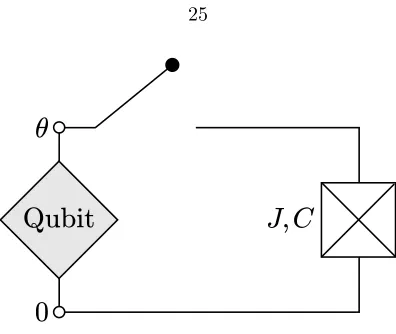
Figure 2.4: A phase gate can be applied to a qubit by coupling it to a Josephson junction, but the gate is not protected against pulse errors and other noise sources.

a universal fault-tolerant scheme.

First, for contrast, consider an example of an unprotected single-qubit gate implementation. As shown in Figure 2.4, we could close a switch that couples the qubit for timet to a Josephson junction with Josephson couplingJ, in e↵ect turning on a term Jcos✓=JZ in the Hamiltonian, where✓ ₂_{0,⇡_} is the phase di↵erence across the qubit. After timet the unitary transformation exp( itJZ) has been applied. By choosing the timetappropriately, we can rotate the qubit about thez axis by any desired angle. However, this gate is sensitive to errors in the pulse that closes and opens the switch, and to other fluctuations in the circuit parameters. For example, if we leave the gate on for too long, the accumulated error is linear in the gate mistiming.

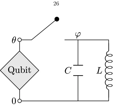
The protected single-qubit phase gate is executed as shown in Figure 2.5, by coupling the qubit to a “superinductive” LC circuit via a switch that pulses on and o↵. The switch is actually a tunable Josephson junction, which can be realized, as in Figure 2.6, by a loop containing two identical junctions, each with Josephson couplingJ, linked by the magnetic flux (⌘/2⇡) 0, where

0=h/2eis the flux quantum. The Josephson energy of this tunable junction is

E(✓,⌘) = Jcos(✓ ⌘/2) Jcos(✓+⌘/2) = 2Jcos(⌘/2) cos✓

(39)













Figure 2.5: A protected phase gate is executed by coupling a qubit (or a pair of qubits connected in series) to a “super-quantum”LC circuit withpL/C 1.



[image:39.612.208.405.75.264.2]



Figure 2.6: An e↵ective Josephson junction can be tuned by adjusting the flux (⌘/2⇡) 0 inserted

in a circuit containing two identical junctions.

(40)







_

Figure 2.7: The profile of the tunable Josephson couplingJ(t) in the execution of the protected phase gate.

2.3.1 Ideal protected phase gate

We will first describe how the protected phase gate works in the ideal case with no errors. In the following section we will discuss the e↵ects of the imperfections and argue that their e↵ects are minor.

Using the same normalization conventions as in Section 2.2, the Hamiltonian for the circuit can be expressed as

H(t) = Q

2

2C + '2

2L J(t) cos(' ✓), (2.14)

where nowJ(t) is the time-dependent e↵ective Josephson coupling of the tunable junction,✓is the phase di↵erence across the qubit, and ' is the phase di↵erence across the inductor. We assume that phase slips through the circuit are strongly suppressed, so that' can be regarded as a real variable rather than a periodic phase variable — when'winds by 2⇡the flux linking theLCcircuit increases by one flux quantum. Depending on whether the state of the qubit is|0ior|1i, the phase ✓is either 0 or⇡; hence, the Hamiltonian can be expressed as

H0,1(t) =

Q2

2C + '2

2L⌥J(t) cos', (2.15)

with the_⌥sign conditioned on the qubit’s state. Suppose the initial state _| in

(41)



_



   













_



 

  







[image:41.612.210.405.75.384.2]



Figure 2.8: Coupling the qubit to the oscillator prepares a grid state in'space, a superposition of narrowly peaked functions governed by a broad envelope function. The peaks occur where'is an even multiple of⇡if the qubit’s state is_|0_i, and where 'is an odd multiple of⇡if the qubit’s state is_|1_i.

the constant valueJ0. We assume that J(t) ramps up slowly enough to prepare adiabatically the

ground state in each local minimum of the cosine potential, yet quickly enough to prevent the state from collapsing to just a few local minima with the smallest values of'2_{/2L. Thus, as}_J_{(t) turns}

on, the initial state of the oscillator evolves to become a “grid state,” as shown in Figure 2.8, a superposition of narrowly peaked functions governed by a broad envelope function. The width of the broad envelope is_h'2

i ⇡ 1 2

p

L/C 1, as for the oscillator’s initial state, while the width of each narrow peak is _h(' '0)2i ⇡ 1₂

p

1/J0C ⌧1, the width of the ground state supported near

the local minimum of the cosine potential.

(42)

then the narrow peaks occur where' is an even multiple of ⇡. We denote this grid state of the oscillator as_|0Ci; the subscript stands for “code,” since, as we will explain later, this state can be

regarded as a basis state for a quantum error-correcting code. If the state of the qubit is_|1_iand the coefficient of the cosine is positive, then the narrow peaks occur where'is an odd multiple of⇡; in that case we denote the grid state as_|1Ci. Thus, if the initial state of the 0-⇡qubit isa|0i+b|1i,

then whenJ(t) turns on, the joint state of the qubit and oscillator evolves according to

(a_|0_i+b_|1_i)_| in_{i !}a_|0_{i ⌦}_|0Ci+b|1i ⌦|1Ci. (2.16)

After the Gaussian grid state has been prepared, the Josephson coupling J(t) maintains its steady-state valueJ0for a timet⌘L˜t/⇡, where ˜tis a rescaled time variable. While the coupling is

on, each narrowly peaked function is stabilized by the strongly confining cosine potential, but the state is subjected to the Gaussian operatione it'2_/₂_L

=e i˜t'2_/_2⇡

, due to the harmonic potential '2_{/2L, which alters the relative phases of the peaks. As ˜}_t _{increases the oscillator states}

|0Ciand

|1Ci evolve, but when ˜t reaches 1, each returns to its initial value, apart from a state-dependent

geometric phase. For the grid state |0Ci, the peaks in ' space occur at '= 2⇡n, where n is an

integer, and the Gaussian operation

|'= 2⇡n_{i !}e 2⇡itn˜2_|'= 2⇡n_i =e 2⇡in2

|'= 2⇡n_i

=|'= 2⇡ni (2.17)

acts trivially. But for the grid state_|1Ci, the peaks occur at'= 2⇡(n+1₂), and the operation

|'= 2⇡n_{i !}e 2⇡i˜t

⇣

n+1₂⌘2

|'= 2⇡(n+1 2)i

=e 2⇡i

⇣

n2₊_n₊1 4 ⌘

|'= 2⇡(n+1 2)i

=e i⇡2|_'_{= 2⇡(n}₊1

2)i (2.18)

(43)

oscillator becomes

a|0i ⌦|0Ci+b|1i ⌦|1Ci !a|0i ⌦|0Ci ib|1i ⌦|1Ci. (2.19)

To complete the execution of the phase gate, the tunable couplingJ(t) ramps down fromJ0 to

zero, again with a characteristic time scale ⌧J subject to the constraints specified above. As the

coupling turns o↵, the state |0Ci of the oscillator evolves to | fin0 i and the state |1Ci evolves to

| fin

1 i; the final joint state of the qubit and oscillator is

a_|0_{i ⌦}_|0Ci ib|1i ⌦|1Ci !a|0i ⌦| 0fini ib|1i ⌦| 1fini. (2.20)

Thus, a perfect phase gate exp i⇡

4Z has been applied to the qubit if| fin

0 i=| fin1 i. If, on the other

hand,_|h fin

1 | 0fini|<1, then the qubit and oscillator are entangled in the final state, compromising

the gate fidelity. Even if_|h fin

1 | 0fini|= 1 so that there is no entanglement, the gate may be imperfect

because the phase of_h fin

1 | 0finideviates from zero.

The two-qubit phase gate exp(i⇡₄Z ⌦Z) is executed using a similar procedure, but now two qubits connected in series are coupled to the LC oscillator. The total phase di↵erence across the pair of qubits is either 0 for the states|0i ⌦|0iand|1i ⌦|1i, in which case the oscillator evolves to the final| fin

0 i, or⇡for the states|0i ⌦|1iand|1i ⌦|0i, in which case the oscillator evolves to the

final state_| fin

1 i. Again, the gate is executed perfectly if| fin0 i=| 1fini.

2.3.2 E

↵

ects of protected phase gate imperfections

Suppose for now that the initial state _| in

i of the oscillator is its ground state, a Gaussian wave function with_h'2

i= 1 2

p

L/C and_hQ2

i= 1 2

p

C/L. (Other harmonic oscillator energy eigenstates will be considered in Section 2.10.) BecausepL/C 1, the wave function is broad in'space and narrow in Qspace. Hence, when the switch pulses on, the contribution to the expectation of the energy arising from the cosine potential is highly suppressed by the factor

hcos'i=e h'2i/2= exp 1 4

r L C

!

(44)

as derived in Equation (2.7). Correspondingly, the energy is very insensitive to the state of the qubit, which determines the sign of the cosine potential. This suppression factor determines the characteristic scale of the error in the phase gate.

As we turn on the Josephson couplingJ(t) with the form shown in Figure 2.7, the characteristic time⌧J for the coupling to ramp on and o↵ is subject to some constraints, which we will specify

shortly. WithJ at its steady state valueJ0, phase slips (tunneling events between successive minima

of the cosine potential) are suppressed by the WKB factor

exp

✓ Z 2⇡

0

d'p2J0C(1 cos')

◆

= exp( 8pJ0C). (2.22)

We assume thatpJ0C is large enough so that phase slips can be safely neglected.

A diabatic transition that excites the oscillator in the cosine well is most likely to occur while J(t)C is approximately one and the frequency of oscillations in the well is approximately 1/C. We will pass through this regime once when ramping up the gate and once again ramping down. Landau-Zener theory indicates that the probabilityPdiabof such a transition scales like

Pdiab(⌧J)⇠exp

⇣

(constant)⌧J C ⌘

, (2.23)

where⌧J is the characteristic time forJ(t) to ramp on. (We will discuss this error in more detail

in Section 2.7.) Since diabatic e↵ects also contribute to the error in the phase gate, we require ⌧J C. Indeed, the diabatic error is comparable to the intrinsic error in Equation (2.21) for

⌧J⇠

p

LC; (2.24)

that is, when the ramping time is on the order of the period of the LC oscillator. During this ramping time, the envelope function of the Gaussian grid state is squeezed somewhat in 'space (and correspondingly spreads somewhat inQspace), but stays broad enough for the intrinsic error to remain heavily suppressed. In Section 2.8 we argue that the error arising from squeezing scales like

Psq(⌧J)⇠exp

✓

(constant)L ⌧J

◆

; (2.25)

(45)

We will argue that under appropriate conditions_h fin

1 | 0fini ⇡1 to extremely high accuracy so

that the phase gate is nearly perfect. Note that we need not require the final state of the oscillator to match the initial state_| in

i; noise terms in the Hamiltonian may excite the oscillator, but the phase gate is still highly reliable as long as the oscillator’s final state depends only very weakly on the state of the 0-⇡qubit,i.e., on whether the sign ofJ(t) is positive or negative. Indeed, the oscillator serves as a reservoir that absorbs the entropy introduced by noise. If not too badly damaged, the oscillator can be reused a few times for the execution of additional protected gates. Eventually, though, it will become too highly excited, and will need to be cooled before being employed again. A gate error may arise if the coupling between qubit and oscillator remains on for too long or too short a time, i.e., if ˜t = 1 +" rather than ˜t = 1. But we will see that such timing errors do not much compromise the performance of the gate when" is small; specifically, the gate error is exp⇣ 1

4

p

L/C⌘_⇥O(1) provided _|"_| < 2⇡(L/C) 3/4. Slightly overrotating or underrotating contributes to the damage su↵ered by the oscillator, but without much enhancing the sensitivity of the oscillator’s final state to the qubit’s state, and hence without much reducing the fidelity of the gate. We study the consequences of overrotation/underrotation in Section 2.6, and we confirm our findings using numerical simulations in Section 2.9. We also argue, in Sections 2.10 and 2.11, that the phase gate is robust against a sufficiently small nonzero temperature and against small perturbations in the Hamiltonian.

Let us summarize the sufficient conditions for the phase gate to be well protected. Just as for the realization of the 0-⇡ qubit itself, the execution of the protected phase gate relies on the construction of a “superinducting” circuit with pL/C 1. This is a daunting experimental challenge, as we have already noted at the end of Section 2.2. To ensure high gate accuracy, we also assume that the steady state valueJ0of the Josephson coupling between the 0-⇡qubit and the

oscillator satisfiespJ0C 1, and that the characteristic time scale⌧J for the coupling to ramp

on and o↵isO(pLC); thus⌧J is also small compared to the timeL/⇡needed to execute the gate.

(46)

2.4 Sketch of the error estimate

A noisy quantum gate realizes a quantum operation_Nactual, and a useful way to quantify the error

in the gate is to specify the deviation_kNactual Nidealk_⌃from the ideal gateNidealin the “diamond

norm” [6]. As explained in Appendix 2.B, for the protected phase gate this diamond norm distance (assuming there are no bit flips) is

kNactual Nidealk_⌃=|1 h 1fin|,i 0fin| (2.26)

where_| fin

0,1idenotes the final state of the oscillator when|0i,|1iis the state of the 0-⇡qubit, as in

Equation (2.20). Thus, we assess the gate accuracy by estimating the deviation of_h fin

0 | 1finifrom

1.

To perform this estimate we track how the oscillator states_| 0(t)iand| 1(t)iare related through

three stages of evolution:

| in

i J(t) turns on!| 0begini

J(t)=J0

! | end

0 i

J(t) turns o↵ !| fin

0 i,

| ini J(t) turns on!| 1begini

J(t)=J0

! i_| 1endi

J(t) turns o↵

! i_| 1fini.

(2.27)

In the first stage J(t) ramps on and the grid states are prepared – the initial state _| in

begin

1 i evolves

to i_| end

1 i, where ideally| end0,1i=| begin

0,1 i. In the third stageJ(t) ramps o↵and the grid states

| end

0,1ievolve to the final oscillator states| fin0,1i, where ideally| fin1 i=| fin0 i.

Consider the first (or third) stage of the evolution, where the couplingJ(t) ramps on (or o↵) in a time of order⌧J. If⌧J is not too large compared to the period 2⇡pLC of the oscillator, then the

harmonic potential term'2_/2L_{may be treated perturbatively during this evolution stage. Hence,}

in first approximation the Hamiltonian is one of

H0=

Q2

2C J(t) cos', H1= Q2

(47)

simultaneously diagonalized. We may express the eigenvalue of this translation operator ase 2⇡iq_,

whereq=Q [Q]₂[ 1 2,

1

2] is the conserved Bloch momentum, and [Q] denotes the nearest integer

toQ; thus [Q] labels the distinct bands in the Hamiltonian’s spectrum.

A diabatic transition between bands may be excited whileJ(t) varies, changing the value of [Q] by an integer, most likely_±1. If such transitions occur with nonnegligible probability, the final state of the oscillator will contain, in addition to a primary peak supported nearQ= 0, also secondary peaks supported nearQ=±1; the phases of the secondary peaks depend on whether the Hamilto-nian isH0 or H1, and therefore diabatic transitions contribute to the gate error. The probability

of a diabatic transition cannot be computed precisely, but, as we will explain in Section 2.7, it can be analyzed semi-quantitatively, and is very small if⌧J is sufficiently large.

For the purpose of discussing this diabatic error and other contributions to the deviation of h fin

1 | fin0 ifrom 1, we will find it useful to consider the operator

¯

X ⌘( 1)[Q] =⇧Qeven ⇧

Q

odd

= 2⇧Qeven I=I 2⇧

Q

odd.

(2.29)

Here ⇧Q

even projects onto values of Q such that the nearest integer value [Q] is even and ⇧Qodd

projects onto values ofQ such that [Q] is odd. We denote this operator as ¯X because it can be regarded as the error-corrected Pauli operator X _{acting on a qubit encoded in the Hilbert space}

of the oscillator, as we explain in Section 2.5. (Note that ¯X2 ₌_{I.) Another (related) important}

property is that, sincee⌥i'_translates_Q_by

±1, ¯X anticommutes with cos':

¯

Xcos'X¯ = cos'. (2.30)

Our argument showing that | fin

1 i ⇡ | 0fini has two main elements. On the one hand, we use

approximate symmetries and properties of grid states to see that_| 1(t)i ⇡X¯| 0(t)iat each stage

of the oscillator’s evolution, so that in particular _| fin

1 i ⇡X¯| fin0 i. On the other hand, we argue

that if the time scale ⌧J for J(t) to turn on and o↵is suitably chosen, then the oscillator’s final

state is mostly supported nearQ= 0, so that in particular ¯X_| fin

0 i ⇡| fin0 i.

We note that the approximate HamiltoniansH0and H1 in Equation (2.28) are related by

(48)

By integrating the Schr¨odinger equation using the HamiltonianH0or H1 during the first stage of

evolution while J(t) ramps on, we obtain the unitary time evolution operatorsU0, U1, which are

related by

U1= ¯XU0X.¯ (2.32)

Thus, the initial oscillator state_| in

ievolves to one of the states

| begin0 i=U0| ini

| begin1 i=U1| ini= ¯XU0X¯| ini,

(2.33)

and therefore

h 1begin|X¯| begin

0 i=h in|X¯| ini

=_h in_|I 2⇧Q_odd_| in_i

= 1 2h in

|⇧Q_odd| in

i. (2.34)

We conclude that if the initial state is almost fully supported on even values of [Q] (for example, the oscillator ground state, a Gaussian inQ-space with width much less than 1/2), then| 1beginiis

very close to ¯X| 0begini.

So far, we have ignored the e↵ects of the quadratic term '2_/2L _{in the potential. This term}

can cause the wave function to broaden in Q-space and be squeezed in ' space, but we argue in Section 2.8 that this squeezing is a relatively small e↵ect, so that the conclusion _| ₁begin_{i ⇡}

¯

X_| ₀begin_i still holds accurately. Specifically, the contribution to the gate error due to squeezing scales according to Equation (2.25), and hence becomes comparable to the other sources of error when we choose⌧J⇠

p LC.

During the second stage of the evolution, whileJ(t) =J0is held constant, distinct peaks in the

grid state acquire relative phases, and the condition_| 1(t)i = ¯X| 0(t)ibecomes badly violated.

However, after a timet⇡L/⇡, the initial states| 0beginiand| begin

1 iare restored, aside from the

state dependent phase i, and hence| end

1 i= ¯X| end0 i, apart from a small error. Equivalently, the

beginning states

| ±begini= 1 p 2

⇣

| 0begini± | begin

1 i

⌘

Quantum Error Correction with Biased Noise