Mostly harmless simulations? Using Monte Carlo studies for estimator selection

(1)

Manuscript version: Working paper (or pre-print)

The version presented here is a Working Paper (or ‘pre-print’) that may be later published elsewhere.

Persistent WRAP URL:

http://wrap.warwick.ac.uk/116252

How to cite:

Please refer to the repository item page, detailed above, for the most recent bibliographic citation information. If a published version is known of, the repository item page linked to above, will contain details on accessing it.

Copyright and reuse:

The Warwick Research Archive Portal (WRAP) makes this work by researchers of the University of Warwick available open access under the following conditions.

Copyright © and all moral rights to the version of the paper presented here belong to the individual author(s) and/or other copyright owners. To the extent reasonable and practicable the material made available in WRAP has been checked for eligibility before being made available.

Copies of full items can be used for personal research or study, educational, or not-for-profit purposes without prior permission or charge. Provided that the authors, title and full

bibliographic details are credited, a hyperlink and/or URL is given for the original metadata page and the content is not changed in any way.

Publisher’s statement:

Please refer to the repository item page, publisher’s statement section, for further information.

(2)

Warwick Economics Research Papers

ISSN 2059-4283 (online)

Mostly Harmless Simulations? Using Monte Carlo Studies

for Estimator Selection

Arun Advani, Toru Kitagawa and Tymon Słoczyński

(This paper also appears as CAGE Working paper 411)

(3)

M

OSTLY

H

ARMLESS

S

IMULATIONS

?

U

SING

M

ONTE

C

ARLO

S

TUDIES FOR

E

STIMATOR

S

ELECTION

∗

A

RUN

A

DVANI

,

†

T

ORU

K

ITAGAWA

,

‡ AND

T

YMON

S

ŁOCZYNSKI

´

§

Summary

We consider two recent suggestions for how to perform an empirically mo-tivated Monte Carlo study to help select a treatment effect estimator under unconfoundedness. We show theoretically that neither is likely to be infor-mative except under restrictive conditions that are unlikely to be satisfied in many contexts. To test empirical relevance, we also apply the approaches to a real-world setting where estimator performance is known. Both approaches are worse than random at selecting estimators which minimise absolute bias. They are better when selecting estimators that minimise mean squared error. However, using a simple bootstrap is at least as good and often better. For now researchers would be best advised to use a range of estimators and compare estimates for robustness.

JEL Classification: C15, C21, C25, C52

Keywords: empirical Monte Carlo studies, program evaluation, selection on observables, treatment effects

∗_{This version: March 21, 2019. Previously circulated as ‘Mostly Harmless Simulations? On the}

Inter-nal Validity of Empirical Monte Carlo Studies’. For helpful comments, we thank Thierry Magnac (Co-Editor), four anonymous referees, Alberto Abadie, Cathy Balfe, Richard Blundell, Colin Cameron, M ´onica Costa Dias, Gil Epstein, Alfonso Flores-Lagunes, Ira Gang, Martin Huber, Justin McCrary, Blaise Melly, Ma-teusz My´sliwski, Pedro Sant’Anna, Tony Strittmatter, Tim Vogelsang, Ed Vytlacil, Jeff Wooldridge, Tiemen Woutersen, and numerous seminar and conference participants. We also thank Michael Lechner and Blaise Melly for providing us with their codes, as well as Steven Karel and Francesco Pontiggia for assistance with the Brandeis HPC cluster. This research was supported by a grant from the CERGE-EI Foundation under a program of the Global Development Network (Grant No: RRC12+09). All opinions expressed are those of the authors and have not been endorsed by CERGE-EI or the GDN. Advani also acknowledges sup-port from Programme Evaluation for Policy Analysis, a node of the National Centre for Research Methods, supported by the ESRC (Grant No: RES-576-25-0042). Kitagawa also acknowledges support from the ESRC through the ESRC Centre for Microdata Methods and Practice (cemmap) (Grant No: RES-589-28-0001) and from the ERC through an ERC starting grant (Grant No: EPP-715940). Słoczy ´nski also acknowledges sup-port from the Foundation for Polish Science (FNP) through a START scholarship and from the Theodore and Jane Norman Fund. No authors are aware of any conflict of interest.

†_{University of Warwick, CAGE, and Institute for Fiscal Studies.} ‡_{University College London and cemmap.}

§_{Brandeis University and IZA. Correspondence: Department of Economics & International Business}

(4)

1 Introduction

A large literature focuses on estimating average treatment effects under

unconfounded-ness (see, e.g., Blundell and Costa Dias 2009, Imbens and Wooldridge 2009, Abadie and

Cattaneo 2018).1 Many estimators are available to researchers in this context, and many

of these estimators have similar asymptotic properties. This can make it difficult to select which estimator to use. Monte Carlo studies are a useful tool for examining the

small-sample properties of these estimation methods, which can guide estimator choice.2 Early

contributions, such as Fr ¨olich (2004), demonstrate estimator performance in stylised data generating processes (DGPs) which do not resemble any empirical settings. This reliance

on unrealistic DGPs is criticised by Huber et al.(2013) and Busso et al. (2014). Both

rec-ommend that Monte Carlo studies should intend to replicate actual datasets of interest,

although they suggest different procedures for doing this. Huberet al.(2013) describe this

approach to examining the small-sample properties of estimators as an ‘empirical Monte Carlo study’ (EMCS). An important question is whether either type of EMCS can help

applied researchers in choosing what estimator(s) to prefer in a given context. Bussoet al.

(2014) indicate this might be possible, noting that their results ‘suggest the wisdom of conducting a small-scale simulation study tailored to the features of the data at hand’.

Similarly, Huberet al.(2013) suggest that ‘the advantage [of an EMCS] is that it is valid in

at least one relevant environment’,i.e.that it is informative at least about the performance

of estimators in the dataset on which it was conducted.

In this paper we evaluate the premise that EMCS can be informative about the per-formance of estimators in the particular data which are the basis for the EMCS. We first show theoretically that these approaches are expected to be informative only under very restrictive conditions. These conditions are unlikely to hold in many practical examples faced by a researcher. We then test EMCS performance in a real-world case where we know the actual behaviour of estimators. We find that in terms of selecting estimators on absolute bias they are often worse than choosing randomly. On mean squared error (MSE) they perform better than random, but no better than selecting an estimator based on simple bootstrap estimates of MSEs. Their performance in absolute terms may also still be poor.

1_{The unconfoundedness assumption may also be referred to as exogeneity, ignorability, or selection on}

observables.

2_{See, for example, Fr ¨olich (2004), Lunceford and Davidian (2004), Zhao (2004, 2008), Busso}_{et al.}_(2009),

(5)

The first type of EMCS we consider is the placebo EMCS (Huber et al., 2013).3 This proposes a way to assign ‘realistic placebo treatments among the non-treated’, using in-formation about the predictors of treatment status in the original data. It then tests how well estimators can recover the zero effect of the placebo treatment. The performance of estimators in this exercise is hypothesised to be informative about their performance in the original data.

The second type we describe as the structuredEMCS. An exercise of this type is

un-dertaken by Bussoet al.(2014).4 Here a parameterised approximation of the original data

generating process is created, using functional form assumptions about the distributions of observed covariates. Parameters of their marginal (or conditional) distributions are estimated from the original data. Samples can be drawn from this approximate DGP, to which the estimators can then be applied. Since the treatment effect in this DGP can be calculated directly from knowledge of the parameters, performance of the estimators in these samples can be measured. The performance of estimators in this exercise is also hypothesised to be informative about their performance in the original data.

To examine whether or not EMCS can correctly choose a best performing estimator, for various definitions of performance, we first focus on a simple example with two esti-mators that have Gaussian sampling distributions. We show analytically that both these approaches will only be guaranteed to correctly select the preferred estimator if they can correctly reproduce both the biases and the ordering of the variances of estimators. These are restrictive conditions that we show can easily fail in practical applications, such as when the EMCS procedures fail to recover heteroskedastic errors or misspecify the re-gression equations or propensity scores. In two sets of simulations based on a stylised DGP, both approaches select the better estimator less than 3% of the time, much worse than 50% achievable by selecting randomly.

To study the extent of the problem in a real-world circumstance, we apply both meth-ods to the National Supported Work (NSW) Demonstration data on men, previously anal-ysed by LaLonde (1986), Heckman and Hotz (1989), Dehejia and Wahba (1999, 2002), Smith and Todd (2001, 2005), and many others. In these data participation in a job train-ing programme was randomly assigned, so the treatment effect of the programme can be estimated by comparing sample means. LaLonde (1986) used these data to test the performance of estimators at reproducing this treatment effect when an artificial compar-ison group (rather than the experimental controls) was used. We instead use the data to

3_{It is also applied by Lechner and Wunsch (2013), Huber}_{et al.}_{(2016), Fr ¨olich}_{et al.}_{(2017), Lechner and}

Strittmatter (2017), and Bodoryet al.(2018). A related approach is proposed by Schuleret al.(2017).

(6)

test how well the two EMCS procedures can inform us about the performance of the es-timators: Can EMCS tell us which estimator to use? On average how much worse than the optimal estimator is the one chosen by EMCS? How well can EMCS reproduce the ranking of performance across all estimators?

Applying the two EMCS procedures we find three main results. First, in terms of ab-solute bias, the EMCS procedures are no better, and often noticeably worse, than selecting an estimator at random. In two out of three cases we study, the rankings produced are negativelycorrelated with the true ranking. In one case the preferred estimator selected by EMCS is on average 30–37 times worse than the actual best estimator.

Second, EMCS does better at reproducing the performance of estimators in terms of MSE. This is because the MSEs of the estimators are mostly driven by their variances, and EMCS appears more effective at capturing variances. The rankings of estimators are consistently positively correlated with the true rankings, although the estimator preferred by EMCS has an MSE up to twice as high as the best estimator.

Third, given the variance result, we also compare EMCS procedures to choosing esti-mators based on performance criteria estimated from a simple nonparametric bootstrap. We find that the bootstrap is as good, and often much better, than either of the EMCS procedures. Hence even when the procedures are somewhat informative, they are not superior to a procedure that relies on fewer design choices.

These results are unfortunate, but nevertheless important. They caution against treat-ing either of these approaches as general solutions to the problem of estimator choice. There remains no silver bullet that can assist empirical researchers with the ‘right’ or ‘best’ estimator for a particular context. In the absence of a clear choice driven by research de-sign, the best advice at this stage is likely to be implementing a number of estimators, and

then considering the range of estimates provided, as Bussoet al.(2014) also suggest.

Our results also have implications for researchers studying the small-sample proper-ties of treatment effect estimators (see footnote 2). It has been argued that ‘it is preferable

to study DGPs that are empirically relevant’ (Bussoet al., 2014). Our theoretical and

em-pirical results suggest there is little support for this claim. We show theoretically that misspecification in the construction of the DGP can lead the ranking of estimators to be incorrect for the original dataset. In our empirical example, we see that EMCS is not better than using a bootstrap (and sometimes not better than random) to predict performance in the data on which the EMCS was performed. There seems to be little reason to then think

it is particularly informative about performance in other unrelated real datasets,i.e.that

(7)

performance to parameters of the simulation, such as sample size and the degree of

het-eroskedasticity. This approach is also taken by Huber et al. (2013), and might be more

helpful in understanding what characteristics of samples most affect the performance of particular estimators.

2 EMCS Designs

We first describe the two main approaches to conducting an EMCS, namely the placebo

design of Huber et al. (2013) and the structured design of Busso et al. (2014). In either

EMCS design, one simulates many ‘empirical Monte Carlo’ replication samples from a known data generating process. By implementing the estimators on the simulated repli-cations, one obtains estimates of the sampling distributions and performance criteria

(e.g., MSEs) of the estimators, according to which one ranks the candidate estimators.

Note that the researcher needs to make a choice of what criteria to use to rank estimators.

2.1 The Placebo Design

The idea of the placebo design is to assign placebo treatments to some control observa-tions, so that by construction the treatment effect is zero, and to then attempt to recover

this effect.5 In particular, covariates and outcomes(Xi,Yi)are first drawn jointly by

sam-pling (with replacement) from the empirical distribution of control observations. Using

the original dataset, the propensity score is estimated (e.g., using a logit model). The

es-timated parameters of this model φˆ are then used to assign placebo treatments to the

generated sample in the following way:

Di = 1[Si >0], (1)

Si = π+λXiφˆ +ei, (2)

whereeiis an iid error, and bothπ andλare additional parameters to be selected. While

π shifts the proportion of observations that are treated,λcontrols the extent of selection:

with λ = 1 selection on observables takes the same form in the Monte Carlo samples as

in the original dataset.

5_{A similar approach is developed by Bertrand} _{et al.} _{(2004) who study inference in}

(8)

2.2 The Structured Design

The idea of the structured design is instead to create a parameterised approximation to the original (unknown) data generating process, and then draw samples from the approx-imated process. To begin, a fixed number of treated and control observations are created, to match the number of each in the original dataset. Covariates and outcome variables are then drawn from parameterised distributions where the parameters are estimated from

the original dataset. For example, the variable blackmight come from a Bernoulli with

mean estimated from the data, and the variableearningsfrom a log-normal distribution

with mean and variance estimated from the data. The parameters of these distributions are typically estimated conditional on treatment status. Parameters of some distributions

might also be conditional on the value of other variables; e.g., earnings might be

condi-tional on race as well as treatment status. More conditioning will improve the match of the joint distribution of simulated data to the joint distribution of the original data, but will increase the number of parameters that need to be estimated.

3 Theory

To understand the conditions under which an EMCS might be informative about the pre-ferred estimator in some particular dataset, we first construct a simple example. Here we have only two estimators, with a straightforward and restricted joint sampling dis-tribution (bivariate Gaussian). This bivariate Gaussian setting mimics an ideal situation in which the finite sample distribution of the estimators is well approximated by their asymptotic distribution. We show that even in such an ideal, large sample situation, EMCS can fail to select the best estimator if the bias in any one of the estimators or the ranking of variances is not correctly replicated in the simulated samples. We provide simple common cases for treatment effect estimation in which failure to capture the biases and heteroskedasticity contaminates EMCS, and provide results from a simple simulation illustrating this. We then extend the example to the case of more than two estimators.

3.1 Simple Example: Two Estimator Case

Suppose the researcher wants to rank two estimators ˆθ1and ˆθ2according to their statistical

performances under repeated sampling. These estimators are estimating the same object

(9)

assume that the joint sampling distribution of the two estimators is bivariate Gaussian: ˆ θ1 ˆ θ2 ! ∼ N θ1 θ2 !

,Σn

!

, (3)

whereΣn = n−1Σ,Σ =

σ₁2 σ12

σ12 σ22

!

, andnis the sample size. Here, our implicit

assump-tion is that the estimators(θˆ1, ˆθ2)converge to(θ1,θ2)at

√

n-rate. Letθ0be the true value

of the parameter of interest. We allow ˆθ1 and/or ˆθ2 to be biased so thatθ1 and/orθ2 can

differ fromθ0.

We rank these estimators according to their statistical performances. Given that we often assess the performance of an estimator by its mean squared error (MSE) or mean absolute error (MAE), we may, for instance, rank the estimators according to their MSEs

or MAEs.6 Given the Gaussian assumption, the MSE of each estimator, j=1, 2, is

MSE(θˆj) = (θj−θ0)2+n−1σ_j2.

We denote by j0 ∈ {1, 2} the index of the strictly preferred estimator, assuming it

exists. Ranking the estimators is difficult in practice since we do not know the mean and

variances of the estimators as well as the true value ofθ. Proposals of the EMCS literature

aim to infer a best performing estimator j0 by estimating the sampling distribution of

ˆ

θ1 and ˆθ2 via some Monte Carlo studies. For simplicity, we assume that the estimators

simulated in EMCS also follow bivariate Gaussian,

ˆ

θ₁∗

ˆ

θ₂∗ ! ∼ N ˜ θ1 ˜ θ2 !

, ˜Σn

!

, (4)

where ˜Σn =a−n1Σ˜, ˜Σ =

˜

σ₁2 σ˜12

˜

σ12 σ˜₂2 !

, andanis the size of a simulated sample that may

dif-fer from the size of the original samplen. The underlying parameters in EMCS,(θ˜1, ˜θ2, ˜Σ),

generally depend on the original sample, but we assume for simplicity that the

depen-dence is negligible and they can be treated as constants. EMCS computes ˆθ∗₁ and ˆθ₂∗

re-peatedly using simulated samples of size an drawn from a data generating process with

6_{MSE and MAE criteria do not take into account the dependence of the estimators. One way to rank}

the estimators that takes into account their dependence is based onthe probability of being closer to the truth, Pr(|eˆ1| ≤ |eˆ2|), where ˆe1=θˆ1−θ0and ˆe2=θˆ2−θ0are the estimation errors of the two estimators. That is,

ˆ

θ1is preferred to ˆθ2if Pr(|eˆ1| ≤ |eˆ2|) >1/2 and ˆθ2is preferred to ˆθ1if Pr(|eˆ1| ≤ |eˆ2|)<1/2. Considering

(10)

the parameter value set at known value ˜θ0. For instance, the placebo EMCS approach of

Huber et al.(2013) sets ˜θ0 = 0 andan ≤ n0, the size of the control group in the original

data. The approach of structured EMCS sets ˜θ0 at an estimate ofθ0constructed from the

original sample. In implementing EMCS, we do not have to know the mean and variance

parameters of (θˆ₁∗, ˆθ₂∗), and they can be estimated with arbitrary accuracy based on the

simulated estimators. EMCS accordingly obtains the MSE of each estimator, j=1, 2, by

[

MSE(θˆj) = (θ˜j−θ˜0)2+a−n1σ˜j2.

We denote by ˆj0 the index for a best performing estimator estimated from EMCS,

ˆ

j0 ≡ arg minjMSE[(θˆj). To assess the validity of EMCS, we define a criterion of

EMCS-validityby the probability that ˆj0 coincides with j0, Pr(jˆ0 = j0), where the probability is

evaluated under repeated sampling of the original samples. In the examples to follow, we investigate how this criterion of EMCS-validity becomes one or zero depending on the parameter values in the bivariate Gaussian distributions of (3) and (4). We assume away the dependence of the parameters in (4) on the original sample for simplicity of illustration. In such a case the MSE estimates in EMCS and resulting selection of a best

estimator ˆj0are nonrandom when the number of Monte Carlo iterations is large enough.

The criterion of EMCS-validity in this case is either 1 or 0.

We can also consider theaverage regrettype criterion such asE(MSE(θˆ_jˆ₀)−MSE(θˆj0))≥

0 to quantify EMCS-validity. Here, the expectation concerns the sampling distribution of

EMCS’s selection of an optimal estimator ˆj0. This average regret criterion can quantify

severity of a wrong choice of the estimators in terms of how much MSE is on average sacrificed relative to the true best-performing estimator.

3.1.1 Scenario 1

Denote the biases in(θˆ1, ˆθ2)0byb= (b1,b2)0 = (θ1−θ0,θ2−θ0)0and the biases in(θˆ₁∗, ˆθ∗₂)0

by ˜b = (b˜1, ˜b2)0 = (θ˜1−θ˜0, ˜θ2−θ˜0)0. We start with a scenario in which (θˆ1, ˆθ2) are

un-biased and the distribution of (θˆ∗₁, ˆθ₂∗) well replicates the distribution of (θˆ1, ˆθ2) in the

following sense:

b=b˜ =0, Σ =Σ˜. (5)

Here, the biases and the sample-size-adjusted variances of the estimators simulated in EMCS coincide with those of the estimators in the original data generating process. Note

that the true parameter value assumed in EMCS, ˜θ0, does not have to agree with the true

(11)

In the current scenario, the ranking of the true MSEs clearly coincides with the

rank-ing of the MSE estimates in EMCS, implyrank-ing Pr(jˆ0 =j0) =1. This is a benchmark case in

which EMCS works. The next two scenarios show that once we depart from the assump-tions in (5), EMCS can be no longer valid.

3.1.2 Scenario 2

Assume that the estimators are free from biases both in the original data generating

pro-cess and EMCS,b =b˜ =0, but EMCS fails to replicate the normalised covariance matrix

of the estimators,Σ6=Σ˜. In this case, the MSE estimates in EMCS correctly rank the true

MSEs of the estimators (assuming σ₁2 6= σ₂2) if and only if the ordering of the variances

of the two estimators agrees between the original sampling process and the simulated

sampling process,i.e. (σ₁2−σ₂2)(σ˜₁2−σ˜₂2) > 0. Otherwise, EMCS reverses the ranking of

the estimators and incorrectly selects a suboptimal estimator as optimal, Pr(jˆ0 = j0) =0.

Hence, even when EMCS well replicates the biases of the estimators, it can fail to select a best performing estimator due to an incorrect variance ordering.

3.1.3 Scenario 3

In the third scenario, we assume that EMCS correctly replicates the variance ordering of the estimators, i.e. (σ₁2−σ₂2)(σ˜₁2−σ˜₂2) > 0, but fails to replicate the biases, (b1,b2) 6=

(b˜1, ˜b2). To be specific, we set(b˜1, ˜b2) = (0, 0), but (b1,b2) = (0,b2),b2 6= 0. This can

cor-respond to a situation that the estimator 1 is correctly specified and has no bias, whereas estimator 2 is misspecified and is subject to bias in the original data generating process. EMCS, however, fails to capture the misspecification bias in estimator 2.

Suppose σ₁2 > σ₂2 holds. The true MSEs are MSE(θˆ1) = n−1σ₁2and MSE(θˆ2) = b₂2+

n−1σ₂2, while the MSE estimates in EMCS are MSE[(θˆ1) = an−1σ˜12and MSE[(θˆ2) = a

−1

n σ˜22.

Since we assumed that EMCS correctly replicates the variance of the estimators, EMCS

selects j =2 as a best estimator. This selection of the estimator is indeed misleading ifb2

is far from zero, since if|b2|>

q

σ₁2−σ₂2

n , ˆθ1outperforms ˆθ2in terms of MSE.

(12)

3.2 Are Scenarios 2 and 3 Relevant in Treatment Effect Estimation?

We next provide simple but empirically relevant examples where we focus on the estima-tion of treatment effects, and show that both types of EMCS may yield misleading choices of the estimators for the reasons illustrated in Scenarios 2 and 3 above.

Data are given by a random sample of{(Yi,Di,Xi) : i=1, . . . ,n}, whereYi ∈ Ris unit

i’s observed post-treatment outcome,Di ∈ {0, 1}is her treatment status, andXi ∈ Rdxis a

vector of her pre-treatment characteristics whose support is assumed to be bounded. We

denote unit i’s potential outcomes by (Yi(1),Yi(0)). We assume the unconfoundedness

assumption,(Y(1),Y(0)) ⊥D|X, throughout. The propensity score is denoted bye(x) =

Pr(D =1|X= x).

3.2.1 An Example for Scenario 2

To keep our example as simple as possible, consider the following data generating pro-cesses:

E(Y(1)|X= x) = β0+β1+x0β2, (6) E(Y(0)|X= x) = β0+x0β2,

Var(Y(1)|X= x) = cσ_e2, Var(Y(0)|X =x) =σ_e2, c >0,

e(x) = γ0+x0γ1.

The specified mean equations for both potential outcomes imply that the conditional

av-erage treatment effects are homogeneous over observed characteristics and equal to β1.

The potential outcomes are heteroskedastic if c 6= 1. We assume a linear probability for

the propensity score in order to simplify analytical comparisons of the variances of the estimators we introduce below.

Suppose that the parameter of interest is the population average treatment effect for

the treated (ATT), θ0 = E(Y(1)−Y(0)|D = 1). Since specification (6) implies

homoge-neous conditional average treatment effects,E(Y(1)−Y(0)|X = x) = β1, the true value

of ATT isθ0= β1.

We consider two different estimators to estimate the population ATT. The first

estima-tor ˆθ1is a semiparametric estimator for ATT, which is consistent without assuming

func-tional forms for the outcome and propensity score equations, and asymptotically attains the semiparametric efficiency bound (SEB) of ATT derived by Hahn (1998). Estimators that attain this property include the inverse probability weighting (IPW) estimator with

(13)

esti-mators of Hahn (1998), covariate or propensity score matching estiesti-mators with a single covariate (Abadie and Imbens, 2006, 2016), and covariate balancing estimators of Chen et al.(2008) and Grahamet al.(2012, 2016). We can set any one of these estimators as our first estimator without affecting the analysis below.

We specify the second estimator ˆθ2as the ordinary least squares estimator ofβ1in the

following regression equation:

Yi= β0+β1Di+Xi0β2+ei, E(ei|Di,Xi) = 0. (7)

In other words, ˆθ2 = βˆ1,OLS. The specification of (6) implies that ˆθ2 is unbiased and

consistent for the population ATT,θ0. We consider a situation in which the finite sample

distribution of (θˆ1, ˆθ2) is well approximated by its large sample normal approximation,

i.e. ˆ θ1 ˆ θ2 ! ∼ N θ0 θ0 ! , 1 n

σ₁2 σ12

σ12 σ₂2 !!

,

where σ₁2 is the asymptotic variance of

√

n(θˆ1−θ0) given by SEB for ATT without the

knowledge of propensity scores, andσ₂2is the asymptotic variance of

√

n(θˆ2−θ0). Under

the current specification, they are obtained as

σ12=

σ_e2

Pr(D =1)

c+E

e(X)

1−e(X)|D =1

, (8)

σ₂2= σ

2

e

Pr(D =1)

c· E((1−e(X))

2_|_D₌₁₎

[E(1−e(X)|D=1)]2 +

E(e(X)(1−e(X))|D=1) [E(1−e(X)|D =1)]2

. (9)

See Appendix A for their derivations.

WhenY(1)andY(0) share the variance (c = 1), it can be shown that the OLS

estima-tor is more efficient than the semiparametric estimaestima-tor, σ₂2 < σ₁2, due to exploitation of

the correct functional form of the regression equation. In contrast, if the variance of the

treated outcome is higher than the variance of the control outcome (c > 1), the simple

OLS estimator that does not take into account the heteroskedastic errors can become less efficient than the semiparametric estimator. Specifically, we show in Appendix A that

σ₂2 >σ₁2 iffc > ∆1

∆2

+1, where (10)

∆1=E

1

1−e(X)|D=1

− 1

E(1−e(X)|D =1) ≥0,

∆2= E

((1−e(X))2|D=1)

(14)

Hence, if the degree of heteroskedasticity satisfies the condition in (10), the

semiparamet-ric estimator ˆθ1is strictly preferred to the OLS estimator ˆθ2.

Given thatcmeets (10), consider applying the placebo EMCS proposed in Huberet al.

(2013). We assume that the two estimators are centred at zero and their simulated distri-butions can be well approximated by bivariate Gaussian,

ˆ

θ₁∗

ˆ

θ₂∗ ! ∼ N 0 0 ! , 1 n0 ˜

σ₁2 σ˜12

˜

σ12 σ˜22

!!

,

wheren0is the sample size of control group in the original sample. Suppose also that the

propensity scores used to generate the placebo treatment coincide with the true propen-sity scores in the original data. Since the placebo treated group is generated from the original control group, it fails to replicate the variance of the treatment outcomes in the

original data. As a result, the variances of√n0θˆ∗₁and√n0θˆ₂∗are given by the

homoskedas-tic version (c =1) of (8) and (9),

˜

σ₁2 = σ

2

e

Pr(D=1)

˜ E

1

1−e(X)|D=1

≥σ˜₂2 = σ

2

e

Pr(D=1) ·

1 ˜

E(1−e(X)|D =1), (11)

wherePr and ˜e Eare the probability and expectation with respect to the sampling

distribu-tion specified in the placebo EMCS. This inequality is strict ife(X)|D =1 is

nondegener-ate. EMCS therefore incorrectly selects the OLS estimator ˆθ2as a preferred estimator.

The underlying mechanism for why EMCS goes wrong is in line with Scenario 2 in the previous subsection. Even in a rather ideal situation where EMCS well replicates the unbiasedness of the estimators, artificially creating a placebo treated group from the control group in the original sample distorts the variance ordering among the estimators. Exactly the same reasoning can also invalidate structured EMCS designs if the esti-mated data generating process from which the data are to be simulated ignores or fails to replicate the underlying heteroskedasticity of the potential outcome distributions.

This problem can be seen in a simple simulation study. We draw 1,000 samples from a data generating process of the form given by equation (6) with 1,000 observations per

sample.7 For each sample we run 1,000 replications of the placebo and structured EMCS

procedures, considering IPW and OLS as our two estimators. This gives us ‘the true MSE’ for each estimator (based on the original samples) as well as 1,000 estimates of the MSE for each combination of an estimator and an EMCS design. Looking at a simple count

7_{See Advani}_{et al.}_{(2019) for details: Appendix D for our procedure and parameter values; Appendix E}

(15)

of how many times each procedure selects the right estimator, we see that the placebo approach selects the superior estimator only 19 times (1.9% of the time) and the structured approach is little better at 30 times (3.0%). This compares with 97.6% and 100% for the placebo and structured procedures, respectively, when there is no heteroskedasticity. Of course this is a single example, and in a very stylised context; in Section 4 we will see that the performance of these methods is also poor in a ‘real-world’ example.

3.2.2 An Example for Scenario 3

We shift our focus to Scenario 3. We now introduce a bias in one of the estimators in the original data generating process. For this purpose, we maintain the two estimators as in the previous example, but alter the potential outcome equations from (6) with

E(Y(1)|X =x) = β0+β1+x0βt, (12)

E(Y(0)|X =x) = β0+x0βc,

with distinct slopes,βt 6=βc. This causes the regression specification of (7) to be

misspec-ified so that ˆθ2 is no longer consistent for the population ATT, plimn→∞θˆ2 = θ2 6= θ0 =

β1+E(X0|D = 1)(βt−βc). See, e.g., Słoczy ´nski (2018) for analytical characterizations

of the bias. On the other hand, the semiparametric estimator ˆθ1 remains consistent and

semiparametrically efficient (asymptotically attains SEB). Hence, assuming that the finite

sample distribution of(θˆ1, ˆθ2)is well approximated by its asymptotic normal

approxima-tion, we have

ˆ

θ1

ˆ

θ2

!

∼ N

θ0

θ0+b2

!

, 1

nΣ

!

.

As we argued in Scenario 3 above, the bias in ˆθ2makes ˆθ2 inferior to unbiased estimator

ˆ

θ1even whenσ₂2 <σ₁2ifb2or the sample size is sufficiently large.

In the placebo EMCS procedure of Huberet al.(2013), the fact that the placebo treated

group is generated from the original control group removes the misspecification issue of the OLS estimator caused by the non-parallel potential outcome equations. Hence,

ˆ

θ₂∗ behaves as a correctly specified OLS estimator with homoskedastic errors, and the

simulated distribution of ˆθ∗₂ fails to replicate the bias in ˆθ2. Since the variance ordering in

EMCS obtained in (11) is preserved in the current example, EMCS erroneously concludes

that the OLS estimator ˆθ2dominates the semiparametric estimator ˆθ1.

(16)

misleads the estimator selection for exactly the same reason. For example, if one were to

construct the Monte Carlo data generating process using linear regressions additive inDi,

structured EMCS will then wrongly conclude that the OLS estimator ˆθ2 outperforms the

semiparametric estimator ˆθ1.

Again we perform a simple simulation, analogous to the previous subsection but mod-ifying the potential outcome equations as given by equation (12). We perform 1,000 repli-cations of each EMCS procedure using the same estimators, and then compare in how many cases the EMCS correctly selects the estimator with the lower MSE. Again the per-formance of EMCS is rather poor: placebo EMCS correctly selects IPW 2.3% of the time,

and structured EMCS is correct only .2% of the time. See Advani et al.(2019) for further

details.

3.3 More Than Two Estimators

Applications of EMCS often consider comparing more than two estimators. Fragility of EMCS-based estimator selection highlighted in the two estimator examples above natu-rally carries over to settings with more than two estimators, since ranking over multiple estimators consists of transitive pairwise rankings of any two candidate estimators.

The Monte Carlo exercises and the empirical application below consider a setting with seven estimators in the context of program evaluation with observational data. Let

(θˆ1, . . . , ˆθJ)be the pool ofJcandidate estimators, and let the purpose of EMCS be to obtain

acompleteordering among these Jestimators according to the MSE criteria.

The EMCS-validity criteria introduced above, Pr(jˆ0= j0)andE(MSE(θˆ_jˆ₀)−MSE(θˆj0)),

can be straightforwardly extended to the case with several estimators. In addition, to measure similarity or dissimilarity between the true ranking and estimated rankings in EMCS, it can be of interest to look at the distribution of the Kendall’s tau,

ˆ

τ = 2

J(J−1)

∑

_i_<_j1{(ρ(i)−ρ(j))(ρˆ(i)−ρˆ(j)) >0}

where ρ(j) and ˆρ(j), j ∈ {1, . . . ,J}, are the ranks of estimator j with respect to the true

MSE and estimated MSE in EMCS, respectively. Noting ˆτ ∈ [−1, 1] has a distribution

(17)

4 Application

To demonstrate the empirical relevance of the theoretical results discussed above, and consider the extent to which they might be a problem in practice, we provide an applica-tion of EMCS procedures to a real-world dataset. In these data we have an experimental estimate of the treatment effect. By (initially) treating the experimental estimate as the true treatment effect, the aim is to show whether (or not) EMCS procedures can accu-rately recover the ranking of estimators that we see from the experiment. We first discuss the data used, then our approach, next the estimators, and finally the details of how the EMCS procedures were conducted.

4.1 Data and Context

We focus on the data for men from LaLonde (1986), used also by Heckman and Hotz

(1989), Dehejia and Wahba (1999, 2002), and Smith and Todd (2001, 2005).8 A subset of

these data comes from the National Supported Work (NSW) Demonstration, which was a work experience programme that operated in the mid-1970s at 15 locations in the United States (for a detailed description of the programme see Smith and Todd, 2005). This pro-gramme served several groups of disadvantaged workers, such as women with depen-dent children receiving welfare, former drug addicts, ex-convicts, and school drop-outs. Unlike many social programmes, the NSW implemented random assignment among el-igible participants. This random selection allowed for straightforward evaluation of the programme via a comparison of mean outcomes in the treatment and control groups.

In an influential paper, LaLonde (1986) uses the design of this programme to assess the performance of a large number of nonexperimental estimators of average treatment effects, many of which are based on the assumption of unconfoundedness. He sets aside the original control group from the NSW data and creates several alternative comparison groups using data from the Current Population Survey (CPS) and the Panel Study of Income Dynamics (PSID), two standard datasets on the U.S. population. His key insight is that a ‘good’ estimator should be able to closely replicate the experimental estimate of the effect of NSW using nonexperimental data. He finds that very few of the estimates are close to this benchmark. This result motivated a large number of replications and follow-ups, and established a testbed for estimators of average treatment effects under

unconfoundedness (see, e.g., Heckman and Hotz 1989; Dehejia and Wahba 1999, 2002;

8_{Recent work by Cal ´onico and Smith (2017) highlights the effects of the NSW programme for women.}

(18)

Smith and Todd 2001, 2005; Abadie and Imbens 2011; Diamond and Sekhon 2013). Like many other papers, we use the largest of the six nonexperimental comparison groups constructed by LaLonde (1986), which he refers to as CPS-1.

4.2 Approach

In this paper we take the key insight of LaLonde (1986) one step further. We treat the NSW–CPS data from LaLonde (1986) as a finite population, with 185 treated observations and 7,660 comparison observations in our main example. This comes from taking the treated sample used by Dehejia and Wahba (1999) and a trimmed version of the CPS-1 dataset, where the literature suggests conditional independence might hold using the

available conditioning variables.9 From this we draw 1,000 samples, each composed of

100 treated observations and 1,900 comparison observations. We then implement the es-timators described below. For each sample and each estimator we compute the difference between the estimate and the ‘true effect’ ($1,794), which comes from the experimental estimate of the impact of NSW on earnings. With 1,000 such differences for each estima-tor, we can compute the MSE and other performance measures for that estimator in these data. Then, on each of the 1,000 samples, we implement the two EMCS procedures de-scribed in Section 2, and compare their performances in terms of the criteria introduced in Section 3.

One limitation of this approach is that the ‘true effect’ we calculate is subject to sam-pling error. We therefore consider a second case, where we apply the insight of Smith

and Todd (2005) that thecontrolsample from the NSW can be compared to the same

non-experimental comparison group. The NSW control sample includes people who were selected in the same way as those actually treated, but who were randomised out of treat-ment. Now we know that the ‘true effect’ is a precise zero, since the control sample did not actually receive treatment. Thus, we have an original dataset of 142 ‘treated’ obser-vations (who in reality received no treatment) and 7,467 comparison units. This comes from taking the ‘early random assignment’ control sample from Smith and Todd (2005) and a version of the CPS-1 dataset trimmed to overlap with these controls. Again we draw samples by selecting 100 treated observations and 1,900 comparison observations from this population, with the true effect being precisely zero in each sample, and then perform EMCS on these samples.

9_{We use a logit model to predict propensity to be in the experimental data (either as treatment or control)}

(19)

Another possible worry might be that our example applies estimators that are

suit-able under unconfoundedness, i.e. when potential outcomes are independent of

treat-ment assigntreat-ment, conditional on observed covariates. Smith and Todd (2005) question this assumption in the context of the NSW–CPS data, and especially in the context of their ‘early random assignment’ samples. To address this concern, we take a third ap-proach. The basic idea is to construct a population similar to the NSW–CPS data where unconfoundedness holds by construction, and then draw samples from this. We begin with a trimmed version of the Dehejia and Wahba (1999) dataset used in the first case. Next, we perform 4-nearest neighbour matching (with replacement) to impute the ‘miss-ing’ potential outcome for each observation. This is our new population, in which we have complete knowledge of both potential outcomes, as well as a propensity score for each observation estimated from the NSW–CPS data. We then draw random subsamples of 2,000 observations (covariates, potential outcomes, and propensity scores) from this artificially created population. For each observation we create a perturbed propensity score by adding a logistic error to the NSW–CPS estimated propensity score. We assign to treatment the individuals in the top quarter of the perturbed propensity score distribu-tion (giving 500 treated and 1,500 nontreated in each sample). By construcdistribu-tion treatment is therefore ensured to be independent of potential outcomes in this subsample. The overlap assumption is also satisfied, since the inclusion of a logistic error ensures that no individual is guaranteed to be treated. The true value of ATT in this sampling process is

given by _Pr_(D=1 ₁₎ ·E[e(x)·(Y(1)−Y(0))], wheree(x)is the probability of being treated in

the assignment rule based on the ranking of the perturbed propensity scores. By design

we knowY(1),Y(0), and Pr(D=1) = .25, and we can approximatee(x)by the empirical

frequencies in the simulations. Finally, we implement EMCS on the samples drawn in this way.

4.3 Estimators

(20)

We use a single set of control variables in all our simulations. Following Dehejia and Wahba (1999) and Smith and Todd (2005), we control for age, age squared, age cubed, education, education squared, whether a high school dropout, whether married, whether black, whether Hispanic, earnings in months 13–24 prior to randomization, earnings in 1975, nonemployment in months 13–24 prior to randomization, nonemployment in 1975, and the interaction of education and earnings in months 13–24 prior to randomization.

We conduct all our simulations in Stata and use several user-written commands in our

estimation procedures: nnmatch (Abadie et al. 2004), oaxaca (Jann 2008), and psmatch2

(Leuven and Sianesi 2003).

4.4 Procedures

In Section 2 we noted that for the placebo design we require some choice of π and λ,

where λ determines the degree of covariate overlap between the ‘placebo treated’ and

‘placebo control’ observations and π determines the proportion of the ‘placebo treated’.

We choose π to ensure that the proportion of the ‘placebo treated’ observations in each

placebo EMCS replication is equal to the proportion of treated units in the sample.10 We

also follow Huber et al. (2013) in choosing λ = 1 as well as in using a logit model to

estimate the propensity score.

The structured design requires more choices, in particular how we specify the joint probability distribution as the product of the marginal distribution for treatment status and some conditional distributions. As discussed in Section 2, we begin each structured EMCS replication by generating a fixed number of treated and nontreated observations to match the numbers in the sample. We then order the covariates, regress each covariate on the preceding covariates (using logistic regression for binary covariates), and use this to define the conditional distribution for that covariate. In EMCS replications the covariates are then drawn in the same order, from the appropriate conditional distribution. Full details of the procedure are provided in Appendix C.

5 Results

We now describe the results of our tests of the two EMCS procedures – placebo and struc-tured – in the context of our real-world data. As described in Subsection 4.2, we perform

10_{It should be noted, however, that the way these datasets were constructed by LaLonde (1986) results}

(21)

three sets of tests. First, we apply the two procedures to the NSW treatment sample, com-bined with the CPS-1 comparison dataset. We find the performance of the procedures to be poor when it comes to finding the estimator with the lowest bias. When we study

MSE (i.e., account also for variance), performance is better. This is because the rankings

of estimators are mainly being driven by the variance, and both EMCS methods do well at replicating the variance components. However, given this, we also test a simple boot-strap procedure and find that it is more effective at picking the best estimator. Then, we follow Smith and Todd (2005) in using the NSW controls as our ‘treated’ sample instead: now the effect we intend to estimate must be zero for sure, removing worries that poor performance might be an artefact caused by sampling uncertainty around the true effect. We find that the previous results are maintained. Finally, we use an adjusted version of the original data, constructed so that conditional independence necessarily holds, to allay concerns that poor performance is driven by a context in which unconfoundedness may not hold. Again we find that the EMCS procedures do not perform well on bias, and are better on MSE, although here the bootstrap does not clearly dominate.

5.1 Testing EMCS in the NSW Data

Our first results using ‘real-world’ data focus on the variant of the original NSW treat-ment sample constructed by Dehejia and Wahba (1999), combined with a trimmed ver-sion of the CPS-1 comparison dataset. We create 1,000 samples from the original dataset by sampling 100 treated and 1,900 nontreated observations from the 185 possible treated and 7,660 comparison units in the original data. We implement the two EMCS proce-dures 1,000 times on each of the 1,000 samples, giving a total of 1,000,000 replications for each EMCS procedure. In each replication we implement the seven estimators described earlier, and measure how well the two EMCS procedures help us assess the relative per-formance of the estimators. We might measure perper-formance of an estimator in terms of absolute bias or MSE (which also takes into account its variance). Performance of EMCS (‘EMCS-validity’) is then measured by how well the EMCS procedure replicates these fea-tures of an estimator in the original samples. In Section 3, we described two measures of EMCS performance suitable for when we have many estimators:

1. the average regret, i.e. average difference in absolute bias/MSE between the

es-timator selected by EMCS and the eses-timator with the actual minimum absolute bias/MSE; and

(22)

the similarity between the ranking of estimators suggested by EMCS and the ‘true’ ranking from the original samples.

For ease of interpretation, it is also useful to normalise the values of average regret. Our discussion below focuses on the average regret as a percentage of the minimum value of absolute bias/MSE. However, we also consider an alternative normalisation, where we divide the average regret for a given EMCS procedure by the average regret for random selection of estimators (which we discuss further below). Finally, we also consider an additional measure, which is straightforward to interpret, namely

3 the average correlation in absolute bias/MSE (rather than in the rankings, as given by Kendall’s tau).

In each case the comparison is between what the EMCS procedure suggests and the re-sults from taking the ‘true effect’ in the original data, and then calculating the absolute bias/MSE of each estimator across the 1,000 samples.

To provide a benchmark for the performance of EMCS, we also include results from two other procedures. In the first we simply apply nonparametric bootstrap to the same

samples used for the EMCS procedures.11 We can then compare estimators on absolute

bias, variance, or MSE, and also see how the resulting rankings compare to those from the original samples. Our estimates of absolute bias and MSE are centred around the point estimates in each original sample. In the second we do not create any samples, but simply rank estimators randomly. This provides a ‘worst-case’ benchmark: suppose a researcher knows nothing at all about performance and just picks an estimator blindly, how would they do? Here we cannot compute a result for the correlation, but can for average regret and Kendall’s tau. Table 1 shows the results from these simulations. Appendix F in

Advaniet al.(2019) provides further details.

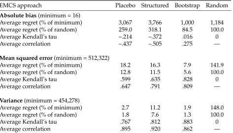
The first result is that performance of both EMCS procedures in terms of bias is very poor. The average regret in terms of absolute bias, as a percentage of the absolute bias

for the best estimator, is 3,067% (3,766%) for placebo (structured), i.e. an order of

mag-nitude larger than the minimum value. It is worse than choosing completely randomly, which would be 1,184% worse than the best estimator, and worse than the bootstrap, 1,000%. Looking at the ranking across estimators, the average Kendall’s tau is –.21 (–.37)

for placebo (structured). So the rankings produced by EMCS are, on average,negatively

correlated with the ranking in the original samples. This is worse than random, which

11_{Precisely, we sample with replacement, and draw replication samples of the same size as the original}

(23)

[image:23.612.75.548.96.367.2]

Table 1: EMCS-validity using different performance metrics

EMCS approach Placebo Structured Bootstrap Random

Absolute bias(minimum = 16)

Average regret (% of minimum) 3,067 3,766 1,000 1,184

Average regret (% of random) 259.0 318.1 84.5 100.0

Average Kendall’s tau –.214 –.372 .016 0

Average correlation –.437 –.505 .275 —

Mean squared error(minimum = 512,322)

Average regret (% of minimum) 18.2 16.3 7.9 141.9

Average Kendall’s tau .599 .635 .828 0

Average correlation .647 .791 .809 —

Variance(minimum = 454,278)

Notes: ‘EMCS approach’ denotes the way in which the empirical Monte Carlo samples were generated.

‘Placebo’ and ‘Structured’ generate samples using the placebo and structured approaches described in Sec-tion 2. ‘Bootstrap’ generates nonparametric bootstrap samples by sampling with replacement the same num-ber of observations as the original data. ‘Random’ does not generate samples but instead randomly assigns

rankingsto the estimators (hence statistics are only available for the performance metrics based on rankings). The absolute bias, mean squared error, and variance are features of estimators. The ‘minimum’ value for each feature is its lowest value among our estimators in the original data generating process (i.e.we have one value of each feature for each estimator in the ‘original samples’ and we report the lowest of these values). See Appendix F in Advaniet al.(2019) for more details. Four performance measures are used for each of these statistics. ‘Average regret’ measures the average increase in the statistic from choosing the estimator actually selected by the EMCS approach rather than the estimator with the minimum value of this statistic, as a percentage of(i)that minimum value or(ii)the average regret for random selection of estimators. ‘Average Kendall’s tau’ measures the average correlation in the ranking of estimators provided by the EMCS approach relative to the ranking in the original samples. ‘Average correlation’ measures the average correlation in the actual values of the statistic (rather than the ranking) provided by the EMCS approach relative to the values in the original samples. All averages are taken with respect to 1,000 original samples; for each sample, a sep-arate simulation study was conducted. The results for random selection of estimators are analytical; instead of actually generating random rankings, we report the known values of expected Kendall’s tau (zero) and expected regret with random rankings. The latter value is equal to the average regret across estimators, with an equal probability of each estimator to be selected as ‘best’.

gives .00, and bootstrap, .02. The same pattern is seen in the average correlation coeffi-cients for absolute bias, which are –.44 (–.51).

(24)

Similarly, average Kendall’s tau is now .60 and .64 for placebo and structured, respec-tively, much better than .00 for random. The lowest panel of Table 1 shows that this is driven by the much better performance in replicating the variances. Since the rankings here are mostly determined by the variance, being able to reproduce variances substan-tially improves the measures of performance relative to the metrics based on absolute bias.

However, looking at our other benchmark case – the bootstrap – we see that it out-performs both EMCS methods in terms of MSE. Average regret is lower at 7.9%, and the average Kendall’s tau is much higher at .83. Given that MSE performance for EMCS is driven by the variance components, this does not seem surprising. The bootstrap is a simpler procedure than the two EMCS methods, and its ability to help us understand the variability of estimators is well known. It therefore seems like a potentially valuable path which has fewer design choices than EMCS.

5.2 Removing Sampling Error from the ‘True Effect’

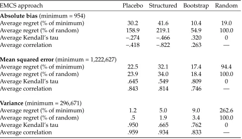
The previous subsection calculated the MSE for each estimator by comparing the value of the estimate in each sample to a ‘true effect’ measured using the experiment. One concern might be that the estimate from the experiment is subject to sampling error, and this might somehow negatively affect our performance measures for EMCS. To test this, we now use as our ‘treated’ observations the ‘early random assignment’ NSW control sample from Smith and Todd (2005). Since these individuals were selected for the programme in the same way as those actually treated, but were then randomised out, the actual treatment effect for them is precisely zero. We therefore repeat the exercise on these data, again implementing the two EMCS procedures 1,000 times on each of the 1,000 original samples.

Table 2 documents the results. Appendix F in Advaniet al.(2019) provides further details.

(25)

boot-Table 2: EMCS-validity ensuring no sampling error in the treatment effect

Average Kendall’s tau –.274 –.466 .320 0

Average correlation –.418 –.822 .263 —

Mean squared error(minimum = 1,222,627)

Average regret (% of random) .5 1.9 3.4 100.0

Notes:See Table 1.

strap (10%). As before, the average Kendall’s tau is negative for placebo (structured) at –.27 (–.47), which is worse than random (.00) and bootstrap (.32) as well. On MSE perfor-mance is better, with average regret of 23% (32%) and average Kendall’s tau of .65 (.55). These are much better than random (94% and .00), but worse than bootstrap (17% and .81).

5.3 Ensuring Unconfoundedness Holds

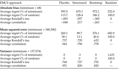
Another potential concern is whether the conditional independence assumption holds. Here we take the approach described in Subsection 4.2 to generate 1,000 samples in which conditional independence holds by construction. Then, we implement the two EMCS procedures 500 times on each of these samples. Table 3 displays the results. Appendix F

in Advaniet al.(2019) provides further details.

[image:25.612.70.551.96.372.2]

(26)

[image:26.612.74.547.96.372.2]

Table 3:EMCS-validity ensuring unconfoundedness holds

Average Kendall’s tau –.003 .057 –.300 0

Average correlation –.048 .217 –.263 —

Mean squared error(minimum = 340,300)

Average regret (% of minimum) 0 .3 0 1,631

Average regret (% of random) 0 0 0 100.0

Notes:See Table 1.

Kendall’s tau is a little higher, so it is also not obvious that contexts where conditional independence holds should necessarily see better performance of EMCS procedures.

6 Discussion

Advances in econometrics have left the empirical researcher blessed with a wealth of pos-sible treatment effect estimators from which to choose. They have not yet provided clear guidance on which of these estimators should be preferred in which context. In this paper we studied two proposals which suggest an approach to choosing an appropriate estima-tor for a given context. The first approach (placebo) suggests a way to introduce placebo treatments to some control observations in a dataset, and studies how well estimators can pick up the true zero effect. The second approach (structured) creates data from a known DGP whose parameters are estimated from features of the original data, and studies how well estimators can pick up the implied true effect in the DGP.

(27)

where one or other of these might fail, and gave an example of the consequences based on simulations from an artificial DGP. To provide a real-world example, we also imple-mented the EMCS procedures in the NSW–CPS data, where we know the ‘true effect’ of the programme. This allowed us to compute actual performance of the estimators in sam-ples from the original data, and compare this to what EMCS would suggest if applied to these samples. We showed that in this example EMCS performs badly on ordering esti-mators in terms of absolute bias, and the estimator it suggests is often many times worse than the best (or even than selecting randomly). In this example both EMCS procedures perform much better in terms of MSE because reproducing the variance term turns out to drive the MSE in these data. But, this leads the methods to be no better (and sometimes substantially worse) than a simple bootstrap procedure.

These results are unfortunate, but nevertheless important. There remains no silver bullet that can assist empirical researchers with the ‘right’ or ‘best’ estimator for a partic-ular context. In the absence of a clear choice driven by research design, the best advice at this stage is likely to be implementing a number of estimators, and then considering the

range of estimates provided, as Bussoet al.(2014) also suggest.

One possible future alternative, recently proposed, is synth-validation (Schuler et al.,

(28)

References

ABADIE, A. AND M. D. CATTANEO(2018): “Econometric Methods for Program

Evalua-tion,”Annual Review of Economics, 10, 465–503.

ABADIE, A., D. DRUKKER, J. L. HERR,ANDG. W. IMBENS(2004): “Implementing

Match-ing Estimators for Average Treatment Effects in Stata,”Stata Journal, 4, 290–311.

ABADIE, A.ANDG. W. IMBENS(2006): “Large Sample Properties of Matching Estimators

for Average Treatment Effects,”Econometrica, 74, 235–267.

——— (2011): “Bias-Corrected Matching Estimators for Average Treatment Effects,”

Jour-nal of Business & Economic Statistics, 29, 1–11.

——— (2016): “Matching on the Estimated Propensity Score,”Econometrica, 84, 781–807.

ADVANI, A., T. KITAGAWA, AND T. SŁOCZYNSKI´ (2019): “Supplementary Appendix for ‘Mostly Harmless Simulations? Using Monte Carlo Studies for Estimator Selection’,” unpublished manuscript.

AUSTIN, P. C. (2010): “The Performance of Different Propensity-Score Methods for

Es-timating Differences in Proportions (Risk Differences or Absolute Risk Reductions) in

Observational Studies,”Statistics in Medicine, 29, 2137–2148.

BERTRAND, M., E. DUFLO, AND S. MULLAINATHAN (2004): “How Much Should We

Trust Differences-in-Differences Estimates?” Quarterly Journal of Economics, 119, 249–

275.

BLUNDELL, R. AND M. COSTA DIAS (2009): “Alternative Approaches to Evaluation in

Empirical Microeconomics,”Journal of Human Resources, 44, 565–640.

BODORY, H., L. CAMPONOVO, M. HUBER, AND M. LECHNER (2018): “The Finite

Sam-ple Performance of Inference Methods for Propensity Score Matching and Weighting

Estimators,”Journal of Business & Economic Statistics, forthcoming.

BREWER, M., T. F. CROSSLEY, AND R. JOYCE (2018): “Inference with

Difference-in-Differences Revisited,”Journal of Econometric Methods, 7.

BUSSO, M., J. DINARDO, AND J. MCCRARY (2009): “Finite Sample Properties of

(29)

——— (2014): “New Evidence on the Finite Sample Properties of Propensity Score

Reweighting and Matching Estimators,”Review of Economics and Statistics, 96, 885–897.

CALONICO´ , S. AND J. SMITH (2017): “The Women of the National Supported Work

Demonstration,”Journal of Labor Economics, 35, S65–S97.

CAMERON, A. C., J. B. GELBACH, ANDD. L. MILLER(2008): “Bootstrap-Based

Improve-ments for Inference with Clustered Errors,”Review of Economics and Statistics, 90, 414–

427.

CHEN, X., H. HONG,ANDA. TAROZZI(2008): “Semiparametric Efficiency in GMM

Mod-els with Auxiliary Data,”Annals of Statistics, 36, 808–843.

DEHEJIA, R. H. AND S. WAHBA (1999): “Causal Effects in Nonexperimental Studies:

Reevaluating the Evaluation of Training Programs,” Journal of the American Statistical

Association, 94, 1053–1062.

——— (2002): “Propensity Score-Matching Methods for Nonexperimental Causal

Stud-ies,”Review of Economics and Statistics, 84, 151–161.

DIAMOND, A. AND J. S. SEKHON (2013): “Genetic Matching for Estimating Causal

Ef-fects: A General Multivariate Matching Method for Achieving Balance in Observational

Studies,”Review of Economics and Statistics, 95, 932–945.

D´IAZ, J., T. RAU, ANDJ. RIVERA(2015): “A Matching Estimator Based on a Bilevel

Opti-mization Problem,”Review of Economics and Statistics, 97, 803–812.

FROLICH¨ , M. (2004): “Finite-Sample Properties of Propensity-Score Matching and

Weighting Estimators,”Review of Economics and Statistics, 86, 77–90.

FROLICH¨ , M., M. HUBER, AND M. WIESENFARTH (2017): “The Finite Sample

Perfor-mance of Semi- and Nonparametric Estimators for Treatment Effects and Policy

Evalu-ation,”Computational Statistics & Data Analysis, 115, 91–102.

GRAHAM, B. S., C. CAMPOS DE XAVIER PINTO, AND D. EGEL (2012): “Inverse

Prob-ability Tilting for Moment Condition Models with Missing Data,” Review of Economic

Studies, 79, 1053–1079.

——— (2016): “Efficient Estimation of Data Combination Models by the Method of

(30)

HAHN, J. (1998): “On the Role of the Propensity Score in Efficient Semiparametric

Esti-mation of Average Treatment Effects,”Econometrica, 66, 315–331.

HANSEN, C. B. (2007): “Generalized Least Squares Inference in Panel and Multilevel

Models with Serial Correlation and Fixed Effects,”Journal of Econometrics, 140, 670–694.

HECKMAN, J. J.ANDV. J. HOTZ(1989): “Choosing Among Alternative Nonexperimental Methods for Estimating the Impact of Social Programs: The Case of Manpower

Train-ing,”Journal of the American Statistical Association, 84, 862–874.

HIRANO, K., G. W. IMBENS, AND G. RIDDER (2003): “Efficient Estimation of Average

Treatment Effects Using the Estimated Propensity Score,”Econometrica, 71, 1161–1189.

HUBER, M., M. LECHNER, AND G. MELLACE (2016): “The Finite Sample Performance

of Estimators for Mediation Analysis Under Sequential Conditional Independence,” Journal of Business & Economic Statistics, 34, 139–160.

HUBER, M., M. LECHNER, AND C. WUNSCH (2013): “The Performance of Estimators

Based on the Propensity Score,”Journal of Econometrics, 175, 1–21.

IMBENS, G. W.ANDJ. M. WOOLDRIDGE(2009): “Recent Developments in the

Economet-rics of Program Evaluation,”Journal of Economic Literature, 47, 5–86.

JANN, B. (2008): “The Blinder–Oaxaca Decomposition for Linear Regression Models,”

Stata Journal, 8, 453–479.

KHWAJA, A., G. PICONE, M. SALM, AND J. G. TROGDON (2011): “A Comparison of

Treatment Effects Estimators Using a Structural Model of AMI Treatment Choices and

Severity of Illness Information from Hospital Charts,” Journal of Applied Econometrics,

26, 825–853.

KLINE, P. (2011): “Oaxaca-Blinder as a Reweighting Estimator,” American Economic

Re-view: Papers & Proceedings, 101, 532–537.

LALONDE, R. J. (1986): “Evaluating the Econometric Evaluations of Training Programs

with Experimental Data,”American Economic Review, 76, 604–620.

LECHNER, M. AND A. STRITTMATTER (2017): “Practical Procedures to Deal with

Com-mon Support Problems in Matching Estimation,”Econometric Reviews, forthcoming.

LECHNER, M.ANDC. WUNSCH(2013): “Sensitivity of Matching-Based Program