DOI:0000
Efficient model comparison techniques
for models requiring large scale data
augmentation
Panayiota Touloupou1, Naif Alzahrani2, Peter Neal2, Simon E.F. Spencer1 and Trevelyan J. McKinley3
1Department of Statistics, University of Warwick, Coventry, CV4 7AL, UK
2Department of Mathematics and Statistics, Lancaster University, Lancaster, LA1 4YF, UK
3College of Engineering, Mathematics and Physical Sciences, University of Exeter, Penryn Campus, Penryn, Cornwall, TR10 9EZ, UK
Abstract: Selecting between competing statistical models is a challeng-ing problem especially when the competchalleng-ing models are non-nested. In this paper we offer a simple solution by devising an algorithm which combines MCMC and importance sampling to obtain computationally efficient esti-mates of the marginal likelihood which can then be used to compare the models. The algorithm is successfully applied to a longitudinal epidemic data set, where calculating the marginal likelihood is made more challeng-ing by the presence of large amounts of misschalleng-ing data. In this context, our importance sampling approach is shown to outperform existing methods for computing the marginal likelihood.
Keywords and phrases:Epidemics, marginal likelihood, model evidence, model selection, time series.
1. Introduction
The central pillar of Bayesian statistics is Bayes’ Theorem. That is, given a pa-rameteric modelMwith parametersθ= (θ1, . . . , θd) and datax= (x1, x2, . . . , xn),
the joint distribution of (θ,x) satisfies
π(θ|x)π(x) =π(x|θ)π(θ). (1)
The four terms in (1) are the posterior distributionπ(θ|x), the marginal like-lihood or evidenceπ(x), the likelihoodπ(x|θ) and the prior distribution π(θ). The terms on the right hand side of (1) are usually easier to derive than those on the left hand side. The statistician has considerable control over the prior distribution and this can be chosen pragmatically to reflect prior beliefs and to be mathematically tractable. For many statistical problems the likelihood can easily be derived. However, the quantity of primary interest is usually the pos-terior distribution. Rearranging (1) it is straightforward to obtain an expression for π(θ|x) so long as the marginal likelihood can be computed. This involves computing
π(x) =
Z
π(x|θ)π(θ)dθ, (2)
which is only possible analytically for a relatively small set of simple models. A key solution to being unable to obtain an analytical expression for the posterior distribution is to obtain samples from the posterior distribution using Markov chain Monte Carlo (MCMC;Metropoliset al.,1953;Hastings,1970). A major strength of MCMC is that it circumvents the need to computeπ(x) and this has led to its widespread use in Bayesian statistics over the last 25 years or so. However, Bayesian model choice typically requires the computation of Bayes Factors (Kass and Raftery, 1995) or posterior model probabilities, which are both functions of the marginal likelihoods for the competing models. In Chib (1995) a simple rewriting of (1) was exploited to obtain estimates of the marginal likelihood using output from a Gibbs sampler. This has been extended inChib and Jeliazkov(2001) andChen(2005) to be used with the general Metropolis-Hastings algorithm. Importance sampling approaches to estimating the marginal likelihood have also been suggested (Gelfand and Dey, 1994), along with gen-eralisations such as bridge sampling (Meng and Wong, 1996), which ‘bridges’ information from posterior and importance samples. More recently approaches have exploited the ‘thermodynamic integral’ such as power posterior methods Friel and Pettitt(2008). Alternative methods such as Sequential Monte Carlo (e.g.Zhouet al.,2015) and nested sampling (Skilling,2004) do not require any MCMC: computation of the marginal likelihood and samples from the poste-rior distribution are produced simultaneously. A potential drawback for many of the above approaches to marginal likelihood estimation is that it may not be obvious how to apply them efficiently to models incorporating large amounts of missing data.
It should be noted that there are model comparison techniques such as re-versible jump (RJ)MCMC (Green, 1995) which can used to compare models without the need to compute the marginal likelihood. RJMCMC works well for nested models where it is straightforward to define a good transition rule for models with different parameters. However, in the case where we have large amounts of missing data it is often necessary to use some form of data augmen-tation technique, where the missing information is inferred alongside the other parameters of the model. Using RJMCMC becomes much harder in these cases since the dimension of the parameter space (including the augmented data) be-comes large. This is exacerbated further when the missing information between the competing models has a different structure. In this latter case the use of in-termediary (bridging) models (Karagiannis and Andrieu,2013) to move between the models of interest is a possibility.
parameters and augmented data (random effects terms) assists tremendously in devising an efficient estimator of the marginal likelihood. In Section 4 we consider final outcome household epidemic data where in the special case of the Reed-Frost model exact, but expensive, computation of the marginal likelihood is possible for comparison purposes. In Section5we apply the methodology to an epidemic example, for the transmission ofStreptococcus pneumoniae(Melegaro
et al., 2004) comparing our algorithm to existing methods for computing the marginal likelihood demonstrating its simplicity and effectiveness in the presence of missing data. Finally in Section6we briefly discuss extensions and limitations of the algorithm.
2. Algorithm
Our starting point in the estimation ofπ(x) is to note that we can rewrite (2) as
π(x) =
Z
θ
π(x|θ)π(θ)
q(θ)q(θ)dθ, (3)
where q(θ) denotes a d-dimensional probability density function. We assume that if π(θ) > 0 then q(θ) > 0. Then an unbiased estimator, Pbq of π(x) is
obtained by samplingθ1,θ2, . . . ,θN from q(θ) and setting
b
Pq =
1 N
N
X
i=1
π(x|θi)
π(θi)
q(θi)
. (4)
Thus Pbq is an importance sampled (see, for example, Ripley, 1987) estimate
of π(x), and the effectiveness of the estimator given by (4) depends upon the variability ofπ(x|θ)π(θ)/q(θ).
The remainder of the paper and this Section, in particular, is focussed on how we can effectively exploit (4) in the estimation of π(x). The first observation is that the optimal choice of q(θ) is π(θ|x), the posterior density but if we knew this, thenπ(x) would also be known. A simple solution is to use output from an MCMC algorithm to inform the proposal distribution (Clyde et al., 2007). For most statistical models the likelihood times the prior is unimodal for sufficiently largen. In these circumstances, the posterior distribution ofθis almost always approximately Gaussian with meanbθ, the posterior mode, and
covariance matrix Σ = −I(θ)b −1, where I(θ) denotes the Fisher information
a “defense mixture” (Hesterberg,1995),
qD(θ) =pφ(θ;µ,Σ) + (1−p)π(θ). (5)
where φ(·;µ,Σ) is the probability density function of a multivariate Gaussian distribution with meanµand covariance matrix Σ, estimated from the MCMC output, and p is a mixing proportion. This proposal ensures that the ratio of the prior density to the proposal density is bounded above by 1/(1−p) withptypically chosen to be 0.95. We found that at-distribution proposal was preferable in Sections 3 and 4, whereas the defense mixture proposal was the preferred choice in Section5.
We are now in position to outline the three step algorithmic procedure, which is implemented in the paper followed by highlighting the scope and limitation of the approach. The steps are as follows:
1. Obtain a sample θ1,θ2, . . . ,θK from the (approximate) posterior
distri-bution,π(θ|x). Throughout this paper, and in practice, this will generally be achieved using MCMC withK chosen such that the sample is repre-sentative of the posterior distribution. However, any alternative method for obtaining an approximate sample from the posterior distribution could be used.
2. Use the sampleθ1,θ2, . . . ,θK to derive a parametric approximation of the
posterior distribution and let q(·) denote the corresponding probability density function. For example, choosing q(·) either to be a multivariate t-distribution or a “defense mixture” will usually work well.
3. Sample ˜θ1,θ˜2, . . . ,˜θN fromq(·). (The tilde notation is used to distinguish
the sample obtained fromq(·) from the sample used to estimateq(·).) For eachi= 1,2, . . . , N, computeπ(x|θ˜i) and estimateπ(x) using (4).
In situations whereπ(x|θ) is analytically available, the construction of an MCMC algorithm to sample fromπ(θ|x) will be straightforward and implementation of the algorithm will be trivial. Then the procedure becomes a simple and fast ap-pendage to a standard MCMC algorithm. However, assuming an independent and identically distributed sample from q(·), the variance of the importance sampling estimator given in (4) is given by
Var(Pbq) =N−1
Z
π(x|θ)π(θ) q(θ) −π(x)
2
q(θ)dθ
=N−1π(x)2
Z π(θ|x)
q(θ) −1
2
q(θ)dθ,
that a dependent sample fromq(·) in Step 3 of the algorithm can be exploited to reduce the variance of the estimator. A prime example is the defense mix-ture proposal wherepN and (1−p)N samples are drawn from the multivariate Gaussian distribution and the prior, respectively.
The motivation for the work are in circumstances whereπ(x|θi) is not readily
available, see Sections3 and 5, and further work is required to implement the algorithm. Whenπ(x|θ) is not available, it is often possible, with the addition of augmented data y, to obtain an analytical expression for π(x,y|θ). This can then be utilised within an MCMC algorithm to obtain samples from the joint posteriorπ(θ,y|x). Devising an importance sampling proposal distribution q(θ,y) approximating π(θ,y|x) will not be practical ify is high-dimensional, for example, the dimension ofyis equal to or greater ton, the dimension ofx. See, for example, Section3for limitations of this approach. The solution that we propose is to use the marginal MCMC output fromπ(θ|x) to inform the proposal distribution q(θ) in the importance sampling above, and then to separately consider the computation of π(x|θ), which will be largely problem specific. In the linear mixed model example in Section 3, the distribution of yi (random
effect term) is readily available givenθ and xi, and hence we can sample the
random effectsyfrom their full conditional distributions. This approach extends to the epidemic model in Section5, whereyrepresents the unobserved infectious status of individuals with respect toStreptococcus pneumoniae carriage and the Forward Filtering Backwards Sampling (FFBS) algorithm (Carter and Kohn, 1994) can be used to calculateπ(y|x,θ), and hence π(x|θ). In future work we will show how particle filtering, (Gordonet al.,1993), can be applied to estimate π(x|θ) extending the scope of the algorithm with particular reference to Poisson regression models (Zeger, 1988). The estimation of π(x|θ) can be potentially computationally costly and thus the overall cost of the algorithm needs to be considered. However, the computation of the {π(x|θ˜i)}’s can, in contrast to
the MCMC runs, be undertaken in parallel, which can ease the computational burden.
Our approach can be used to estimate Bayes’ Factors in objective model selec-tion where for two competing models, common model parameters are assigned improper, non-informative priors. Consider two competing modelsM1andM2
with parametersθ1= (φ,ω1) and θ2 = (φ,ω2), respectively, and letφdenote
parameters common to both models. Let Φ⊆Rd denote the sample space for
φ. Suppose that a common priorπ0(φ) is chosen forφin both models and that
the prior forMk (k= 1,2) factorises as πk(θk) =π0(φ)πk1(ωk), whereπk1(·)
is assumed to be a proper probability density. We can then chooseφ0∈Φ as a reference point and set ˜π0(φ0) = 1 and for allφ∈Φ, set ˜π0(φ) =π0(φ)/π0(φ0).
Let
πk(x) =
Z Z
πk(x|φ,ωk)π0(φ)πk1(ωk)dφdωk, (6)
and
˜ πk(x) =
Z Z
Then letting B12 = π1(x)/π2(x) denote the Bayes’ Factor between models 1
and 2, it follows from (6) and (7) that
B12=
π1(x)
π2(x)
=π˜1(x) ˜ π2(x)
. (8)
Therefore it suffices to estimate ˜πk(x) (k= 1,2) in order to estimateB12. The
estimation of ˜πk(x) can proceed along the same lines asπk(x) in (4) by selecting
a proper proposal densityqk(·) and using samples (φk1,ωk1), . . . ,(φ k
N,ωkN) from
qk(·) to estimate ˜πk(x) by
e
Pqk = 1 N
N
X
i=1
πk(x|φki,ω k i)
˜
π0(φki)πk1(ωki)
qk(φki,ωki)
. (9)
In this case the “defense mixture” proposal is inappropriate but a multivariate t-distribution can be used as an effective proposal distribution.
In our approach each model is required to be analysed separately and the computational cost increases approximately linearly in the number of models to be compared. Therefore this approach is not competitive for comparing large numbers of nested models, for example, the inclusion or exclusion ofpcovariates in a generalised linear model, a situation where reversible jump MCMC (Green, 1995) can be effectively applied. Our approach is more suited to comparing a small number of competing models which potentially have rather different dy-namics such as integer valued autoregressive (Neal and Subba Rao, 2007) and Poisson regression (Zeger,1988) models for integer valued time series, an exam-ple which we will present in future work. The approach is particularly suited to situations which allow the posterior distribution of the parameters to be approx-imately Gaussian, assisting in the constructionq(·), but this assumption can be relaxed. Furthermore, the appropriateness of a Gaussian, or t-distribution ap-proximation of the posterior can easily be assessed from the MCMC output.
3. Linear mixed model
We illustrate our methodology on the linear mixed model. In particular we may wish to ask the model choice question of whether it is necessary to include a random effect in the model or not. This question would be extremely challenging to address using reversible jump MCMC because it would require an efficient proposal distribution for the complete set of random effects when jumping be-tween models. However it is straightforward to fit both models using MCMC due to the availability of a Gibbs sampler. The full conditional distribution of the random effects then unlocks an efficient importance sampling algorithm for the calculation of the marginal likelihood.
The simplest linear mixed model takes the following form. Let the data be divided intomunits or clusters, and assume that
fori = 1, . . . , m and j = 1, . . . , ni, where ij ∼N(0, σ2) are independent and
identically distributed errors. We assume that the random effects satisfyδi|φ∼
N(0, φ2) and are independent conditional on the standard deviation parameter
φ. The vector of unknown parameters for the model is given byθ= (β, σ,δ, φ). LetZdenote the design matrix of the fixed effects, with rowszT
ij and letWbe
the design matrix for the random effects, so thatx=Zβ+Wδ+. For a review of Bayesian approaches to generalized linear mixed models, see for exampleFong
et al.(2010).
3.1. Simulation study
To illustrate the application of our importance sampling technique we performed a simulation study where the true model is known. We simulated data form= 50 clusters, each containingni= 3 observations, givingn= 150 in total. We
gener-ated 3 predictor variables for each cluster by drawingmvalues from a standard normal distribution. We fixed our true parameters to be βT = (10,−20,30), σ= 1 andφ= 2. For every cluster we assumed the same predictors and drew a random effectδifromδi|φ∼N(0, φ2). Finally, the observed datax= [xij] were
drawn from equation (10).
3.2. Model 1 – with random effects
For the fixed effects we chose Zellner’sg-prior (Smith and Kohn,1996), namely β|σ ∼ N(0, gσ2(ZTZ)−1). In our application we chose g = n, known as the
unit information prior (Kohnet al.,2001). For the variance parameters we used inverse gamma priors:σ2 ∼IG(a
σ, bσ) and φ2 ∼IG(aφ, bφ), setting these
pa-rameters equal to 1 in our implementation. These conjugate priors allow a Gibbs sampling algorithm to sample from the posterior distribution. The full condi-tional distributions are given by,
β, σ2|x,δ∼N IG(m∗,V∗, a∗, b∗) (11)
m∗= g 1 +g(Z
TZ)−1ZT(x−Wδ)
V∗= g 1 +g(Z
TZ)−1
a∗=aσ+
n
2 (12)
b∗=bσ+
1
2(x−Wδ)
T
In−
g 1 +gZ(Z
TZ)−1ZT
(x−Wδ) (13)
φ|δ∼IG(aφ+m2, bφ+12δTδ) (14)
δi|x,β, σ, φ∼N
1 κi
ni
X
j=1
xij−zTijβ, κ −1 i
(15)
κi=φ12 +
ni
After a burn-in of 1000 iterations, we drew 10000 samples from the MCMC. To demonstrate the increased efficiency provided by making use of the approach to handle missing data described in Section 2, we considered two importance sampling estimators.
3.2.1. Full posterior importance sampling
In the full posterior importance sampler, we estimate the mean and covariance matrix for the full parameter vectorθincluding the random effects, givingm+5 parameters in total. We then used these as the centre and scale matrix for multivariate t-distributed proposal distribution with 5 degrees of freedom, with densityq1(θ). We drew N = 1000 samples from this proposal, denoting them
by{θi}Ni=1. The importance sampling estimator is thenPbq1 given in (4).
3.2.2. Marginal posterior importance sampling
In the second importance sampling approach we make use of missing data tech-nique described in Section 2. We calculate the marginal mean and covariance matrix for the (restricted) parameter vectorψ = (β, σ, φ). Again we use these as the centre and scale matrix for a multivariate t-distributed proposal with 5 degrees of freedom, but this time it has just 5 dimensions. For eachψi that is drawn from the proposalq2(ψ), we sample the random effectsδi from their full
conditional distribution in Equation (15). The importance proposal is therefore given byq2(ψ)π(δ|x,ψ).
Note that in both of these estimators we have chosen to parameterise our proposal distribution in terms of the standard deviations (σandφ) rather than the variances in order to lighten the tails. However since the priors are written in terms of the variance parameters we must multiply the proposal densities q1(θ) andq2(ψ) by the Jacobianσφ/4 to obtain the correct marginal likelihood
estimator.
3.3. Model 0 – without random effects
The model with no random effects is just a linear model, given byxij=zTijβ+ij.
We assume the same conjugate priors forβandσ2described in Section3.2and
in this case the marginal likelihood may be calculated analytically, namely,
π(x) = b
aσ
σ Γ(a∗)
(2π)n/2Γ(a σ)
(b∗)−a∗,
3.4. Results
-425.5 -425.4 -425.3 -425.2 -425.1 -425.0 Log marginal likelihood
Full posterior IS for lmm Marginal posterior IS for lmm Linear model IS
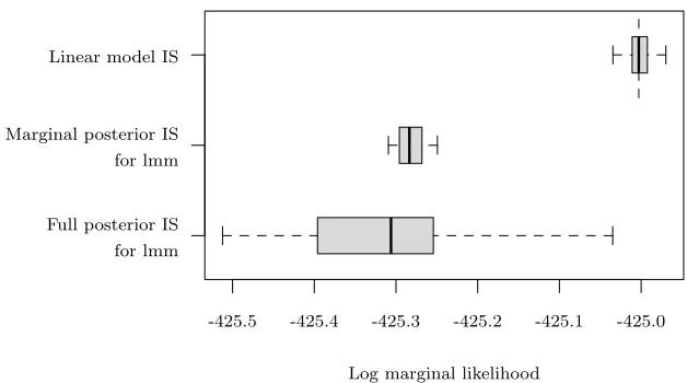
Fig 1. Variation of the log marginal likelihood estimates for the linear model and linear mixed model (lmm) over 50 replicates. For the lmm, in the full posterior approach the whole parameter vector (including random effects) was approximated in the importance proposal; in the marginal posterior approach the random effects were left out, and drawn from their full conditional distribution. A dashed vertical line indicates the true log marginal likelihood for the linear model.
Figure1shows the variation in 50 Monte Carlo replicates of each importance sampling estimator, based on 1000 samples. The importance sampling estimates for the linear model fall close to the true log marginal likelihood value, indicated by a dashed vertical line. For the linear mixed model treating the random effects as missing data and drawing them from their full conditional distribution greatly reduces the variance of the importance sampling estimator. The Monte Carlo standard errors for the linear model and linear mixed model with missing data were 0.0123 and 0.0171, compared with 0.106 for the linear mixed model with an importance proposal for the full parameter vector.
When we increase the number of clusters m from 50 to 500 (Figure 2 of the supplementary material) the Monte Carlo standard error for the marginal posterior approach was 0.015, showing no increase due to the increase in missing data. For comparison, the Monte Carlo standard error for the full parameter importance sampling approach increased to 0.825 form= 500.
[image:9.612.149.463.167.342.2]envisage situations in which this loss of precision could lead to an incorrect conclusion.
4. Final outcome epidemic data
In this Section, we look at applying the methodology developed in Section2to final outcome household epidemic data. Specifically, we assume that the data consist of the number of individuals infected during the course of an epidemic in a number of households of various sizes. We follow Addy et al. (1991) and Neal and Kypraios(2015) in assuming that the epidemics in each of the house-holds are independent with each member of a household having probabilitypG
of being infected globally from the community at large and the within household epidemic spread emanating from the individuals infected globally. Within each household the disease dynamics are assumed to follow a homogeneously mix-ing, generalised stochastic epidemic model, where infectious individuals have independent and identically distributed infectious periods according to an arbi-trary, but specified, non-negative probability distributionQwithE[Q] = 1 and during their infectious period make contact with a given susceptible in their household at the points of a homogeneous Poisson point process with rateλL.
The special case whereQ ≡ 1 has the same final outcomes in terms of those infected as a household Reed-Frost model within household infection probabil-ity pL = 1−exp(−λL). Throughout we assign an Exp(1) prior to λL which
corresponds to aU(0,1) prior onpL and also aU(0,1) prior onpG.
For the household Reed-Frost epidemic it is trivial to adapt the approach of Neal and Kypraios (2015), Section 3.3 to compute the marginal likelihood exactly. Details of how this can be done are given in the supplementary mate-rial. Therefore we are able to compare our estimation of the marginal likelihood with the exact marginal likelihood. The exact computation of the marginal like-lihood grows exponentially in the total number of households whilst the MCMC algorithm for estimating the parameters and the algorithm for estimating the marginal likelihood have essentially constant computational cost for a given maximum household size. Therefore the exact computation of the marginal like-lihood is only practical for data containing a small number of households and we apply it to the influenza data sets from Seattle, reported in Fox and Hall (1980), which contain approximately 90 households each.
Exact computation of the marginal likelihood is not possible for generalQ. Therefore we use our approach to compare three different choices of infectious period Q ≡ 1, Q ∼ Gamma(2,2) and Q ∼ Exp(1) to study which infectious period distribution is most applicable for a given epidemic data set. This mimics analysis carried out inAddyet al.(1991) in a maximum likelihood framework where two infectious periods, a constant and a gamma with shape parameter 2, were compared for a combined data set of two influenza outbreaks in Tecumseh, Michigan, seeMontoet al.(1985).
Let x denote the observed epidemic data. The recursive equations given in Ball et al. (1997), (3.12), can be used to compute Ph
0,1, . . . , h), the probability of observingkindividuals out ofhbeing infected in a household of sizeh. Therefore it is straightforward to computeπ(x|λL, pG) or
π(x|pL, pG) for the Reed-Frost model. Consequently, it is trivial to construct a
random walk Metropolis algorithm to sample fromπ(λL, pG|x) (orπ(pL, pG|x)
for the Reed-Frost model) and to estimate the marginal likelihood using samples from a proposal densityq(λL, pG), which is a multivariatetdistribution with 10
degrees of freedom and mean and covariance matrix obtained from the MCMC samples.
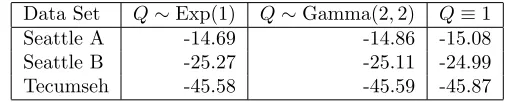
We applied the algorithm for estimating the marginal likelihood to the two Seattle data sets and the Tecumseh data set for each of the three infectious pe-riod distributions. In all cases we ran the MCMC algorithm for 11000 iterations discarding the first 1000 iterations as burn-in and then used 1000 samples to estimate the marginal likelihood. For the Seattle influenza A data set with max-imum household size of 3 it took approximately 2.4 seconds to compute each marginal likelihood in R on a desktop PC with Intel i5 processor. For the Seat-tle influenza B data set and the Tecumseh data set with maximum household size of 5 it took approximately 5 seconds to compute each marginal likelihood. The log marginal likelihoods are given in Table 1, they show that is little in-formation in the data to choose between differentQ, agreeing with findings in Addyet al.(1991) andBall et al.(1997). InterestinglyQ∼Exp(1) is preferred for the Seattle influenza A and Tecumseh data sets, whereasQ≡1 is Seattle influenza B data set. For the two Seattle data sets we also computed the exact log marginal likelihoods, -15.08 and -24.98, for the household Reed-Frost model applied to the Seattle influenza A and influenza B data sets, respectively. For the Seattle data sets we repeated the estimation of the log marginal likelihood 100 times for the Reed-Frost model to obtain Monte Carlo standard errors for the estimated log marginal likelihoods of 0.0062 and 0.0073 for the Seattle in-fluenza A and Seattle inin-fluenza B data sets, respectively, demonstrating good agreement between the estimated and exact log marginal likelihoods. The calcu-lations of the exact marginal likelihood took approximately 0.5 and 14 seconds for the Seattle influenza A and influenza B data sets, respectively. The code for computing the exact marginal likelihood could not be applied to the combined Tecumseh data set, or even the separate Tecumseh data sets (see, for example Clancy and O’Neill,2007) since enumerating over all possible augmented data states exceeded R’s memory allocation. This problem could be circumvented to some extent using sufficient statistics as inNeal and Kypraios (2015) but the current approach offers a simple and fast alternative.
[image:11.612.177.432.562.613.2]Data Set Q∼Exp(1) Q∼Gamma(2,2) Q≡1 Seattle A -14.69 -14.86 -15.08 Seattle B -25.27 -25.11 -24.99 Tecumseh -45.58 -45.59 -45.87
Table 1.Estimated log marginal likelihood for the three influenza data sets using the three choices of infectious period distribution;Q∼Exp(1),
5. Longitudinal epidemic model
5.1. Introduction
In this Section, we explore the application of the methodology developed in Sec-tion2to a scenario whereπ(x|θ) is not readily available, and data augmentation is required both with in the MCMC algorithm and estimation of the marginal likelihood. The example used is based on a longitudinal household study of preschool children under 3 years old and all household members was conducted in the United Kingdom from October 2001 to July 2002 (Hussainet al.,2005). The size of the families varied from 2 to 7, although in most there were 3 or 4 members. All family members were examined forStreptococcus pneumoniae carriage (Pnc) using nasopharyngeal swabs once every 4 weeks over a 10-month period. The carriage status of each individual was recorded at each occasion as 1, if a carrier or 0, if a non-carrier.
FollowingMelegaroet al.(2004), we consider an Susceptible-Infected-Susceptible (SIS) epidemic model for the transmission of Pnc within a household. At any given time, an individual is assumed to be in either the susceptible non-carrier state 0, or the infectious carrier state 1. The population is divided into two age groups, children under 5 years old and everyone else greater than 5 years (whom for brevity we refer to as ‘adults’), denoted by i = 1,2, respectively. LetI1(t) andI2(t) denote the numbers of carrier children and carrier adults in
the household at timet. The transition between state 0 and 1 is referred to as an infection and the reverse transition is referred to as clearance. The transi-tion probabilities between states in a short time intervalδt are defined for an individual in the age groupi:
P(Infection in (t, t+δt]) = 1−exp
−
ki+
β1iI1(t) +β2iI2(t)
(z−1)w
δt
(16)
P(Clearance in (t, t+δt]) = 1−exp(−µi·δt), (17)
whereµi andki are the clearance and the community acquisition rates
respec-tively for age groupiandzis the household size. The rateβijis the transmission
rate from an infected individual in age groupito an uninfected individual in age groupj. The term (z−1)win (16) represents a density correction factor, where
wcorresponds to the level of density dependence and (z−1) is the number of other family members in a household sizez. For example,w= 1 represents fre-quency dependent transmission, where the average number of contacts is equal for each individual in the population. Finally, the probability of infection at the initial swab is assumed to beπi for age groupi. We refer to this model asM1.
approach adopted in this paper to overcome this issue is to use Bayesian data augmentation methods. Model fitting is performed within a Bayesian frame-work using an MCMC algorithm, imputing the unobserved carriage states in each household. LetOj⊆ {1,2, . . . , T}denote the set of prescheduled
observa-tion times of household j = 1,2, . . . , J, and let Uj ={1,2, . . . , T} \Oj denote
the unobserved times. Letxj,t be the binary vector of carriage states for
indi-viduals in household j at observation time t. The observed longitudinal data X = [xj,t]t∈Oj;j=1,...,J consists of the household carriage statuses xj,t at the
observation times. Similarly letyj,tbe the corresponding latent carriage status
of householdj at timet∈Uj, and form the corresponding missing data matrix
Y= [yj,t]t∈Uj;j=1,...,J. Let θ denote the vector of model parameters, including
the rates of acquiring and clearing carriage, the density correctionw and the initial probabilities of carriage.
The remainder of this Section is structured as follows. In Sections 5.2 and 5.3, we introduce the MCMC algorithm and importance sampling algorithms, respectively, required to implement our approach. In particular, we introduce the Forward Filtering Backward Sampling algorithm (Carter and Kohn, 1994) to assist with dealing with the augmented datay. In Sections5.4and 5.5 sulated data (where the true model is known) are used to illustrate the im-plementation, performance and applicability of the proposed method and its comparative performance against a range of alternatives. We demonstrate that for a fixed computational cost our approach performs at least as well as existing methods, and with the exception of bridge sampling (Meng and Wong,1996), performs considerably better.
5.2. Markov chain Monte Carlo algorithm
In the Bayesian approach, the missing data is represented as a nuisance param-eter and inferred from the observed data like any other paramparam-eter. The joint posterior density of the latent carriage states y, and the model parameters θ can be factorized as:
π(y,θ|x)∝P(y,x|θ)π(θ)
=π(θ)
J
Y
j=1 T
Y
t=1
P(zj,t|zj,t−1,θ),
wherezj,t equals xj,t ift∈Oj; yj,t ift∈Uj and∅ ift = 0. This factorization
is based on the assumption that conditionally on the model parameters, the carriage process is assumed to be independent across households.
zj,t+1,xj,Oj∩{1:t},θ) for eacht∈Uj working forwards in time. The second part
then works backwards through time, simulating yj,t from these conditionals,
starting witht= max(Uj) and ending witht= min(Uj). The model parameters
π1 andπ2 are updated using Gibbs updates and the remaining parameters are
updated jointly using an adaptive Metropolis-Hastings random walk proposal (Roberts and Rosenthal,2009).
5.3. Marginal likelihood estimation via importance sampling
The availability of the full conditional distribution of the missing dataP(y|x,θ) from the FFBS algorithm allows the missing data componenty to be updated using a Gibb’s step in the MCMC algorithm. This full conditional can be ex-ploited further in the estimation of the marginal likelihood. We requireP(x|θ) in order to form the importance sampling estimator in (4). Using Bayes’ Theorem we can rewrite this as
P(x|θ) = P(x|y,θ)P(y|θ) P(y|x,θ) =
P(x,y|θ)
P(y|x,θ), (18)
for anyysuch that P(y|x,θ)>0. Therefore evaluation of P(x|θ) at the point θ can be done by evaluating the right-hand-side of (18) with any suitabley. A suitabley is guaranteed if it is sampled from the full conditional distribution y|(x,θ).
Our approach proceeds as follows. In step 1 we use MCMC to obtain samples from the joint posterior ofθandy. In step 2 we fit a multivariate normal distri-bution to the posterior samples forθonly, and use it to construct a normalised proposal densityq(θ). In step 3, we obtain N samples fromq(θ) and for each sampleθi we obtain a corresponding sample for the missing data yi using the
Forward Filtering Backward Sampling algorithm. We then use these samples to calculate the importance sampling estimator of the marginal likelihood:
b
Pq(x) =
1 N
N
X
i=1
P(x,yi|θi)
P(yi|x,θi)
π(θi)
q(θi)
. (19)
The choice ofq(θ) is important for the accuracy and computational efficiency of the importance sampling approach. As discussed earlier, we wantq(θ) to be a good approximation ofπ(θ|x) but with heavier tails to ensure that the variance ofPbq is small. We therefore investigate a range of proposals distributions based
on a fitted multivariate normal distribution with meanµand covariance matrix Σbased on the MCMC output. These include drawingθfromISNj :N(µ, jΣ)
(j = 1,2,3), a multivariate Normal distribution with different variances;IStd:
td(µ,Σ) (d= 4,6,8), a multivariate Student’st distribution with ddegrees of
freedom, mean µand covariance matrix d−d2Σ (ifd > 2) and ISmix : q(θ) =
5.4. Marginal likelihood estimation
We consider the problem of estimating the marginal likelihood under the model introduced in Section5.1, using the methods described above. These estimators were evaluated on synthetic data analogous to the real data inMelegaro et al.
(2004). More specifically, the parameter values were based on the maximum likelihood estimates from the analysis of Pnc data; parameters were chosen to be k1 = 0.012, k2 = 0.004, β11 = 0.047, β12 = 0.005, β21 = 0.106, β22 =
0.048, µ1 = 0.020, µ2 = 0.053, w = 1.184, π1 = 0.425 and π2 = 0.095. We set
the time-intervalδt= 7. Only complete family transitions, where the infection state of all household members was known on two consecutive observations, were used previously (Melegaro et al., 2004; 51% of the full dataset). Although our approach could easily handle the missing data, for comparability we match the number of complete transitions by family size and number of adults to generate our data set; a total of 66 families comprising 260 individuals including 94 children under 5 years. The simulations were designed so that real and simulated datasets have the same sampling times. The hidden variableyconsists of 1650 yj,t’s, comprising 6500 unobserved binary variables in total.
We compare the proposed importance sampling approach for estimating the marginal likelihood (based on the 7 proposal densities) with bridge sampling (Meng and Wong,1996) (using the importance samples fromISmix), harmonic
mean (Newton and Raftery,1994), Chib’s method (Chib,1995; Chib and Jeli-azkov,2001) and the power posteriors method (Friel and Pettitt,2008). Details of the computation of these estimators are given in the supplementary material. To compare the different methods on a fair basis, we chose to dedicate equivalent amounts of computational effort for estimation of the log marginal likelihood, instead of fixing the total number of samples.
Implementation details are given as follows. The construction of the impor-tance density was based on 25000 MCMC samples after a burn-in of 5000, obtained from the MCMC sampler described in Section 5.2. These posterior samples were used to estimate the reference parametersµ and Σ for a multi-variate Student’stor normal proposal density. The marginal likelihood estimate was then based on 25000 importance sampling draws from the obtained proposal densityq(θ), using the estimator in (19). To produce the bridge sampling esti-mate, the 25000 samples fromISmix were combined with 250 thinned samples
from the MCMC. In order to apply Chib’s methods, the same posterior sam-ples were used for computing the high posterior density point. The log marginal was estimated by generating 22000 draws in each complete and reduced MCMC run, with the first 2000 draws removed as burn-in. Harmonic mean analysis was based on 50000 posterior samples, following a 3000 iteration burn-in. For the power posterior method, it was necessary to specify the temperature scheme and a pilot analysis (not counted in the computation cost) was used to choose 20 partitions on the unit interval. The MCMC sampler was run for 2650 iterations for each temperature in the descending series, omitting the first 650 as burn-in, finishing with 2650 samples att= 0 (the prior).
estimate of the variation in each approach. We also vary the total running time in order to investigate the effect of this on the accuracy of the marginal like-lihood estimates, see Table 1 in the supplementary material. For each analysis method we used the same priors: Gamma(0.01,0.01) for the density factor w; Beta(1,1) for the initial probabilities of infection π1 and π2 and Gamma(1,1)
for the remaining parameters.
HM PP Chib ISmix
-931 -927 -923 -919 -1238 -1235 -1232
Log marginal likelihood
BSmix ISmix ISt8
ISt6
ISt4
ISN3
ISN2
ISN1
-1237.3 -1237.1 Log marginal likelihood
Fig 2. Left: Boxplots of the estimated log marginal likelihood for modelM1 over 50 replicates for our importance sampling approach with the mixture proposal (ISmix), Chib’s method
(Chib), power posteriors method (PP) and harmonic mean (HM) (note the different scales for the top and bottom plots). Right: Zoomed in boxplots of the estimated log marginal likelihood for model M1 over 50 replicates for each of our importance sampling approach (ISN1, ISN2, ISN3, ISt4, ISt6, ISt8, ISmix) and bridge sampling (BSmix).
Figure 2 shows the variability of the eleven marginal likelihood estimators. Except for the harmonic mean, all the methods appear to have produced con-sistent estimates of the marginal likelihood. Chib’s method produced better estimates of the marginal likelihood than the power posterior method, which is more computationally expensive than the other methods and therefore uses a small number of MCMC samples at each temperature, leading to large uncer-tainty. However as seen in Figure 2, the bridge sampling and the importance sampling methods offer significant improvements in precision over the other methods. Moreover, increasing the number of samplesN, led to a decrease in the Monte Carlo standard errors of order O(√N), see Table 1 in the supple-mentary material, indicating that the variances of the corresponding estimators are finite.
[image:16.612.152.458.203.393.2]density. More surprisingly we were unable to use the bridge sampling technique to improve substantially on the standard errors, which dropped from 0.0196 for ISmixto 0.0179 forBSmix. The bridge sampling estimator attempts to combine
information from the MCMC and importance samples, however the optimal estimator is derived assuming that independent samples from the posterior were available, which we approached by applying a thinning of 100 to the samples. With low levels of thinning (results shown in supplementary material Figure 4) we found that bridge sampling actually increased the standard error of the marginal likelihood estimate.
On the basis of this example, the lowest variance importance sampling esti-mator was obtained using the proposal densityISmix – a mixture of the prior
and the normal fitted to the posterior samples. Therefore, in the next section we use this proposal density when estimating the log marginal likelihood via importance sampling.
5.5. Model comparison
In this Section, we apply the marginal likelihood estimation approaches to the problem of Bayesian model choice. We focus on their ability to distinguish be-tween biologically motivated hypotheses concerning the dynamics of Pnc trans-mission. In particular we compare their performance against the established technique of Reversible Jump Markov Chain Monte Carlo (RJMCMC) and then demonstrate that the importance sampling approach can solve problems that are extremely challenging with RJMCMC. We show that using our approach it is possible to answer the epidemiological important question of how household size is related to transmission with extended discussion given in the supplementary material.
Suppose that we wish to evaluate the evidence in favour of the community acquisition rates being equal for adults and children, in the hope of developing a more parsimonious model. We call the model described in Section 5.1, in which children have community acquisition rate k1 and adults have rate k2,
model M1. The nested model, in which k1 = k2 is calledM2. We generated
realistic simulated datasets from each of these models and then used importance sampling, bridge sampling, Chib’s method, power posteriors, the harmonic mean and reversible jump MCMC to estimate the Bayes factor in favour of M1,
denoted byB12. As before, we used approximately the same computational effort
for each of these approaches. ForM1 we assumed k1 = 0.012 and k2= 0.004,
whilst forM2we assumedk1=k2= 0.008.
Details of the RJMCMC algorithm for selecting between modelsM1andM2
higher prior probability to the model that is visited less often. This probability is estimated asπ(Mm) = 1−π(b Mm |x), whereπ(b Mm |x) is obtained from
a pilot run of RJMCMC with initial π(Mm) = 0.5, for m = 1,2. For RJcor
we did 30000 pilot iterations and then another 76000 iterations, of which 30000 were discarded as a burn in.
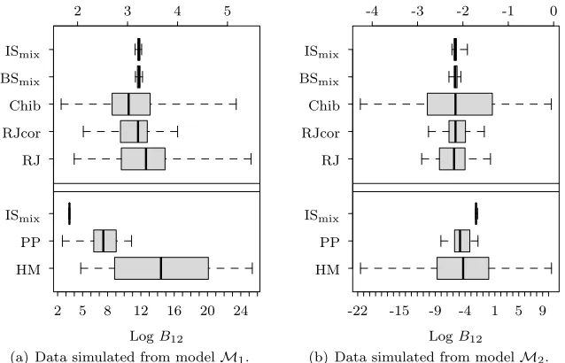
Figure3provides a graphical representation of the variability in log(B12) over
50 repeats of each Monte Carlo approach. The plot highlights that the estimators based on importance sampling and bridge sampling were the most accurate in both scenarios. The left panel of Figure 3 gives results for data generated fromM1. Importance sampling, bridge sampling, Chib and RJ methods lead to
similar estimates, whereas power posterior and harmonic mean overestimated the log Bayes factor. Moreover, RJcor produced slightly more accurate estimates of the log Bayes factor thanvanillaRJMCMC. All methods selected the correct model, with largest variation from the harmonic mean estimator. In the right panel of Figure 3, the results use data generated from model M2. Due to the
huge variance in log(B12), the harmonic mean sometimes favoured the wrong
model. Although the remaining methods correctly identified the true model, the importance and bridge sampling methods again produced the most precise estimates of the Bayes factor; the standard errors provided by the two methods are almost identical.
HM PP ISmix RJ RJcor Chib BSmix ISmix
2 5 8 12 16 20 24
2 3 4 5
LogB12
(a) Data simulated from modelM1.
HM PP ISmix RJ RJcor Chib BSmix ISmix
-22 -15 -9 -4 1 5 9
-4 -3 -2 -1 0
LogB12
(b) Data simulated from modelM2.
Fig 3. Variability of the log Bayes factor estimates based on 50 Monte Carlo repeats for the importance sampling method with mixture proposals (ISmix), bridge sampling method with
mixture proposals (BSmix), Chib’s method (Chib), reversible jump MCMC (RJ), corrected
reversible jump MCMC (RJcor), power posteriors (PP) and harmonic mean (HM) methods (note the different scales for the top and bottom plots).
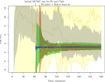
[image:18.612.148.467.367.572.2]M1 as a function of computation time using data generated from M1. The
importance sampling estimator (in blue) converges much more rapidly than the other estimators, showing very tight credible intervals. Chib’s method (in green) and corrected RJMCMC (in red) appear to converge to the same value, but more slowly and have wider CIs. The power posterior method gradually approaches the consensus estimate, requiring significantly more samples to stabilize. The harmonic mean estimator was heavily unstable and also provided much wider credible intervals than the other methods.
0 30 60 90 120 150 180 210 240
Time (minutes)
-2
0
2
4
6
8
10
12
Log
B12
RJ pilot + RJcor burn in Initial MCMC run for IS and Chib
Fig 4. Evolution of log Bayes factor estimates in favour of model M1 as a function of computation time. The solid lines corresponds to the median and the shaded areas give the 95% credible intervals, estimated from 50 Monte Carlo replicates. Yellow represents the harmonic mean method, grey is for the power posterior, red and green correspond to RJMCMC corrected and Chib’s methods respectively and blue represents the importance sampling approach with the mixture proposals.
[image:19.612.139.483.224.493.2]6. Conclusions
In this paper we have introduced a simple three stage algorithm for efficiently es-timating the marginal likelihood. The key components are an MCMC algorithm for obtaining samples from the posterior distribution, π(θ|x), an approximat-ing distributionq(θ) to sample from and an effective estimate of the likelihood π(x|θ). The first observation is whilst an MCMC algorithm will often be rela-tively straightforward to construct, alternative methods for sampling from the posterior distribution could be equally considered. Moreover, it is not impor-tant if a sample from an approximate posterior distribution (for example, Monte Carlo within Metropolis; O’Neillet al., 2000) is used since all that is required for computation of the marginal likelihood is to be able to make a reasonable choice ofq(·). The key limitation to using this approach is effective estimation of the likelihoodπ(x|θ) in cases where it is not analytically tractable. In Section5 of this paper the temporal nature of the data allowed the FFBS algorithm to be utilised to computeπ(x|θ) and more generally filtering methods are a promising avenue of research to explore in the estimation ofπ(x|θ). The importance sam-pling and the associated estimation of the likelihood is trivially parallelisable which can be utilised to speed up implementation. Finally, in cases where the likelihood can easily be computed the algorithm becomes a simple add-on to MCMC to compute the marginal likelihood.
Acknowledgements
PT was supported by a University of Warwick PhD scholarship. NA was sup-ported by a PhD scholarship from the Saudi Arabian Government. PN, SS and TM would like to thank the organisers of the Design and Analysis of Infectious Disease Studies workshop at Oberwolfach (November 2013), where many helpful discussions took place.
We thank an associate editor and a referee for insightful comments which have helped in revising the paper.
References
Addy, C.L., Longini, I.M. and Haber, M. (1991) A generalized stochastic model for the analysis of infectious disease final size data.Biometrics47, 961–974. 10,11
Anderson, B. D. O. and Moore, J. B. (1979) Optimal filtering.Englewood Cliffs, New Jersey: Prentice Hall. 13
Auranen K., Arjas E., Leino T. and Takala A.K. (2000) Transmission of pneum-monococcal carriage in families: a latent Markov process model for binary longitudinal data.J Am Stat Assoc,95, 1044–1053. 12
Carter, C. K. and Kohn, R. (1994) On Gibbs sampling for state space models. Biometrika 81, 541–553. 5,13
Chen, M.-H. (2005) Computing marginal likelihoods from a single MCMC out-put.Statistica Neerlandica59, 16–29. 2
Chib, S. (1995) Marginal likelihood from the Gibbs output.Journal of the Amer-ican Statistical Association90, 1313–1321. 2, 15
Chib, S. and Jeliazkov, I. (2001) Marginal likelihood from the Metropolis-Hastings output.Journal of the American Statistical Association96, 270–281. 2,15
Clancy, D. and ONeill, P. (2007) Exact Bayesian inference and model selection for stochastic models of epidemics among a community of households.Scand. J. Stat.34, 259-274. 11
Clyde, M.A., Berger, J.O., Bullard, F., Ford, E.B., Jefferys, W.H., Luo, R., Paulo, R. and Loredo, T. (2007). Current challenges in Bayesian model choice. In Statistical Challenges in Modern Astronomy IV ASP Conference Series, Vol. 371, proceedings of the conference held 12-15 June 2006 at Pennsylvania State University, in University Park, Pennsylvania, USA. Edited by G. Jogesh Babu and Eric D. Feigelson.p.224. 3
Doucet, A. and Johansen, A. M. (2011) A tutorial on particle filtering and smoothing: fifteen years later. In Handbook of Nonlinear Filtering (eds D. Crisan and B. Rozovsky). Cambridge: Cambridge University Press. pp. 656– 704. 4
Fong, Y., Rue, H. and Wakefield, J. (2010) Bayesian inference for generalized linear mixed models.Biostatistics11, 397–412. 7
Fox, J. P. and Hall, C. E. (1980)Viruses in families.PSG Publishing, Littleton, MA. 10
Friel, N. and Pettitt, A. N. (2008) Marginal likelihood estimation via power pos-teriors.Journal of the Royal Statistical Society: Series B (Statistical Method-ology)70, 589–607. 2,15
Gelfand, A.E. and Dey, D.K. (1994) Bayesian model choice. Exact and asymp-totic calculations.J. Roy. Soc. Series B.56, 501–514. 2,3
Gordon, N.J., Salmond, D.J., and Smith, A.F.M. (1993). Novel approach to nonlinear/non-Gaussian Bayesian state estimation. Radar and Signal Pro-cessing, IEE Proceedings F140, 107-113. 5
Green P.J. (1995). Reversible jump Markov chain Monte Carlo computation and Bayesian model determination.Biometrika82, 711–732. 2,6
Hastings, W. (1970) Monte Carlo sampling methods using Markov chains and their applications.Biometrika,57, 97–109. 2
Hesterberg, T. (1995) Weighted average importance sampling and defense mix-ture distributions.Technometrics,37, 185–194. 4
Hussain M., Melegaro A., Pebody R.G., George R., Edmunds W.J., Talukdar R., Martin S.A., Efstratiou A. and Miller E. (2005) A longitudinal household study ofStreptococcus pneumoniaenasopharyngeal carriage in a UK setting. Epidemiology and Infection 5, 891–898. 12
Statistics22, 623–648. 2
Kass, R.E. and Raftery, A.E. (1995) Bayes factors. Journal of the American Statistical Association.90, 773–795. 2
Kohn, R., Smith, M., Chan D. (2001) Nonparametric regression using linear combinations of basis functions.Statistics and Computing, 11, 313–322. 7 Melegaro, A., Gay, N., and Medley, G. (2004) Estimating the transmission
pa-rameters of pneumococcal carriage in households.Epidemiology and Infection, 132, 433–441. 3,12,15
Metropolis N., Rosenbluth A., Rosenbluth M., Teller A. and Teller E. (1953) Equations of state calculations by fast computing machines.Journal of Chem-ical Physics,21, 1087–1092. 2
Meng, X.-L. and Wong, W. H. (1996) Simulating ratios of normalizing constants via a simple identity: A theoretical exploration.Statistica Sinica,6, 831–860. 2,13,15
Monto, A. S., Koopman, J. S. and Longini, I. M. (1985) Tecumseh study of illness. XIII. Influenza infection and disease, 1976-1981.Amer. J. Epidemiol. 121, 811–822. 10
Neal, P. and Kypraios, T. (2015) Exact Bayesian inference via data augmenta-tion.Stats. and Computing 25, 333–347 10,11
Neal, P. and Subba Rao, T. (2007) MCMC for integer-valued ARMA processes. J. Time Ser. Anal.28, 92–110. 6
Newton, M.A. and Raftery, A.E. (1994) Approximate Bayesian inference with the weighted likelihood bootstrap.J. Roy. Soc. Series B.56, 3–48. 15 O’Neill, P. D., Balding, D. J., Becker, N. G., Eerola, M. and Mollison, D. (2000)
Analyses of infectious disease data from household outbreaks by Markov Chain Monte Carlo methods.J. Roy. Soc. Series C.49, 517–542. 20
O’Neill, P.D. and Marks, P.J. (2005) Bayesian model choice and infection route modelling in an outbreak of Norovirus.Statistics in Medicine24, 2011–2024. Ripley, B.D. (1987).Stochastic Simulation.Wiley & Sons. 3
Roberts, G.O. and Rosenthal, J.S. (2009) Examples of adaptive MCMC.Journal of Computational and Graphical Statistics18, 349–367 14
Skilling, J. (2004) Nested Sampling.AIP Conference Proceedings735, 395-405. 2
Smith, M. and Kohn, R. (1996) Nonparametric regression using Bayesian vari-able selection.Journal of Econometrics, 75, 317–344. 7
Tierney, L. and Kadane, J.B. (1986) Accurate approximations for posterior mo-ments and marginal densities.J. Amer. Stat. Assoc.81, 82–86. 590–599. 3 Zeger, S. (1988) A regression model for time series of counts. Biometrika 75,
621–629. 5,6