Optimal Resource Allocation In
Base Stations for Mobile Wireless
Communications
Zhaoyu Zhong
Management Science
Lancaster University Management School
A thesis submitted for the degree of
Doctor of Philosophy
This thesis is dedicated to Jessica.
Thanks for your company
and
Acknowledgements
I would like to thank both my supervisors: Professor Adam Letchford and Qiang Ni, without whose help I could never have achieved this.
Professor Adam Letchford has been more than helpful throughout my whole PhD life. He helped me in my applications for admission and fundings, he also coached me programming and researching skills. I am so grateful to be one of his students, and words are powerless to express my gratitude.
Professor Qiang Ni brought us an exciting and inspiring topic to work on, based on which the four papers in this thesis were produced.
Papers Arising from the Research
We have included four papers produced during our research in this thesis as listed below. Those papers are presented as Chapters 2-5.
1. A.N. Letchford, Q. Ni & Z. Zhong (2017) An exact algorithm for a resource allocation problem in mobile wireless communications.
Cfomputational Optimization and Applications, 68(2), 193-208. 2. A.N. Letchford, Q. Ni & Z. Zhong (2017) Bi-perspective functions for
mixed-integer fractional programs with indicator variables. Revision submitted to Mathematical Programming
3. A.N. Letchford, Q. Ni & Z. Zhong (2018) A heuristic for maximising energy efficiency in an OFDMA system subject to QoS constraints. In J. Lee, G. Rinaldi & A.R. Mahjoub (eds.) Combinatorial Opti-mization, 303-312. Cham: Springer International Publishing.
4. A.N. Letchford, Q. Ni & Z. Zhong (2018) A Heuristic for Dynamic Resource Allocation in Overloaded OFDMA Systems. Submitted to
Journal of Heuristics
Prof. Qiang Ni contributed the topic of optimisation in OFDMA systems and two classical cases where overall system transmission rate and energy efficiency are maximised respectively. Prof. Adam Letchford made a substantial contribution to all four papers by providing various ideas and mathematical proofs, especially the lemmas, theorems and proofs in the second paper. Inspired by Prof. Letchford, I programmed algorithms and performed experiments to assess all ideas and gave suggestions on modifications of algorithms.
Abstract
Optimal Resource Allocation In Base Stations for Mobile Wireless Communications
Zhaoyu Zhong, B.Sc., M.Sc. PhD thesis, May 2018
Department of Management Science Lancaster University Management School
Telecommunications provides a rich source of interesting and often challenging optimisation problems. This thesis is concerned with a series of mixed-integer non-linear optimisation problems that arise inmobile wireless communications systems.
The problems under consideration arise when mobile base stations have anOrthogonal Frequency-Division Multiple Access (OFDMA)
architecture, where there are subcarriers for data transmission and users with various transmission demands. In such systems, we simultaneously allocate subcarriers to users and power to subcarriers, subject to various constraints including certain quality of service (QoS) constraints called
rate constraints. These problems can be modelled as Mixed Integer Non-linear Programmes (MINLP).
When we began the dissertation, we had the following main aims:
• To design an exact algorithm for the subcarrier and power allocation problem with rate constraints (SPARC), the objective of which is to maximise total data transmission rate of the entire system.
• To design a heuristic algorithm for the F-SPARC problem.
• To design a heuristic algorithm for the SPARC problem in dynamic settings, where user demand changes very frequently.
Contents
1 Introduction 1
1.1 Mobile Wireless Communication . . . 2
1.1.1 Evolution of Multiple Access Schemes . . . 3
1.1.2 Single-user OFDMA systems . . . 6
1.1.3 Multi-user OFDMA systems . . . 7
1.1.4 More complex multi-user problemss . . . 8
1.2 Optimisation . . . 9
1.2.1 Linear programming . . . 9
1.2.2 Non-linear programming . . . 11
1.2.3 Mixed integer linear programming . . . 14
1.2.4 Mixed integer non-linear programming . . . 17
1.2.5 Perspective Function and Perspective Cuts . . . 19
1.3 Research Contribution . . . 22
1.3.1 Research questions . . . 22
1.3.2 Methodology . . . 22
1.3.3 Overview of papers . . . 23
2 An Exact Algorithm for a Resource Allocation Problem in Mobile Wireless Communications 24 2.1 Introduction . . . 24
2.2 Literature Review . . . 25
2.2.1 Single-user systems . . . 25
2.2.2 Multi-user systems . . . 26
2.3 Problem Definition and MINLP Formulations . . . 27
2.3.1 Problem definition . . . 27
2.3.2 Initial convex MINLP formulation . . . 27
2.3.3 Modified convex MINLP formulation . . . 28
2.4.1 A simple outer approximation algorithm . . . 29
2.4.2 Perspective cuts . . . 32
2.4.3 Pre-Emptive Cut Generation . . . 33
2.4.4 Pre-processing . . . 34
2.4.5 Warm-starting . . . 35
2.5 Computational Experiments . . . 36
2.5.1 Test instances . . . 36
2.5.2 Experimental results . . . 37
2.5.3 Comparison with BONMIN . . . 39
2.6 Conclusion . . . 39
3 Bi-Perspective Functions for Mixed-Integer Fractional Programs with Indicator Variables 41 3.1 Introduction . . . 41
3.2 Literature Review . . . 42
3.2.1 Perspective functions . . . 42
3.2.2 Perspective cuts . . . 43
3.2.3 Optimisation in mobile wireless communications . . . 43
3.3 Bi-Perspective Functions and Cuts . . . 44
3.3.1 Bi-P functions . . . 44
3.3.2 Concave envelope . . . 45
3.3.3 Bi-P cuts . . . 47
3.4 Bi-P cuts and Multiple-Choice Constraints . . . 49
3.5 Application to OFDMA Systems . . . 51
3.5.1 The problem . . . 51
3.5.2 Reformulation . . . 52
3.5.3 Bi-P cuts . . . 53
3.6 Computational Experiments . . . 55
3.6.1 Test instances . . . 55
3.6.2 Experimental setup . . . 56
3.6.3 Results . . . 56
4 A Heuristic for Maximising Energy Efficiency in an OFDMA System
Subject to QoS Constraints 59
4.1 Introduction . . . 59
4.2 The Problem . . . 60
4.3 The Heuristic . . . 61
4.3.1 The Basic Idea . . . 62
4.3.2 Improving with Binary Search . . . 63
4.3.3 Improving by Reallocating Power . . . 63
4.4 Computational Experiments . . . 65
4.4.1 Test Instances . . . 65
4.4.2 Results . . . 65
4.5 Concluding Remarks . . . 67
5 A Heuristic for Dynamic Resource Allocation in Overloaded OFDMA Systems 68 5.1 Introduction . . . 68
5.2 Literature Review . . . 70
5.3 A Stochastic Dynamic Version of the SPARC . . . 71
5.3.1 Instance data . . . 71
5.3.2 Objective function . . . 72
5.4 The Heuristic . . . 74
5.4.1 Initial solution . . . 74
5.4.2 Local search . . . 74
5.4.3 Extension to the dynamic case . . . 76
5.5 Experiments . . . 76
5.5.1 Test Instances . . . 76
5.5.2 Results . . . 78
5.6 Conclusion . . . 80
6 Conclusions and Future Work 81 6.1 Summary . . . 81
6.2 Suggestions for Future Work . . . 82
Chapter 1
Introduction
Mobile wireless devices include cell phones, smartphones and tablets. Since the 1980s, when the first generation of mobile wireless networks (1G) was established, the use of such devices has become far more widespread, to the point that they are now an indispensable part of a developed society.
1G networks were unstable, and only voice transmission was possible. 2G net-works brought additional activities such as SMS and browsing text-only webpages. However, 2G networks only allowed data transmission at a peak rate of around 0.5Mbps. These networks pale in comparison to the peak rate of the current 4G net-works which can exceed 300Mbps. Thanks to the rapid evolution in infrastructure, mobile devices are now capable of handling multi-media activities such as live stream-ing. Another recent development is the Internet of Things (IoT), in which everyday devices such as televisions, central heating systems or refrigerators, are connected to the Internet.
As the demand for higher transmission rates continues to climb, access to useful frequency bands in the electromagnetic spectrum (a.k.a. bandwidth) is becoming scarce and expensive. In this context, mathematical optimisation is of critical im-portance for finding improvements in both efficiency and effectiveness of bandwidth use. This is true for long-term (so-called “strategic”), medium-term (“tactical”) and short-term (“operational”) planning (see [64]).
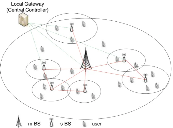
Figure 1.1: Cellular network model.
1.1
Mobile Wireless Communication
In mobile wireless networks, mobile devices (or users) transmit data over carrier waves and are connected to each other by base stations. A base station is a device (or building) with antennae to send and receive calls, texts and multi-media data to and from all devices within its coverage. Mobile phones transmit data to the base station which offers the strongest signal.
The coverage which base stations offer is dependent on many factors such as power supply and graphical characteristics. For best coverage, each base station is assigned a specific coverage area, called acell. A mobile wireless network can be very complicated due to base stations of various sizes and controllers manipulating data transmission between regions. We show a cellular network model in Figure 1.1 with macro base stations (m-BS) and small base stations (s-BS). The cells are represented by small circles.
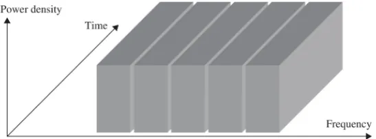
Figure 1.2: Principle of FDMA (with 5 sub-channels)
1.1.1
Evolution of Multiple Access Schemes
Multiplexing is the technology by which voice or data from multiple users can be transmitted on a shared frequency spectrum. Multiple access schemes are the inter-faces applied in mobile networks based on a multiplexing technique. There have been a number of multiple access schemes applied during the history of mobile communi-cations.
1G mobile networks used Frequency-Division Multiple Access(FDMA), which is based on Frequency-Division Multiplexing (FDM). In an FDMA system, data from each user are transmitted via one or several allocated individual sub-channels (see Figure 1.2). Each sub-channel is on a dedicated frequency, and can be only used by one user. In order to prevent interference between sub-channels, there are gaps between each pair of sub-channels. These are called guard bands. Despite FDMA having advantages such as simple implementation, its disadvantages far outweigh them. Guard bands between sub-channels, used to avoid interference, result in a waste of spectrum. Furthermore, the quality of transmission in 1G analogue networks was not guaranteed when users were physically close to each other. FMDA soon became redundant in mobile wireless communications.
The second generation of mobile wireless communications transited from ana-logue to digital technology. Time-Division Multiple Access (TDMA), a scheme based onTime-Division Multiplexing (TDM), was applied in 2G networks enabling simple data transmission services. In TDMA systems, data of all users are transmitted over the same frequency but in individual short time slots. In each time slot, the data of only one user can be transmitted (see Figure 1.3. TDMA allowed transmission of data from multiple users on the same frequency, but not simultaneously.
Code-Division Multiple Access (CDMA), based on Code-Division Multiplexing
main-Figure 1.3: Principle of TDMA (with 5 time-slots)
Figure 1.4: Principle of CDMA (with 5 spreading codes)
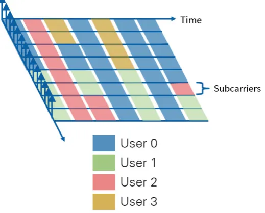
[image:13.595.187.437.314.409.2] [image:13.595.179.443.496.702.2]Figure 1.6: OFDMA subcarriers allocation over time
stream during the 3G era. CDMA enables data of more than one user to be trans-mitted on the same frequency, at the same time, by allocating a random spreading code to each user (see Figure 1.4). In a CDMA network, data from all users are transmitted at the same rate. This is not an optimal solution due to users having varying demands.
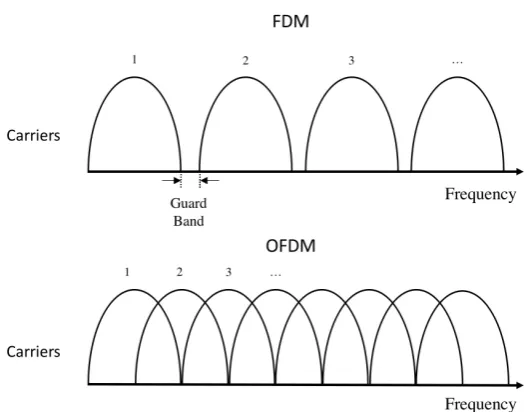
As the demand for higher data transmission rate increased, the Orthogonal Frequency-Division Multiplexing (OFDM) technique was proposed. OFDM is based on FDM. However, a frequency is divided into many orthogonal carriers to carry an information stream. All carriers are orthogonal to one another to avoid inter-ference, so on a fixed bandwidth there can be more carriers than FDM carriers for data transmission (see Figure 1.5). Meanwhile, the orthogonal distribution of carriers eliminated guard bands between FDM carriers for interference prevention.
Orthogonal Frequency-Division Multiple Access(OFDMA) is an accessing scheme based on the OFDM technique, and is widely applied in the current 4G Long Term Evolution(LTE) networks. It is the multi-user version of OFDM. By further dividing carriers into subcarriers and allocating subcarriers to different users, multiple access is achieved. While OFDMA may assign an individual user more than one subcarrier, a subcarrier can only be assigned to one single user. The allocation will vary depending on the number of users in the system, and the demand of each user.
the two users left the system in the next time slot and all subcarriers were allocated to User 2. The adaptive subcarrier allocation in OFDMA systems is recognised as an efficient multiple access approach for wireless networks.
All four papers in this thesis are based on the OFDMA scheme. The subcarrier and power allocation problem in OFDMA systems will be introduced in subsection 1.1.2–1.1.4.
1.1.2
Single-user OFDMA systems
Data are transmitted over subcarriers in OFDMA networks and there are many factors which affect the transmission rate. The commonly known Shannon-Hartley theorem in information theory tells the capacity of a subcarrier (i.e. theoretical maximum bit-rate that can be transmitted, see [45]) given its bandwidth and noise. It states that:
C =B log2(1 + p
N) bits/second, (1.1)
where C is subcarrier capacity, B is subcarrier bandwidth measured in Hertz, p is power in Watts supplied to the subcarrier andN is noise in Watts on that subcarrier. For a given subcarrier, its bandwidth B is usually a known constant. Noise on subcarriers varies from time to time, but for simplification we use the average noise of that subcarrier, so that we will have a non-linear function of C against p.
Consider an OFDMA system where there is one user and a set|I|of subcarriers, and each subcarrier i ∈ I has its own bandwidth Bi and noise power Ni. If we
allocate pi watts of power to subcarrier i, the data rate for that subcarrier will be
Bilog2(1 +pi/Ni), which we denote byfi(pi). A natural optimisation problem is then
to maximise the total data rate subject to an overall power limit P. This can be formulated as the following NLP:
max
i∈I
fi(pi) :
i∈I
pi ≤P, p∈R|+I|
. (1.2)
Since the functions fi(pi) are concave, this NLP can be solved efficiently by any
non-full containers at a constant rate. From a formal point of view, water-filling can be regarded as a variant of the steepest-ascent (a.k.a. gradient or hill-climbing) method. For brevity, we do not introduce details of the algorithm, but one can find a comprehensive example at [1].
1.1.3
Multi-user OFDMA systems
As mentioned in subsection 1.1.1, OFDMA systems are multi-user systems, and each subcarrier can be assigned to an arbitrary user. Now we discuss problem 1.2 in a multi-user scenario.
Suppose we have subcarrier set I and user set J, a bandwidth Bi >0 and noise
Ni >0 for each i ∈ I, and a power limit P > 0. The task is to allocate subcarriers
to users, and power to subcarriers, in order to maximise the total data rate, subject to a constraint stating that the total power must not exceedP.
We formulate the problem as an MINLP (see 1.2.4 for an introduction). For all i∈I and j ∈J, letxij be a binary variable, taking the value 1 if and only if user j is
assigned to subcarrier i. Also let pij be a continuous variable, taking the value zero
if xij = 0, but otherwise representing the amount of power supplied to subcarrier i.
We then have:
max i∈Ij∈Jfi(pij) (1.3)
s.t. i∈Ij∈Jpij ≤P (1.4)
j∈Jxij ≤1 (∀i∈I) (1.5)
pij ≤P xij (∀i∈I, j ∈J) (1.6)
pij ∈R+ (∀i∈I, j ∈J) (1.7) xij ∈{0,1} (∀i∈I, j ∈J). (1.8)
The objective function (1.3) represents the total data rate. The constraint (1.4) imposes the power limit. The constraints (1.5) ensure that each subcarrier is allocated to one user at most. The constraints (1.6), called variable upper bounds (VUBs), ensure that pij is zero whenever xij is zero. The remaining constraints are the usual
non-negativity and binary conditions.
1.1.4
More complex multi-user problemss
The first problem that we focus on in this thesis is that of simultaneously allocating subcarriers to users and power to subcarriers, subject to certain quality of service (QoS) constraints called rate constraints, in order to maximise the total data trans-mission rate. We call this problem the subcarrier and power allocation problem with rate constraints (SPARC) problem.
If we let J denote the set of users, then the total data rate for that user will be i∈Ifi(pi). The constraint 1.6 ensures that pij = 0 when i /∈ Sj, therefore
i∈I fi(pi) = i∈Sjfi(pi). We add an extra constraint to the multi-user OFDMA
problem so that data rate for user j should be at least the demand of user j, which we denote byℓj:
i∈I
fi(pij)≥ℓj (∀j ∈J). (1.9)
There are many papers on such optimisation problems in OFDMA systems. Wong & Cheng [82] minimise total power subject to individual quality of service (QoS) constraints that impose a lower bound on the data rate for each user. Rhee & Cioffi[65] achieve QoS in a different way, by maximising the minimum data rate over all users, subject to a limit on total power. Kim et al. [41] consider the problem of maximising total data rate subject to a total power limit. Shenet al.[73] add a global QoS constraint to that problem. Seung et al. [70] enforce QoS by giving each user a weight, and maximising a weighted sum of the data rates. Yu & Lui [87] consider an extension of the problem in [70], in which there is interference between channels. Tao et al. [76] take the problem in [41], add rate constraints, and also consider an extension in which transmissions can suffer delays.
More recently, perhaps driven by environmental considerations, authors have focused on maximising energy efficiency, which is defined as total data rate divided by total power (e.g., [23, 34, 79, 84, 85, 88]). Therefore, the second problem we will introduce in this thesis is thefractional subcarrier and power allocation problem with rate constraints (F-SPARC) problem, continuing this trend. The F-SPARC problem is very similar to the SPARC problem, but with objective function being maximising
energy efficiency, which is defined as total data rate divided by total power supplied to the system:
max
i∈I
j∈Jfi(pij)
σ+i∈Ij∈Jpij
. (1.10)
areN P-hard in the strong sense as well. However, the function fi is concave over the
domain [0, P] for alli ∈I. As a result, the objective function (1.3) is concave. This means that the problem is convex, therefore, its continuous relaxation can be solved efficiently via convex programming techniques.
1.2
Optimisation
Optimisation, also known asmathematical programming, is a discipline branched from applied mathematics, the goal of which is finding the best solutions for real-world problems using mathematical tools.
Optimisation has been widely applied in a number of fields including transporta-tion, manufacturing, inventory control, scheduling, and networking. Developments in telecommunications has also provided a rich source of optimisation problems, includ-ing our SPARC and F-SPARC problems (see [64]).
A typical optimisation problem often consists of an objective function, variables
and variousconstraints. Solving an optimisation problem means finding values of the variables that maximise or minimise the objective function, subject to all constraints. A basic optimisation problem takes the form
max f0(x)
s.t. fi(x)≤0 i={1, ..., m},
x∈X
(1.11)
where x is the variable vector, X is the domain of the variables (continuous, inte-ger, binary, or some mixture), function f0 : Rn → R is the objective function, and functions fi : Rn → R, i = {1, ..., m} are the constraints. A solution is feasible if
it satisfies all m of the constraints, and the area formed by all feasible solutions is called the feasible region. If the problem is to minimise the objective function, one can easily multiply the objective function by −1. Equation constraints can also be added to an optimisation problem, but they are not covered in this thesis.
In this section, we will introduce common optimisation problems involved in this paper.
1.2.1
Linear programming
❜❜ ❜❜ ❜❜❜❜ ❆ ❆ ❆ ❆❆ ✻ ✲ x 1 x2
*
1 2 3 [image:19.595.242.389.112.255.2]1 2 3
Figure 1.7: Feasible region of LP example bounded by five constraints
max cTx
s.t. Ax ≤ b x ≥ 0,
(1.12)
whereAis a matrix of constants, candb are column vectors,xis the variable vector, b and c are vectors of given coefficients.
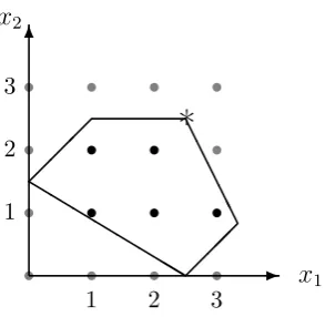
We show an example of a maximisation LP problem here with its feasible region plotted on a 2D graph shown in figure 1.7:
max x1 + x2
s.t. −2x1 + 2x2 ≤ 3 2x1 − 2x2 ≤ 5 −6x1 − 10x2 ≤ −15
2x2 ≤ 5 4x1 + 2x2 ≤ 15
x1, x2 ≥ 0
(1.13)
It is proven in [60] that if a linear programming problem has one or more points which maximises (or minimises in minimisation problems) the objective function, then at least one of those points is the extreme point. It is also shown that if an extreme point is not the optimal solution, there must be an edge which has a better solution on the other side connected to this point. Solutions on extreme points are called corner point solutions. In the case of problem (1.13), the corner point solutions are {(0,1.5),(1,2.5),(2.5,0),(31,56),(2.5,2.5)}, and the optimal solution is (2.5,2.5). A very effective algorithm called thesimplex methodwas proposed by Dantzig in 1947 to solve linear programming problems by searching corner point solutions.
is not, then it searches all edges connected to this point to find the one which offers the best corner point solution and moves to that extreme point. The algorithm stops once the optimal solution has been found.
Unfortunately, simplex method is not a polynomial-time algorithm (see [43]), and can encounter difficulties when solving large-scale LP problems. A few techniques has been proposed for those LPs.
Benders decomposition, also known as row generation, is a technique for solving LP problems with block structures (see [4,14]). Firstly, it divides all variables into two subsets, and solves a master problem based on one subset of variables. Some variable values of the optimal solution from this stage will be fixed and a sub-problem will be formulated with the other subset of variables. For those given fixed variable values, if the subproblem is infeasible, Benders cut will be added to be master problem in order to reduce searching space. The process will continue until no Benders cuts can be generated.
Column generation is another technique widely used to solve LP problems with a large number of variables (see [14]). A master problem is derived from the original problem and only considers a subset of variables. A subproblem is then created to identify a new variable to add to the master problem, utilising reduced cost in duality theory. The algorithm keeps adding new variables when its reduced cost is negative and will stop when no variables can be added to the master problem.
Several other algorithms have been proven to run in polynomial time (e.g., Khatchian’s ellipsoid method in [40], and the Karmarkar’s projective method in [36]). Therefore, in computational complexity theory, LP problems are classified asP prob-lems, which means they can be solved in polynomial time, such that the time to solve the problem increases as a polynomial function as the size of the input increases. An LP problem of reasonable scale is often easy to solve by most solvers available.
1.2.2
Non-linear programming
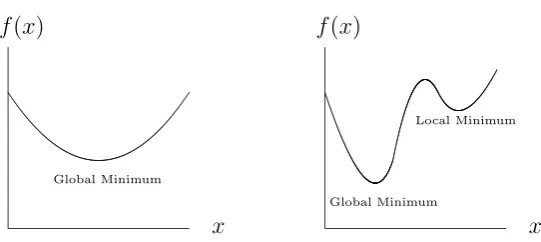
In contrast to linear programming, a problem is a non-linear programming (NLP) problem if the objective function or any of the constraints in problem (1.11) is not linear.
x f(x)
x f(x)
Global Minimum
Global Minimum
[image:21.595.183.454.108.229.2]Local Minimum
Figure 1.8: A convex function (left) and a non-convex one (right)
the most difficult N P problems (N P-complete problems). Although not yet proven, it is widely believed that there are no polynomial-time algorithms for N P-complete problems.
One important type of NLP optimisation problem is the convex optimisation
problem. While convex optimisation is now a somewhat mature technique, it has been proven in [61] that a non-linear programme with a non-convex quadratic function is
N P-hard even when the only constraints present are non-negativity constraints. We now present definitions related to convex optimisation before we can explain further.
Definition 1 A function f :X →R is convex if:
ftx1+ (1−t)x2 ≤tf(x1) + (1−t)f(x2) ∀x∈X,∀t ∈[0,1].
Definition 2 A function f :X →R is concave if -f is convex.
Definition 3 A set C is convex if for any two points x1, x2 ∈C and any θ in [0,1], we have:
θx1+ (1−θ)x2 ∈C.
Definition 4 A problem is a convex optimisation problem if it takes the form (1.11)
and functions fi, i={0, ..., m} are all convex functions.
Definition 5 A point x∗ is a global maximum of f if f(x∗)≥f(x) ∀x∈S, where S
is the feasible region.
x f(x)
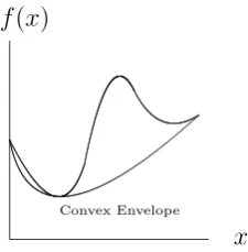
[image:22.595.262.375.113.228.2]Convex Envelope
Figure 1.9: Convex envelope of a non-convex function
over the whole feasible region, whereas local optima are the best solutions among a subset of the feasible region. Therefore, when minimising a non-convex objective functionf, one can utilise a convex function which underestimates or equalsf in the same domain. The convex function is the convex envelope of the non-convex function f. On the other hand, concave envelopes are applicable in maximisation problems (see Figure 1.9).
An Outer approximation (OA) algorithm was designed for convex NLPs, pro-posed by Kelley (see [38]) in 1960s. Suppose we have a convex NLP of the following form:
maxf(y) : y∈C ⊆Rn
+
, (1.14)
wheref(y) is a convex non-linear function of the decision variable vector y, and
C is the domain of y.
The problem can be reformulated into:
maxz : z ≤f(y), z∈R, y ∈C ⊆Rn+
(1.15)
by introducing an extra continuous variablez.
The key idea of Kelley’s algorithm is to approximate the convex constraint with a collection of linear constraints of the form:
z ≤ f(¯y) +f′(¯y)y − y¯, (1.16) where f′ denotes the first derivative of f. The constraints (1.16) are called Kelley
cuts. By approximating all non-linear constraints with Kelley cuts, the problem is then an LP relaxation of the original NLP. The algorithm converges to a solution with acceptable optimality gap when more and more Kelley cuts are added.
1.2.3
Mixed integer linear programming
In real life there are always problems whereby solution spaces are discrete rather than continuous. Problems of this type are calleddiscrete optimisation which usually, but not necessarily, involves integral variables. A particularly important application of discrete optimisation is to model and solvecombinatorial optimisation problems (see [44]). These are optimisation problems that involving concepts from combinatorics (such as sets, subsets, combinations and permutations) and graph theory (such as nodes, edges, cliques, cuts and flows).
Mostcombinatorial optimisationproblems can be modelled asMixed integer pro-grammings(MIPs) orMixed integer linear programmings(MILPs),in which some vari-ables can only take integral values. MILP is itself a subset of discrete optimisation, and takes the form of
max cTx + dTy
s.t. Ax + Ey ≤ b x, y ≥ 0
y ∈ Z.
(1.17)
When x is an empty set, i.e., all variables are required to be integers, the prob-lem is often called integer programming (IP). For brevity, we mention both types of programmes as MIP below.
A special case of an MIP problem is called binary integer programming, where some, or all, integral variables can only take the value 0 or 1. A binary variable is often considered as a ”yes-or-no” variable: it takes value 1 when the answer is ”yes” and 0 for ”no”.
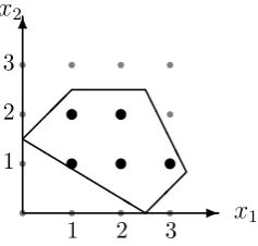
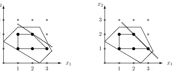
We continue using the LP example in subsection 1.2.1 with an extra constraint that bothx1 and x2 are integers, so it becomes an IP problem. The feasible region of the problem is then discrete due to the new integral constraint. As shown in Figure 1.10 as black dots, there are five integral solutions bounded by the five constraints.
Although MIP is similar in form to LP, the involvement of integrity of variables makes the difficulty of an optimisation problem increase exponentially. IP problems are proven to beN P-hard in general (see [37]). Since MILP problems are even more general than ILP, they also tend to be N P-hard. Many efforts have been made to solve MIP problems, and we will introduce some of the most successful algorithms in the remaining part of this subsection.
❜❜ ❜❜ ❜❜ ❆ ❆ ❆ ❆ ✻ ✲ x1 x2 1 2 3
[image:24.595.256.375.113.226.2]1 2 3
Figure 1.10: Feasible region of IP example bounded by five constraints
✉ ✉ ✉ ✉ ✉ ❜❜ ❜❜ ❜❜❜❜ ❆ ❆ ❆ ❆ ❆ ✻ ✲ x1 x2
*
1 2 31 2 3
✉ ✉ ✉ ✉ ✉ ❜❜ ❜❜ ❜❜❜❜ ❆ ❆ ❆ ✻ ✲ x1 x2
*
1 2 31 2 3
Figure 1.11: Cutting plane method for integer programming
new linear, non-redundant constraints to the original problem in order to reduce the size of the feasible region.
Geometrically, a cutting plane is a hyperplane which separates all MIP feasible solutions on one of its sides (see Figure 1.11). A cutting plane (or cut) is only valid if it eliminates some of the feasible region and is satisfied by all feasible solutions of the original MIP problem.
By keeping added cutting planes, the optimal integral solution will eventually become an extreme point and can be obtained by solving the relaxation problem. It is then critical to find strong cutting planes in order to cut off as much as possible. We show two types of strong cuts in Figure 1.12. The cutting plane on the left touches the polyhedron formed by all integral solutions, while the one on the right defines a facet of the polyhedron and is the strongest possible cutting plane.
[image:24.595.145.490.282.424.2]✉ ✉ ✉ ✉ ✉ ❅ ❅ ❅ ❜❜ ❜❜ ❜❜❜❜ ❆ ❆ ❆ ❆ ❆ ✻ ✲ x 1 x2 1 2 3
1 2 3
✉ ✉ ✉ ✉ ✉ ❜❜ ❜❜ ❜❜❜❜ ❆ ❆ ❆ ❆ ❆ ❅ ❅ ❅ ✻ ✲ x 1 x2 1 2 3
[image:25.595.149.490.112.260.2]1 2 3
Figure 1.12: Strong cutting plane method for integer programming
Another successful method is thebranch and bound(BB) method (see [46]). The branch and bound method partitions the solution space of a problem into a tree structure, and explores the solution space node by node until it finds the optimal solution.
First, the branch and bound algorithm solves the relaxation of the original MIP maximisation problem to get an upper bound, it then obtains a lower bound based on the relaxed solution. Take the IP problem as an example, we know from subsection 1.2.1 that the optimal objective value is 5 whenx1 =x2 = 2.5. However, this solution is fractional, thus infeasible. However, the relaxed optimal value can be used as an upper bound, since no solution of the original problem can yield an objective value higher than 5. We can then round-down the two variables to 2, in order to obtain a lower bound of this problem.
The algorithm then partitions the solution space based on a variable by gen-erating two sub-problems. Suppose we choose variable x1 to partition the solution space. We get two natural sub-problems, in each of which there exists an additional constraint. In one of the sub-problems, the additional constraint is x1−2 ≤ 0; the one in the other sub-problem is x1 −3 ≥ 0. The two sub-problems are presented in Figure 1.2.3. By solving the first sub-problem, we get a relaxed optimal solution (2,2.5). In the second sub-problem, the relaxed optimal solution is (3,1.5).
✉ ✉ ✉ ✉ ❜❜ ❜❜ ❜❜ ✻ ✲ x 1 x2
*
1 2 31 2 3
✉ ❆ ❆ ✻ ✲ x 1 x2
*
1 2 31 2 3
The branch and bound method is intelligent in four aspects:
1. The enumeration process stops when optimal solution is found
2. It recognises solution space where no optimal solution exists
3. It recognises solution space where no feasible solution exists
4. It searches the most promising solution space first
The branch and bound method is an exact algorithm which means it is guaran-teed to find the optimal solution. However, it is an enumeration algorithm, it needs to solve a huge number of sub-problems when facing complex problems, and that can cause memory and time issues.
We remark that both Bendess Decomposition and Column Generation can be applied to MILPs. By combining those algorithms with B&B, branch and cut (see [62]) and branch and price (see [2]) are proposed and widely used for solving large MILPs.
1.2.4
Mixed integer non-linear programming
The most difficult class of optimisation problem is formed by the mixed integer non-linear programming problems (MINLP), which take the form
min f(x, y)
s.t. c(x, y) ≤ 0
x ∈ R
y ∈ Z
(1.18)
MINLP are optimisation problems which consist of both non-linear elements (objective function and/or constraints) and integral variables. As a result, most MINLP problems areN P-hard.
Solving an MINLP problem is usually very challenging due to the fact that it combines the difficulties from both NLP and MIP problems. We now introduce some of the algorithms available for MINLP problems.
1. Branch and bound can also be applied to MINLPs. The non-linear BB method solves an NLP instead of an LP relaxation problem during its iterative routine, it does not differ greatly from the linear BB method. However, as mentioned in subsection 1.2.3, the BB algorithm is not efficient when there are too many sub-problems to solve.
2. Outer Approximation algorithms can also be used to solve convex MINLP prob-lems. By solving two sub-problems derived from the original MINLP problem, the OA method obtains an upper bound and a lower bound. An MILP master problem is then formulated, and cutting planes are added to it based on the relaxation solution obtained from one of the sub-problems. The MILP master problem is a relaxation of the original MINLP problem, but by adding cutting planes effectively, it will approximate the non-linear feasible region and update bounds in every iteration. The OA algorithm stops when the difference of the two bounds becomes smaller than some criterion. Indeed, Kelley’s cuts can be integrated with Gomory’s cuts to solve convex MINLPs.
3. Generalised Benders decomposition(GBD) is generalised from the Benders de-composition method to solve convex MINLP problems. The GBD method does not require sub-problems to be linear, but some issues have been found: in some cases it may only converge to a local minima, in other cases it may not converge at all.
f
x
[image:28.595.167.455.111.296.2]t
Figure 1.13: Example of a perspective function
MINLP problems are extremely difficult to solve. The OA, GBD and LP/NLP based BB methods are all for convex MINLP problems only. For non-convex MINLP problem, a comprehensive list of solvers can be found at [57]. There are some good surveys available for both convex and non-convex MINLP problems, see [6, 9, 13, 19, 25, 29, 51].
1.2.5
Perspective Function and Perspective Cuts
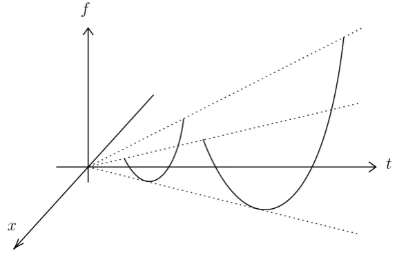
A very importance concept we will use in this thesis is the perspective function (see [31]). The perspective of a functionf :Rn→Ris the function g :Rn+1 →R, defined byg(x, t) = tf(x/t). By definition, the perspective function g takes the value 0 when t= 0. The perspective operation of a function preserves convexity (concavity) of the original function f.
Obviously, the perspective function g is equivalent to the original function f when t = 1. We show the perspective of f in Figure 1.13. One can see that the variablet only scales the functionf but has not effect on its shape.
One of the important applications of perspective functions is to solve fractional programs, which takes the form:
maxf(y)/g(y) : x∈C,
where C ⊆ Rn is convex, f(y) is non-negative and concave over the domain C, and
g(y) is positive and convex over the domainC. It is shown in [10,69] that by utilising perspective function, such a problem can be reformulated as
z
x
y
z
x
y
0 0
[image:29.595.103.527.102.291.2]1 1
Figure 1.14: Perspective cuts of a nonlinear function with an indicator variable
where t is a new non-negative variable representing 1/g(y), and y′ is a new vector of variables representingy/g(y). The reformulated problem can often be solved effi-ciently, since the objective function is concave and the feasible region is convex.
Frangione & Gentile also showed that perspective functions can be used to gen-erate stronger cutting planes when solving MINLPs with indicator variables.
We now introduce an indicator variablexto the problem (1.14) so that if xtakes the value zero, then all of the components of y must also take the value zero. The problem then becomes an MINLP as following:
maxf(y) : yj ≤M x, x∈{0,1}, yj ∈C ⊆Rn+ ∀j ∈{1, ..., n}
, (1.19)
whereM is the largest values y can take.
The continuous relaxation of the convex MINLP is strengthened if we replace the functionf(y) with theperspective function xf(y/x). The effect of this strengthening on an OA algorithm is as follows. Let z be a continuous variable representing the functionf(y), and let
z ≥f(¯y) +∇f(¯y)·(y−y)¯
be the associated Kelley cuts. Letting z represent the perspective function xf(y/x) instead, the Kelley cuts change to:
z ≥ ∇f(¯y)·y+f(¯y)− ∇f(¯y)·y¯x.
Geometrically, the original Kelley cuts are a collection of planes over the feasible region of the NLP relaxation of problem (1.19), whereas the strengthened ones are planes cutting thought that feasible region connecting the non-linear function f and the grid origin so that the non-linear functionf is projected into a point as xreduces from 1 to 0 (see Figure 1.14). The strengthened cuts are very helpful when solving the MILP or even LP relaxation of problem (1.19).
When dealing with afractional program with indicator variables, we found that, in order to obtain tight convex relaxations of such problems, perspective cuts can also be applied, but one needs to study a new kind of function, which we call a
bi-perspective (Bi-P) function.
Letybe a vector of ncontinuous variables, letf(y) be a real function ofythat is defined over a convex domain C ⊆Rn
+, and let t1 and t2 be non-negative continuous variables. The Bi-P function off(y) is defined as:
t1t2f
y t1t2
,
with domain t1, t2 ∈ R+, y ∈ t1t2C. (By convention, the Bi-P function takes the value zero when t1t2 = 0 andy is the origin.)
Whereas standard perspective functions preserve convexity and/or concavity, the same is not true for Bi-P functions. So we need to obtain the concave envelope of the Bi-P function as follows.
Define the following two auxiliary functions:
g1(t1, t2) = a2t1+b1(t2−a2) g2(t1, t2) = a1t2+b2(t1−a1).
We prove in Chapter 3 that the concave envelope, over the domain t1 ∈ [a1, b1], t2 ∈[a2, b2] andy ∈t1t2C, is:
min
g1(t 1, t2)f
y g1(t1, t2)
, g2(t 1, t2)f
y g2(t1, t2)
. (1.20)
We then obtain the hypograph of the function (1.20) described by the linear inequalities
z ≤ ∇f(¯y)y + f(¯y)− ∇f(¯y) ¯ygkt1, t2 (1.21) for ¯y ∈C and k = 1,2. We call the inequalities the Bi-P cuts.
We remark that when t2 is an indicator variable, the Bi-P cuts reduce to:
1.3
Research Contribution
1.3.1
Research questions
As mentioned in subsection 1.1.4, a lot of the SPARC problem variants considered in the cited papers areN P-hard in the strong sense. Accordingly, in all of the those papers, the authors use relaxation techniques to compute bounds, and heuristics to find feasible solutions. An issue arises in whether we can solve the SPARC problems exactly using MINLP.
While exact algorithms put emphasis on optimality, we are also concerned with heuristics that can solve SPARC problems both effectively and efficiently in realistic scenarios. Moreover, we are also interested in a heuristic for dynamic and overloaded systems, where total user demand changes frequently and is sometimes higher than system capacity.
1.3.2
Methodology
As a kind of natural science, optimisation has had a somewhat standardised method-ology since its inception in the 1950s when researchers started Operational Research. Since then, the methodology used for optimisation has remained largely unchanged. Approaches for optimisation follow specific steps, and for each step there corresponds a specific methodology. Almost all researches in optimisation follow the specific steps presented in this subsection.
1. Understanding and describing problem
2. Building a mathematical model
3. Development and refinement of the model
4. Algorithm design
5. Algorithmic complexity analysis
6. Coding and debugging
7. Design of test instances
8. Computational experiments
1.3.3
Overview of papers
We now present the structure of this thesis in this subsection.
In Chapter 2, we will introduce the SPARC problem and its variants in subsec-tion 2.3. We will then present an exact algorithm in subsecsubsec-tion 2.4, which uses a combination of outer approximation [18] and perspective cuts [22, 26], together with three implementation “tricks” of our own, which improve the running time by several orders of magnitude. Computational experiment results given in subsection 2.5 show that our algorithm is capable of solving SPARC problem instances of realistic size and complexity, to proven optimality, in about one minute.
Following on, we will introduce an exact algorithm for the F–SPARC problem in Chapter 3. In subsection 3.3, we will define bi–perspective (BP) function and char-acterise the concave envelope of a BP function over a rectangular domain. We then derive a family of linear inequalities, which we callBP cuts, that completely describe the concave envelope. In subsection 3.4, we will demonstrate how to generalise the BP cuts when there are “multiple-choice” constraints, stating that two or more indicator variables cannot take the value 1 simultaneously. Computational experiment results in subsection 3.6 show that the new cuts typically close over 95% of the integrality gap.
In Chapter 4, we will present a heuristic algorithm which solves the same problem as in Chapter 3. We then consider the SPARC problem in dynamic and overloaded cases in Chapter 5. In subsection 5.3.2 we introduce an objective function which takes fairness into consideration. A dynamic local search heuristic is then proposed in subsection 5.4.
Chapter 2
An Exact Algorithm for a
Resource Allocation Problem in
Mobile Wireless Communications
2.1
Introduction
Telecommunications provides a rich source of interesting, and often challenging, opti-misation problems (see, e.g., Resende & Pardalos [64]). This paper is concerned with a mixed-integer convex optimisation problem that arises in mobile wireless commu-nications systems. In such systems, mobile devices (such as smartphones or tablets) communicate with one another via transceivers called base stations. Each base sta-tion must periodically allocate its available resources (time, power and bandwidth) in order to receive and transmit data in an efficient way (see, e.g., Fazel & Kaiser [17]). The problem under consideration arises when the base stations have an Orthogo-nal Frequency-Division Multiple Access (OFDMA) architecture. This means that the base station divides the available bandwidth into a number of frequency bands called
subcarriers. Each subcarrier can be assigned to only one mobile device (or user) in any given time period, but a given user may be assigned to more than one subcarrier. The data transmission rate for any given subcarrier is a nonlinear function of the power allocated to that subcarrier.
subcarrier and power allocation problem with rate constraints(SPARC).
The SPARC has a natural formulation as a convex mixed-integer nonlinear pro-gram (MINLP). Since we found that standard software for convex MINLP was un-able to solve even small instances of our problem in reasonun-able computing times, we developed our own specialised exact algorithm. It uses a combination of outer approximation [18] and perspective cuts [22, 26], together with three implementation “tricks” of our own, which improve the running time by several orders of magnitude. A novel ingredient of our algorithm, which turned out to be crucial, is what we callpre-emptive cut generation. By this, we mean the generation of cutting planes that are not violated in the current iteration, but are likely to be violated in subsequent iterations.
It turns out that our exact algorithm is capable of solving SPARC instances of realistic size and complexity to proven optimality in about one minute. In fact, instances with relatively loose QoS constraints can be solved in a fraction of a second. As far as we know, our algorithm is the first viable exact algorithm for a realistic OFDMA optimisation problem. It is also the first algorithm to apply perspective cuts to a problem in mobile wireless communications.
The paper is structured as follows. The relevant literature is reviewed in Section 2.2. In Section 2.3, we define the SPARC formally and present a convex MINLP formulation for it. The exact algorithm is described in Section 2.4. The results of some extensive computational experiments are given in Section 2.5, and some concluding remarks are made in Section 2.6.
We assume throughout that the reader is familiar with basic concepts of MINLP, such as continuous relaxation, convexity, lower and upper bounds, and branching. For tutorials, see, e.g., [3, 13, 81].
2.2
Literature Review
Now we briefly review the literature on optimisation in OFDMA and related systems. Good reference texts are [12, 17, 27].
2.2.1
Single-user systems
First, consider a single communications channel and a single user. The classical
Shannon–Hartley theorem [71] states that the maximum data rate (in bits per second) that can be transmitted from a single channel is:
where B is the bandwidth of the channel in Hertz, S is the average received signal power in watts, and N is the average noise power in watts. The quantity S/N is called the signal-to-noise ratio.
Now suppose that we still have a single user, but we now have a set I of sub-carriers, and each subcarrier i∈ I has its own bandwidth Bi and noise power Ni. If
we allocate pi watts of power to subcarrier i, the data rate for that subcarrier will
be Bilog2(1 +pi/Ni), which we denote by fi(pi). A natural optimisation problem is
then to maximise the total data rate subject to an overall power limit P. This can be formulated as the following NLP:
max
i∈I
fi(pi) :
i∈I
pi ≤P, p∈R|+I|
. (2.1)
Since the functions fi(pi) are concave, this NLP can be solved efficiently by any
standard technique for convex optimisation (see, e.g., Boyd & Vandenberghe [8]). It can also be solved quickly by a specialised iterative technique calledwater filling; see, e.g., [12, 27].
2.2.2
Multi-user systems
As mentioned in the introduction, OFDMA systems are multi-user systems, and each subcarrier can be assigned to an arbitrary user. If we let J denote the set of users, and Sj ⊂ I denote the set of subcarriers allocated to user j ∈ J, then the total
data rate for that user will be i∈Sjfi(pi), and the total data rate for the system
will be j∈Ji∈Sjfi(pi). One then faces optimisation problems in which one must
simultaneously distribute the available power between the subcarriers, and allocate each subcarrier to a user, in order to meet some objective.
More recently, perhaps driven by environmental considerations, authors have focused on maximising energy efficiency, which is defined as total data rate divided by total power (e.g., [23, 34, 79, 84, 85, 88]).
It is proved in [52,53] that many of the problem variants considered in the above papers areN P-hard in the strong sense. Accordingly, in all of the above-mentioned papers, the authors use relaxation techniques to compute bounds, and heuristics to find feasible solutions. In this paper, we focus on exact methods.
2.3
Problem Definition and MINLP Formulations
We now formally describe the problem under consideration and give two MINLP formulations of it.
2.3.1
Problem definition
Although the methods developed in this paper can be applied to several OFDMA optimisation problems, we restrict attention to one specific problem, for the sake of brevity and clarity. As mentioned in the introduction, we call this problem the SPARC. A SPARC instance is given by sets I and J, a bandwidthBi >0 and noise
Ni > 0 for each i ∈ I, a user rate ℓj ≥ 0 for each j ∈ J, and a power limit P > 0.
As in [41, 73], the task is to allocate subcarriers to users, and power to subcarriers, in order to maximise the total data rate, subject to a constraint stating that the total power must not exceed P. In addition, however, we have rate constraints, as in [76,82], stating that the total data rate for userj must be at leastℓj. We conjecture
that the SPARC is N P-hard in the strong sense.
2.3.2
Initial convex MINLP formulation
We formulate the SPARC as an MINLP as follows. For alli∈I and j ∈J, letxij be
representing the amount of power supplied to subcarrieri. We then have:
max i∈Ij∈Jfi(pij) (2.2)
s.t. i∈Ij∈Jpij ≤P (2.3)
j∈Jxij ≤1 (∀i∈I) (2.4)
i∈Ifi(pij)≥ℓj (∀j ∈J) (2.5)
pij ≤P xij (∀i∈I, j ∈J) (2.6)
pij ∈R+ (∀i∈I, j ∈J) (2.7) xij ∈{0,1} (∀i∈I, j ∈J). (2.8)
The objective function (2.2) represents the total data rate. The constraint (2.3) im-poses the power limit. The constraints (2.4) ensure that each subcarrier is allocated to at most one user. The constraints (2.5) are the user rate constraints. The constraints (2.6), called variable upper bounds (VUBs), ensure that pij is zero whenever xij is
zero. The remaining constraints are the usual non-negativity and binary conditions. Note that, for all i ∈ I, the function fi is concave over the domain [0, P]. As a
result, the objective function (2.2) is concave, and the constraints (2.5) are convex. This means that the MINLP is convex, and therefore its continuous relaxation can be solved efficiently via convex programming techniques.
Many other OFDMA optimisation problems can be formulated in a similar way. For brevity, we give just three examples. If one wishes to give each user j ∈ J a weight wj ≥ 0, as in [70, 87], then one changes the objective function (2.2) to
j∈Jwj i∈I fi(pij). If one wishes to impose an upper bounduon the power assigned
to each subcarrier, as in [34], one changesP tou in the VUBs (2.6). If one does not have enough capacity to satisfy all of the users, and one wishes to maximise the number of satisfied users, one changes the right-hand side of the rate constraints (2.5) toℓjzj, wherezj is a new binary variable, and changes the objective function to
j∈Jzj.
2.3.3
Modified convex MINLP formulation
quantity fi(pij). (We use rij because it represents the data rate of subcarrier i when
xij = 1.) We then modify the formulation to:
max i∈I j∈Jrij (2.9)
s.t. (2.3),(2.4),(2.6)−(2.8) (2.10)
i∈Irij ≥ℓj (∀j ∈J) (2.11)
rij ≤fi(pij) (∀i∈I, j ∈J). (2.12)
rij ∈R+ (∀i∈I, j ∈J). (2.13)
With these modifications, eveything is linear apart from the (convex) constraints (2.12).
2.4
An Exact Algorithm for the SPARC
We now present our exact algorithm for the SPARC. Subsection 2.4.1 presents the algorithm in its simplest form. Enhancements to the algorithm are presented in Subsections 2.4.2 to 2.4.5.
2.4.1
A simple outer approximation algorithm
Since MILP solvers are more readily available (and often more reliable) than MINLP solvers, we decided to solve the SPARC by means of Outer Approximation (OA), which involves the solution of a series of progressively finer MILP relaxations of the original convex MINLP [15,18]. The key idea is to approximate the convex constraints (2.12) with a collection of linear constraints of the form:
rij ≤ fi(¯p) +fi′(¯p)
pij − p¯
, (2.14)
where the ¯p values are selected from the domain [0, P], and fi′ denotes the first derivative of fi. The constraints (2.14) are called Kelley cuts, since they were first
developed by Kelley [38] to solve convex NLPs.
A high-level description of a rudimentary OA algorithm for the SPARC is given in Algorithm 1. Here are some words of explanation:
Algorithm 1: Outer Approximation for SPARC input : power P, bandwidthsBi, noise powers Ni,
data rate limits ℓj, tolerances 1,2.
Set lower bound L to 0 and construct initial MILP; repeat
Solve the current MILP; if the MILP is infeasible then
Output “The instance is infeasible.” and quit; end
Let (x∗, p∗, r∗) be the optimal solution to the MILP; LetU be the associated upper bound;
Solve an NLP to find the best pfor the given x∗; if the NLP is feasible then
Letp′ be the optimal NLP solution; LetL′ be the associated profit; end
if L′ > L then
Set L toL′ and save the incumbent solution (x∗, p′); end
for all i∈I and j ∈J such that x∗
ij = 1 do
if the constraint (2.12) is violated by more than 1 then Let ¯p=f−1(r∗ij);
Generate the Kelley cut (2.14) for the giveni, j and ¯p; Add the cut to the MILP;
end end
until L >0 and (U −L)/L≤2;
fi(pij)
pij 0 p∗ij f−1(r∗ij)
r∗ij
[image:40.595.220.416.98.292.2]
Figure 2.1: Choosing ¯pin order to avoid numerical issues.
• For SPARC instances arising in practice, theNi values can be very small (e.g.,
10−12). This means that the coefficientf′
i(¯p) in the Kelley cut can be very large
when ¯pis close to zero, which can cause serious numerical difficulties. For this reason, instead of setting ¯p to p∗ij, we set it to f−1(rij∗), which is larger (see Figure 2.1).
• To construct our initial MILP relaxation, we include the objective function (2.9), the constraints (2.3), (2.4), (2.6)-(2.8), (2.11) and (2.13), and a collection of |I| |J| Kelley cuts; namely, those Kelley cuts that are tight at the optimal solution to the continuous relaxation of (2.9)–(2.13).
• The best SPARC solution found so far, if any, is called the “incumbent”. After each MILP relaxation has been solved, we attempt to find a new incumbent by solving the NLP:
max
i∈I
fi(pi) :
i∈I
pi ≤P,
i∈Sj
fi(pi)≥ℓj (j ∈J), p∈R|+I|
,
where Sj = {i ∈ I : x∗ij = 1} is the set of subcarriers that were allocated to
userj in the MILP solution. Since this NLP has only|I| variables, it is usually solved very quickly.
2.4.2
Perspective cuts
The main problem with the OA algorithm turned out to be that the MILPs had extremely weak continuous relaxations. To strengthen them, we used the following ideas of Frangione & Gentile [22].
Consider a convex MINLP in which the objective or constraints contain a term f(y), where yis a vector of continuous variables and f is a convex function. Suppose that the convex MINLP also contains a binary variable x, with the property that, if xtakes the value zero, then all of the components of y must also take the value zero. Then the continuous relaxation of the convex MINLP is strengthened if we replace the functionf(y) with theperspective function xf(y/x). The effect of this strengthening on an OA algorithm is as follows. Let z be a continuous variable representing the functionf(y), and let
z ≥f(¯y) +∇f(¯y)·(y−y),¯
be the associated Kelley cuts. Letting z represent the perspective function xf(y/x) instead, the Kelley cuts change to:
z ≥ ∇f(¯y)·y+f(¯y)− ∇f(¯y)·y¯x.
These cutting planes are called perspective cuts. Note that, whenx= 1, they reduce to Kelley cuts, but whenx <1, they are stronger.
To apply this idea to the SPARC, observe that, for all i ∈ I and j ∈ J, the continuous variablepij must be zero wheneverxij is zero. Accordingly, we can replace
the Kelley cuts (2.14) with the perspective cuts
rij ≤ fi′(¯p)pij +
fi(¯p)−fi′(¯p) ¯p
xij (∀i∈I, j ∈J, p¯∈[0, P]). (2.15)
We found that using perspective cuts in place of Kelley cuts improved the running time of the MILP solver, and therefore of the whole OA algorithm, by two orders of magnitude (for given values of the tolerance parameters1,2).
2.4.3
Pre-Emptive Cut Generation
In our experiments with the OA algorithm, we noticed the following phenomenon. The upper boundU would remain virtually unchanged for several iterations, then de-crease, then remain virtually unchanged for several iterations, and so on. The cause of this turned out to be symmetry, or, more precisely, near-symmetry, among users. (See, e.g., Margot [54] for an introduction to symmetry issues in integer program-ming.)
Consider a fixed subcarrier i ∈ I, and suppose that x∗ij = 1 in the optimal solution to the current MILP relaxation. If r∗ij > fi(p∗ij), then a perspective cut is
generated for the given i and j. In the next iteration, however, the MILP solver simply selects a userj′ such thatℓ
j′ is similar to ℓj, setsxij′ = 1, and sets pij′ and rij′ to the values thatpij and rij had before. If this happens for alli∈I, then the upper
bound does not decrease even after adding a whole round of perspective cuts. In the worst case, when all of theℓj values are similar, the upper bound will decrease only
after |J| MILPs have been solved, i.e., only after a perspective cut has been added for all pairs i and j.
We experimented with several ways to address this symmetry problem. In the end, the most effective approach was to generate more cuts in each major OA iteration. Specifically, in Algorithm 1, we replaced the line
“Generate the Kelley cut (2.14) for the given i,j and ¯p”
with the line
“For all j ∈J, generate the perspective cut (2.15) for the given i, j and ¯p ”
Note that the additional cuts are not violated in the current iteration, but are likely to be violated in future iterations. For this reason, we call this techniquepre-emptive cut generation (PCG). We found that PCG reduced the number of OA iterations, and therefore the running time of the whole OA algorithm, by at least an order of magnitude (again, for given values of 1,2).
%gap
iter.
0 10 20 30 40 50 60 70 80
0 1 2 3
4 ❞❞❞❞❞❞❞❞❞❞
❞❞❞❞❞❞❞❞❞❞
❞❞❞❞❞❞❞❞❞❞ ❞
❞❞❞❞❞❞❞❞❞
❞❞❞❞❞❞❞❞❞❞❞❞❞❞❞❞❞❞❞❞❞❞❞❞❞❞❞❞❞❞❞❞❞❞❞❞❞
[image:43.595.146.485.112.293.2]
Figure 2.2: Typical evolution of percentage gap between upper bound and optimum, without pre-emptive cut generation (hollow circles) and with pre-emptive cut gener-ation (filled circles).
2.4.4
Pre-processing
Thirdly, and perhaps most surprisingly, we discovered that many SPARC instances can be solved very quickly with some (relatively) straightforward procedures, which we refer to as pre-processing. Our pre-processing consists of three phases: an upper-bound computation, an infeasibility test, and a primal heuristic.
In the first phase, we relax the SPARC by dropping the rate constraints. The assignment of subcarriers to users then becomes irrelevant, and only the power al-location matters. Accordingly, we can compute an upper bound for the SPARC by solving the NLP (2.1). Given that the NLP is convex and separable, and has only
|I| variables, one can expect to solve it much more quickly than the SPARC itself. We let p∗ denote the optimal solution of the NLP, and let U = i∈Ifi(p∗i) be the
associated upper bound.
The second phase is a quick test for infeasibility. The idea is that, ifU < j∈Jℓj,
then the SPARC instance must be infeasible, since there is no way to satisfy all of the rate constraints simultaneously. In that case, we can stop immediately.
The final phase is based on the following observation: since the fi(p∗i) achieves
solver:
max i∈Ij∈Jfi(p∗i)xij
j∈Jxij ≤1 (∀i∈I)
i∈Ifi(p∗i)xij ≥ℓj (∀j ∈J)
xij ∈{0,1} (∀i∈I, j ∈J).
One can check that this 0-1 LP is feasible if and only if there exists a SPARC solution with profit equal toU. (Details on the MILP solver and parameter settings are given at the start of Section 2.5.)
In general, one can expect our pre-processing routines to be effective when the
ℓj values are either very large (in which case the instance is quickly proven infeasible)
or reasonably small (in which case the pre-processing algorithm can easily find an optimal solution). The results in Section 2.5 show that, in fact, the range ofℓj values
for which pre-processing fails is very narrow.
2.4.5
Warm-starting
Our fourth and final improvement is concerned withwarm-starting the OA algorithm. In our preliminary experiments with the algorithm, we noticed that some of the r∗
ij
values started out very high and then decreased very slowly from one iteration to the next. Investigation of the output revealed the following:
• The reason for the initial high r∗
ij values is that, in the optimal solution to the
continuous relaxation of (2.9)–(2.13), all x variables take the value 1/|J|, and all p variables take very small values (typically close to P/(|I| |J|)). This in turn is due to the very high slope of the functionsfi(pij) near zero. As a result,
the initial family of perspective cuts is generated with excessively small values of ¯p.
• The reason for the slow decrease was caused by our “cautious” rule for selecting ¯
p when generating additional cuts (see Subsection 2.4.1). That is, it tends to generate cuts with rather large values of ¯p in the early iterations of the OA algorithm.
• P, the maximum value possible;
• p∗i, wherep∗ is the vector obtained in the first pre-processing phase (see the last
subsection);
• the harmonic mean of p∗
i and P, i.e.,
p∗
iP.
We found that this change led to a roughly 40% additional reduction in both the number of OA iterations and the overall running time.
2.5
Computational Experiments
The enhanced Outer Approximation algorithm was coded in Julia v0.5 and run on a virtual machine cluster with 16 CPUs (ranging from Sandy Bridge to Haswell ar-chitectures) and 16GB of RAM, under Ubuntu 16.04.1 LTS. The program calls on MOSEK 7.1 (with default settings) to solve the NLP (2.1) in the first pre-processing phase, and on the mixed-integer solver from the CPLEX 12.6.3 Callable Library (again with default settings) to solve the MILP relaxations. We also used the mixed-integer solver to solve the 0-1 LP in the third pre-processing phase, but with the parameter MIPemphasis set to “emphasize feasibility” and a time limit of 5 seconds imposed. Finally, both tolerance parameters1,2 were set to 0.1%.
2.5.1
Test instances
For our batch of experiments, the number of subcarriers,|I|, was set to 72, the noise powers Ni were set to random numbers distributed uniformly in (0,10−11), and the
power limit P was set to 36W, i.e., 0.5W per subcarrier. These figures are typical of a small (typically indoor) base station. Following the IEEE 802.16 standard, the bandwidthsBi were all set to 1.25MHz. We considered four values for the number of
users, |J|: 4, 6, 8 and 10.
Generating suitable user demands (i.e.,ℓj values) turned out to be more difficult,
for the following reason. Consider the initial upper bound U computed in the pre-processing phase (Subsection 2.4.4), along with the quantity
j∈Jℓj
U ,