A machine learning driven sky model

warwick.ac.uk/lib-publications

Original citation:

Satilmis, Pinar, Bashford-Rogers, Thomas, Chalmers, Alan and Debattista, Kurt. (2016) A

machine learning driven sky model. IEEE Computer Graphics and Applications.

Permanent WRAP URL:

http://wrap.warwick.ac.uk/74415

Copyright and reuse:

The Warwick Research Archive Portal (WRAP) makes this work by researchers of the

University of Warwick available open access under the following conditions. Copyright ©

and all moral rights to the version of the paper presented here belong to the individual

author(s) and/or other copyright owners. To the extent reasonable and practicable the

material made available in WRAP has been checked for eligibility before being made

available.

Copies of full items can be used for personal research or study, educational, or not-for profit

purposes without prior permission or charge. Provided that the authors, title and full

bibliographic details are credited, a hyperlink and/or URL is given for the original metadata

page and the content is not changed in any way.

Publisher’s statement:

“© 2016 IEEE. Personal use of this material is permitted. Permission from IEEE must be

obtained for all other uses, in any current or future media, including reprinting

/republishing this material for advertising or promotional purposes, creating new collective

works, for resale or redistribution to servers or lists, or reuse of any copyrighted component

of this work in other works.”

A note on versions:

The version presented here may differ from the published version or, version of record, if

you wish to cite this item you are advised to consult the publisher’s version. Please see the

‘permanent WRAP URL’ above for details on accessing the published version and note that

access may require a subscription.

A Machine Learning Driven Sky Model

Pinar Satilmis, Thomas Bashford-Rogers, Alan Chalmers, Kurt Debattista

Figure 1: Dynamic sky lighting consisting of environment maps provided by Kider [1].

Top: Smoothly changing results generated by our method learned using a sparse set of captures. Bottom: Reference environment maps. The gaps indicate missing reference images which are filled by our model.

Abstract—Sky illumination is important for generating realistic renderings of virtual environments in a number of applications ranging from entertainment to archaeology. Current solutions use complex analytical models which can be costly to compute inter-actively; or require the capture of sky environment maps which constitute a laborious and impractical task in order to obtain smooth animations. In this work, we present an alternative model for sky illumination based on machine learning. This approach compactly represents sky illumination from both existing analytic sky models and from captured environment maps. For analytic models, our approach leads to a low, constant runtime cost for evaluating lighting. When applied to environment maps, our approach approximates the captured lighting at a significantly reduced memory cost, and enables smooth transitions of sky lighting to be created from a small set of environment maps captured at discrete times of day. This makes capture and rendering of real world sky illumination a practical proposition. Our method encodes the non-linear mapping of sun and view direction to radiance values using a single layer Artificial Neural Network. The network is trained using a sparse set of samples which capture the properties of the lighting at various sun positions. Results demonstrate accuracy close to the ground truth for both analytical and capture based methods. Our approach has a low runtime overhead meaning that it can be used as a generic approach for both offline and real-time applications.

Index Terms—sky model, neural network, realistic graphics, machine learning.

I. INTRODUCTION

Sky illumination is often responsible for much of the lighting in a virtual environment. In many scenes, a large portion of the image may consist solely of the visible sky, with sky illumination also used to light a significant number of scene objects, as can be seen in Figure 2. There are two primary approaches to computing sky illumination, analytic and image-based.

Analytic models use approximations of how light scatters in the atmosphere to compute lighting. These have traditionally either been based on empirical observations (eg. Perez et al. [2]), or fitting models to the results of large scale light transport simulations of atmospheric scattering (see Hoˇsek and Wilkie [3]). Although these models can represent many

lighting conditions, they may not capture or fully reproduce the complexities of real-world atmospheric conditions as shown by Kider et al. [1].

Image-based approaches encode atmospheric lighting in a map. This map can either be generated by artists to achieve certain effects, or real-world lighting values can be captured using various camera setups (see Debevec [4] or the systems by SpheronVR [5] and Panoscan [6]). These maps typically require a large amount of memory, and captured real-world lighting is typically not suitable for producing animations due to capture limitations. For example, a feasible time required to capture environment maps could be every 10-15 minutes; however this is not sufficient to produce a smooth animation. If interpolation between environment maps is used, errors in the resulting illumination can be severe. Additionally, it may be hard in practice to ensure the same capture setup for each environment map, leading to additional visual error in animations.

In this work, we present an analytic model which is able to learn and reproduce arbitrary sky illumination conditions. This is achieved using a compact representation of the lighting stored as an Artificial Neural Network (ANN). This represen-tation can be trained using either analytical or image based inputs and can approximate, with low error, the input lighting with a fixed computational cost and low memory usage. This enables effects such as smoothly changing sky illumination from a small set of light probes and interactive rendering of complex sky models.

Specifically, the contributions of this paper are:

• An efficient representation of sky illumination using ANNs trained on either analytical or imaged based inputs.

• An efficient GPU implementation which leverages the low memory cost of the model.

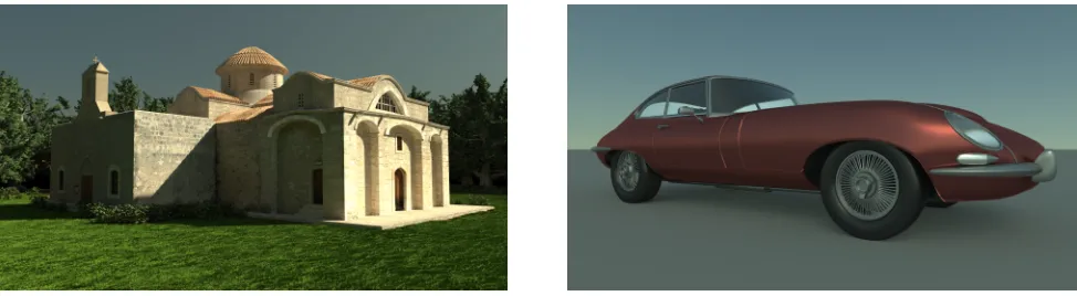
Fig. 2. Rendering of two models (Church and Car) with our neural network sky model trained with the environment maps provided by Kider et al. [1].

II. BACKGROUND ANDRELATEDWORK

This section presents details of existing sky illumination models for both analytic and captured environment maps. This also covers the use of neural networks, in the computer graphics field.

A. Analytic Skylight Models

The CIE (International Commission on Illumination) pro-posed a series of models [7] which aim to approximate sky luminance values. One of the CIE models frequently applied to computed graphics was introduced by Perez et al. [2]. The Perez model is controlled by coefficients A, B, C, D and E each of which is responsible for effects such as in-scattering, out-scattering, and sky clearness. It is described as follows:

Fperez(ξ, γ) = (1 +AeB/cosξ)(1 +CeDγ+Ecos2γ) (1)

where,ξis the zenith angle of the view direction at which the luminance value is evaluated and γ is the angle between sun and view direction.

Nishita and Nakamae [8] proposed a daylight modelling method for clear and overcast skies which calculates light coming from the sun, and scattering due to clouds and water particles in the atmosphere. Nishita et al. [9] modeled the sky by considering the illumination from the sun and sky. Multiple scattering was ignored in this method, instead single scattering by aerosols and air molecules was computed using Rayleigh and Mie scattering. Nishita et al. [10] improved their previous work to handle multiple scattering. They represented the atmosphere as being composed of voxels and used a two-pass method to compute lighting.

A commonly used model was described by Preetham et al. [11], which accounts for both sunlight and skylight. The spectral radiance from the sun was computed taking into account attenuation through the atmosphere. Based on the sky model proposed by Nishita et al. [10], they fitted the parameters for the Perez model. These parameters also depend on turbidity; a term used to approximate the haziness of air. It is the result of light scattering through particles and water vapour in the atmosphere. Low turbidity values generate a very clear sky, and increasing it results in a more hazy sky. Habel et al. [12] represented the Preetham sky model by using spherical harmonics. They fitted the spherical harmonics coefficients to

a function of sun zenith angle and turbidity, and evaluate them at runtime.

Takagi et al. [13] proposed a model consisting of a com-bination of direct sunlight and sky illumination. For sky illumination, they divided the weather conditions into three according to cloud cover and used empirical formulas to find the radiance values. Hoffman and Preetham [14] suggested a straightforward equation for real time implementations de-rived by using constant density for the atmosphere. Bruneton and Neyret [15] also presented a real time method based on precomputing various scattering effects into tables, and performing lookups to reconstruct sky radiance at runtime. In a similar method, Elek and Kmoch [16] dealt with physically based rendering of sky and water bodies. For the rendering of the sky, single and multiple scattering through the atmosphere were simulated. Scattering through the atmosphere was pre-computed and encoded into a lookup table. This lookup table was used to render the sky from an arbitrary observer position and view direction. The full spectral values were also pre-computed to be used in rendering.

Haber et al. [17] proposed a physically based method to render twilight. Their model divides the atmosphere into different layers and uses multiple scattering. The disadvantage of the method is that it can not be rendered in real time.

Hoˇsek and Wilkie [3] presented a model based on an improved version of the Preetham model that can deal with high turbidity values and ground albedo. They calculated light scattering in the atmosphere for a large number of sun positions using an offline path tracing based simulation. The results of the simulation were used to fit the parameters to the modified Preetham model. This model also includes two additional terms. One of them is to deal with the aureole phe-nomenon and other one is to obtain a smooth gradient around the zenith. Their method also provides spectral radiance for a given view and sun direction. Hoˇsek and Wilkie [18] also proposed an improved version of this model which includes attenuated radiance from the solar disk.

this method is based on assumptions about atmospheric con-ditions and the data is only valid at the measurement location. The Radiance [19], [20] rendering package includes two tools for generating a sky model: Gensky and Gendaylit. Gensky produces skies according to the given month, day, time and angular geographical coordinates. It is based on four models, Mardaljevic [21]; the uniform luminance model, the CIE overcast sky model, the CIE clear sky model and the Matsuura intermediate sky model. The Matsuura and Iwata [22] model can represent skies from clear to overcast in a smooth way. To fit the parameters of the sky model based on CIE Standard Clear Sky, they applied regression analysis to a large database. The second tool included in Radiance is Gendaylit which is based on the Perez-All weather model [2]. For more information on clear sky models, see the survey by Sloup [23].

B. Image-Based Lighting

Image-based lighting is a method of lighting virtual environ-ments using captured real world lighting. This has found much use in the film industry, and can produce accurate renderings of objects as if they were placed in the location at which the environment was captured. The method was originally proposed by Blinn and Newell [24]. Debevec [4] further developed and formalised the idea of high dynamic range environment maps. Light entering the full sphere of directions around a point is captured and stored in a map. Typically there exists a mapping from position in the representation of the environment map to a direction on the sphere. This map is then used to render scenes lit by distant lighting as if they were in the position at which the lighting was captured. There are several common representations for environment maps; angular mapping, cube mapping and latitude-longitude mapping, see Banterle et al. [25] for more details. Environment maps can be captured by using a specialised camera hardware such as SpheronVR [5], Panoscan [6] or a light probe which is an image of a specular reflective ball, which captures a reflection of distant lighting. An efficient method for capturing the sun and sky in HDR is described in the work by Stumpfel et al. [26].

C. Artificial Neural Networks

Artificial Neural Networks (ANN), originally proposed by McCulloch and Pitts [27], are a powerful method to find non-linear links between a set of inputs and outputs. They are typically used in the context of supervised machine learning and are often used to implement many tasks such as pattern classification, clustering, optimization etc. More details can be found in the book by Hagan et al. [28]

ANNs have been used a few times recently within the ren-dering. Dachsbacher [29] used ANNs to classify the visibility configurations of objects in virtual scenes. In this method the surface of the object is divided into subsurfaces which are used to obtain the visible fractions of the surface. These fractions are used in co-occurrence matrices to extract feature vectors which are used to train a neural network for visibility analysis.

which use an ANN to approximate the indirect illumination at every scene point in a computationally effective way. Their model is a nonlinear 6D radiance regression function which takes surface position, view direction and lighting direction as input and returns the RGB colour of the indirect illumination. The ANN is trained in an offline pre-pass which calculated the full global illumination at each scene point and direction. This can then be evaluated efficiently at runtime. They clustered scene points and produced separate representations for each cluster. This used multiple smaller networks rather than one extremely large network for the whole scene.

In Meteorological Science, artificial neural networks have been used also to estimate sky luminance. Janjai and Plaon [31] used measured discrete sky luminance data to train a neural network which generates clear, partly cloudy and overcast skies. This only deals with luminance, whereas our model computes colour values. Furthermore, their method used a small number of input directions for training and evaluation, which is not sufficient for image synthesis applications. Work by Zarzalejo et al [32] and Linares-Rodriguez et al. [33] use a neural network to predict solar irradiation on the ground using inputs from satellite data. However, this is not applicable to evaluating sky radiance given a viewing direction.

III. MODELINGSKIES WITHNEURALNETWORKS

The aim of this work is to produce a sky model capable of representing the illumination in existing analytic models and environment maps, with low memory consumption and fast evaluation. Machine learning provides such a generic approach by learning the details of how to predict sky illumination based on minimal inputs. While there are many broad classes of machine learning methods, neural networks provide significant advantages. They are effective at learning continuous functions (Hornik et al. [34]), which makes them applicable to analytic sky models, and have compact storage. In this section a sky illumination model based on neural network is presented.

A. Sky Illumination Model

Sky models attempt to predict the incident radiance due to sun light being scattered in the atmosphere. Typically, models are given an input feature vector Vmodel, which contains a

subset of a full description of the skyV, i.e.Vm⊆V wherem

is a sky model such as Hoˇsek, Preetham or IBL. These models return incident radiance coming from a direction ωview. The

general form of a sky model is:

L(ωview) =Fm(Vm) (2)

whereFmis the sky model andVmis a feature vector which

describes the sky. This feature vector contains information such as sun direction (ωsun), turbidity (t), ground albedo, and

viewing direction (ωview), and any other information required

to describe the process of sky illumination.

For example, in Equation 1, the feature vector for the Perez model is given by Vperez ={ωsun, ωview}, which are

representation, where VIBL = {ωview} is transformed into

θview and φview values used to look up incoming radiance

from the stored environment map.

The aim of this work is to approximate all sky model functions, with a machine learning driven model:

∀ m: FN N(VN N)≈Fm(Vm). (3)

That is, we approximate the sky illuminationFm(Vm)by using

neural networks, FN N(VN N).

B. Neural Network Representation

If we denote the neural network sky representation by Ψ, then the incoming illumination is formulated by using the outputs of the neural network in the following way:

FN N(VN N) =Ls(Ψ(VN N)). (4)

The neural network Ψ encodes the non-linear relationship between the input feature vectorVN N and the RGB triplet in

[0..1).Ls is a scaling function which transforms the outputs

of the neural network to the correct radiance values, which may take values outside the range [0..1).

ANNs are composed of neurons which are separated into several layers known as input, hidden and output layers in a multilayered neural network. These layers are connected by edges which are assigned a weight.

The structure of the ANN is an acyclic graph in which weights are assigned to edges between two neurons in con-secutive layers. Layers have fixed positions where the first and last layers are the input and output layer respectively and the other layers are hidden layers. In order to use an ANN to model sky illumination, various parameters relating to the sky are required as an input and RGB triplets in[0..1)are required as the output. Spectral values could also be approximated using the network, but this work considers standard RGB values. In addition to the neurons in the input and hidden layers the network includes a bias term in these layers, an additional neuron with a constant value of 1. It is connected to the neurons in the following layer. Including a bias term helps to improve training by shifting the outputs of the activation function, which adds nonlinearity to the neural network Ψ.

Ψis a nonlinear mapping from Rq _{to theR}n _whereqand

nare the neuron sizes of the input and output layers.Ψmaps the inputs to the output layer by calculating each intermediate neurons in the following way. Let the weight value between the layer (k) and the previous layer (k−1) bew_jk_kj

(k−1)wherejk=

[1..nk] is the neuron index in the layer(k) with nk neurons.

Then thejk0thoutput (okjk) for thek

0_{thlayer is computed as:}

okjk =f( X

j(k−1)

wjkkj(k−1)∗o

(k−1)

j(k−1)+w

k

jk0), (5)

where the radial basis function, f(x) = ₁₊1_x2, is used as

the activation function. wk_jk0 is the weight assigned to a bias term in the previous layer. Hence the mapping Ψ(VN N) =

{Ψ(VN N)1,Ψ(VN N)2,Ψ(VN N)3} with one hidden layer is

expressed as:

Ψ(VN N)j3=f(

X

j2

w_j3_3j2∗f(X

j1

w_j2_2j1∗(VN N)j1+w

2

j20)

+w_j3

30). (6)

Finally, the outputs of the ANN which consist of RGB values in the range [0..1) are scaled to the correct radiance values, using the scaling function:

Ls(x) = 0.5(

1

x−1). (7)

This function is explained in Section III-C.

1) Input Feature Vector

Fig. 3. Coordinate system used for sun and view directions.

One of the first tasks when designing the neural network Ψ, is to decide on the inputs. As stated in Section III-A, it can be assumed that there exists a feature vectorV containing all information required to fully describe sky illumination. Existing models use a subset of this information as input to their models Vm ⊆ V. Therefore, as the neural network

approximation aims to approximate multiple sky models, the feature vector used as the input which is the combination of the models being approximated. Additionally, a change in the azimuth angle of the sun results in a rotation of the hemisphere. Therefore, we fix the azimuth angle, and only the zenith angleθsun is used in training and evaluation.

If spherical coordinates are used, the outputs of the network are discontinuous between the azimuth angles φ = 2π and φ = 0 which results in a jump in sky illumination values. Therefore, the viewing direction is represented in the Cartesian coordinate system (ωview={vx, vy, vz}), instead of spherical

coordinates as can be seen in the Figure 3. It can also be noted that the relationship between incident radiance and turbidity is highly non-linear. Instead of developing a more complicated neural network to encode this non-linear relationship, we apply a non-linear scaling to the turbidity parameter as an input. It was empirically determined that replacingtwith√tprovided a good approximation to this non-linear relationship.

used the Euclidean distance (d) between the sun and view direction as another input. Another option was to use the dot product of the sun and view directions (cos(γ)). However, this function leads to ambiguities in the input angles γ and π−γleading to worse training results. The Euclidean Distance is equal to the monotonically increasing function 2 sin(0.5γ) which improves the training performance by providing more consistent information related to the position of two directions according to each other. Therefore, the input vector used for the neural network is VN N ={

√

t, θsun, vx, vy, vz, d}.

When we fit to a model which does not use an element of the feature vector VN N, we zero the input, and train as

before. For example, when fitting the neural network to an environment map sequence, the input feature vector contains VN N = {0, θsun, vx, vy, vz, d} as no turbidity calculations

are required. This makes no difference in the evaluation of Equation 6, since the multiplication of the zeroed input with the weights connected to it does not have any effect on the value of the neurons in the hidden and output layers.

2) Structure of the Network

The structure of the ANN requires careful consideration. Using too many neurons can lead to over fitting. On the other hand, if too few neurons are used the network may not be able to train adequately. Using a large number of neurons increases the computational time of evaluation reducing the benefits of using an ANN for computational gains. This section describes the motivation for the choice of the proposed ANN structure.

Fig. 4. Mapping inputs to the RGB colour space with neural network.

The design of the first layer of the neural network has already been discussed above, and consists ofq= 6neurons. The outputs of the neural network are the three RGB colour channels of the sky illumination, therefore the output layer is of size three. An ANN can include multiple hidden layers with combinations of different neuron sizes. However, networks containing multiple hidden layers are slower to evaluate, and more difficult to train, compared using a single hidden layer. Since in our experiments a single hidden layer neural network achieved satisfactory results, the proposed network contains one hidden layer and thus avoids the complexity of training and evaluating multi-layer networks.

Fig. 5. Mapping inputs to the RGB colour space with neural network.

In order to determine the number of neurons in the hidden layer, a series of tests were run on different ANN configu-rations in which the size of the hidden layer was increased sequentially. These tests were performed with Hoˇsek sky model as it has a larger training set, see Section III-C. Each configuration was run 10 times and the average normalized error (based on cross validation method explained in Section IV-A) is shown on the left graph in Figure 5. The graph indicates that the error decreases when the number of neurons are increased. However, this leads to an increase in the time to evaluate the neural network. A metric which takes into account both error and time is efficiency:

(Ψ) = 1

V ar[Ψ]T[Ψ], (8)

whereV aris the variance of the model and T is the time to evaluate the model. It can be concluded from Figure 5 that the neural network structured with a hidden layer of12 neurons is the most efficient model for use in our work. An illustration of the structure of the network can be seen in the Figure 4.

C. Training

The main idea of training the neural network is to minimize the error function, Li et al. [35]:

E(w) =X

j

kFm(Vm)j−FN N(VN N)jk2, j={1,2,3} (9)

wherej represents the RGB colour channel outputs.Fm(Vm)

is the output vector from the model being trained, and is commonly referred to as the target vector. This, combined with the neural network feature vector VN N forms a pair

of vectors called an example ({VN N, Fm(Vm)}j). The set of

examples is known as a training set. The process of finding the optimal weights in the mapping is called training (or learning). The Backpropagation Algorithm is used to train the network via examples. Two basic steps are repeated. Firstly, an input feature vector (VN N) is mapped to the output layer.

The target outputs of the algorithm are the scaled RGB components of the sky illumination as mentioned in Section III-A. These outputs have to be scaled into the range [0..1) through the inverse of the scaling function in Equation 7: L−1

s = 1/(1 + 2x). Since the targets of the network are the

colors of the sky which do not vary significantly according to the view direction, the output values of the network are typically very close to each other. Therefore, the coefficient 2 in the scaling function is used to spread the range of values more evenly over the range [0,1). Using a larger coefficient causes the range of values to again cluster at a small region of the domain.

D. Implementation

The analytical models are trained with turbidity values ranging from 1..10 for the Hoˇsek sky model and from 2..6 for the Preetham sky model. These values are valid for the original methods. 20 sun zenith angles were sampled uniformly between θ = 0 andθ = π/2 at an azimuth angle φ =π are sampled for each turbidity value. View directions are specified by using stratified sampling of the hemisphere. In our implementation, the analytic sky models are trained with10zenith and20azimuth view directions. Increasing the amount of samples does not improve the results drastically, but increases the training time. This sample size was sufficient to train all of the analytic sky models.

For environment map sequences, HDR images are used to train the network. The images are aligned such that the azimuth angle of the sun is aligned for all the input images. Then, for each input environment map, the zenith angle of the sun in each image is calculated automatically by finding the pixel with highest color value. View directions are specified by sampling pixels related to the sky pixels in the image. Valid sky pixels are currently selected by segmenting the sky from any other content, such as trees or buildings. These segmentation processes are currently performed manually, but automatic approaches can be used (similar to [36]). Also pixels tagged as belonging to the sun are not used in training via thresholding.

Since in our method the neural network is trained with a sun azimuth angle of π. A sky model with an arbitrary sun direction{θsun, φsun} is therefore rotated to position the

sun at {θsun, π}. Therefore, the normalized view direction

{vx0, v0y, v0z}is rotated to take this into account:

rotate=φsun−π,

vx=v0x∗cos(rotate) +v 0

y∗sin(rotate),

vy=vy0 ∗cos(rotate)−v 0

x∗sin(rotate),

vz=v0z, (10)

where {vx, vy, vz} forms the correctly rotated input to the

neural network.

This method is amenable to both an efficient CPU and GPU implementation. An advantage to this is that the sky model can be altered without changing any evaluation code. Therefore, differing sky models can be easily swapped with minimal

implementation effort, by simply updating the weights. This is particular useful for GPUs whereby GPU specific imple-mentations of other models are not required and our current implementation, if trained with a sky model on the CPU, will work with little additional changes. Furthermore, evaluation requires only two layers to be computed, and does not involve branching which is ideal for GPU computation.

IV. RESULTS

Sky illumination using ANNs is demonstrated for the analytical models of Preetham et al. [11] and Hoˇsek and Wilkie [3] (henceforth referred to as Preetham and Hoˇsek sky models respectively), and for captured environment maps. When training, the following values were used: learning rate β = 0.01 and momentum µ = 0.9, which is a commonly used momentum value for the backpropagation algorithm, see Li et al. [35]. The learning rate is chosen according to the initial experiments which showed that using a smaller learning rate increases the training time and a larger value decreases the training performance. Therefore a value which balances between these extremes was chosen. These results were obtained on Intel Xeon E5-2620 CPU.

A. RMSE Results

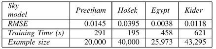
Table 1

Cross validation results for the trained sky models, time in seconds required to train the neural network and the number of examples.

Sky

model Preetham Hoˇsek Egypt Kider

RMSE 0.0145 0.0395 0.0038 0.0118

Training Time (s) 291 195 458 621

Example size 20,000 40,000 25,973 43,295

per image in the validation sets, see Table 1. In our results, the accuracies ranged between 96.05% and 99.62% (as nor-malized RMSE was used) for the chosen validation set. These results can be improved by using more neurons resulting in a higher computational cost. However, the current results are satisfactory and it can be concluded that the sky illumination is learned accurately by the neural network.

We computed irradiance for each sky model and compared it with our ANN representation. The values were computed using the same data sets used for the RMSE results. Irradiance was computed per sun position as:

I=

Z

Ω

L(ωview)cos(θview)dωview, (11)

where Ω is the hemisphere. Table 2 shows the averaged irradiance results obtained and the difference between the original and ANN sky model (unitsW/m2).

Table 2

Cross validation results for irradiance values generated by trained sky models.

Absolute Error Reference Neural Network Difference

Preetham 0.11665 0.11695 0.00030

Hoˇsek 0.03671 0.03838 0.00253

Egypt 0.02472 0.02425 0.00047

Kider 0.10882 0.10419 0.00462

B. Comparative Results

Fig. 6. Examples of the training of ANN with Preetham sky model, for θsun=π∗0.48,t= 4. Left: Reference sky model. Middle: Output of the

ANN. Right: Difference Image.

Fig. 7. Examples of the training of ANN with Hoˇsek sky model, forθsun=

π∗0.3,t= 2. Left: Reference sky model. Middle: Output of the ANN. Right: Difference Image.

We visually validated the results of the training by com-paring a variety of sky scenarios. The outputs of the ANNs trained with Preetham and Hoˇsek sky models exhibited visual similarity to the reference sky models. The difference between the sky models is given with the reference sky and trained sky model is shown in Figure 6 and Figure 7. As can be seen in the difference images, the ANN performs well over the sky; however the neural network representation produces a small amount of low frequency error, especially around the higher frequency regions.

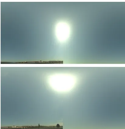
Figure 8 shows the similarity of our ANN representation to a captured environment map. The left half of the image is

Fig. 8. Juxtaposition of the models in one image for different sun positions. Left side: Reference sky model by Kider et al. [1]. Right side: Output of the ANN

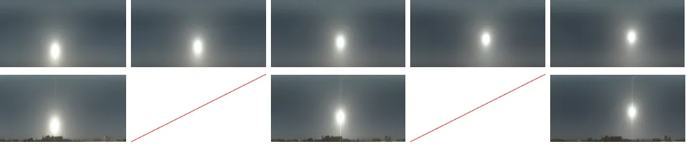
the original environment map, and the right half of the image was computed from the ANN. Figures 1 and 9 demonstrate the ability of the ANN to compute novel sun positions from a captured sequence of environment maps. The top row show skies synthesized with our approach, and bottom shows original captured images. The gaps in the bottom row indicate gaps between captures, which are filled by our method. This enables smooth animations of sky lighting to be generated from discrete environment map captures.

We also rendered two scenes with our method for sky illumi-nation (using path tracing), which are shown in Figure 2. These scenes use the neural network to compute the sky lighting based on the input Kider environment maps. The Church scene additionally includes a directional light to represent the direct sun illumination.

C. Timings

D. Discussion

The neural network based approach presented in this paper currently is trained to produce RGB values. Spectral values could be generated by modifying the output layer to produce spectral values at a number of wavelengths. We generate RGB data in our approach as not all of the methods captured spectral data, for example some of the environment maps used contained only RGB data. Additionally, the feature vector used as an input to our method can be expanded to take into account additional inputs, such as ground albedo used in the Hoˇsek model. This may involve re-computing the size of the hidden layer, however the methodology presented can adapt to these changes.

Our method is an approximation to existing sky models, and environment maps. However, this approximation has a fixed runtime cost, has a small memory footprint, and is generic enough to represent existing models with a high degree of accuracy.

V. CONCLUSION

In this work we have proposed a different approach to the sky illumination problem. We presented a machine learning driven approach to calculate sky illumination for a specific sun position. A single hidden layer neural network was trained to represent analytic sky models and environment maps. The sky illumination returned by the network is accurate when compared with the original sky models. Our approach can be used to extract the sky lighting from captured environ-ment map sequences, and can be used to calculate smooth animation from environment maps captured at discrete times. As our method only requires a small neural network for the representation, it can be efficiently evaluated by both CPU and GPU implementations.

AUTHORS’ BIOGRAPHIES

Pinar Satilmis holds an MSc and a BSc degree in Mathe-matics from Hacettepe University, Turkey. She is currently a PhD candidate at the University of Warwick and a research assistant in Hacettepe University. Her research interests are physically-based rendering and Monte Carlo methods.

email: [email protected]

Thomas Bashford-Rogershas a degree in Computer Science from the University of Bristol and a doctorate in Computer Graphics from the University of Warwick. His research inter-ests include global illumination, raytracing and Monte Carlo methods. He is currently a Research Fellow at the University of Warwick.

email : [email protected]

Alan Chalmers is a Professor of Visualisation at WMG, University of Warwick, UK and a Royal Society Industrial Fellow. He has an MSc with distinction from Rhodes Uni-versity, 1985 and a PhD from University of Bristol, 1991. Chalmers is Founder and Innovation Director of goHDR Ltd. He is Honorary President of Afrigraph, a former Vice President of ACM SIGGRAPH. He has published over 220 papers in journals and international conferences on HDR, high-fidelity virtual environments, multi-sensory perception,

parallel processing and virtual archaeology and successfully supervised 36 PhD students. Chalmers was Chair of EU COST Action IC1005 HDR that co-ordinated HDR research across Europe to facilitate its widespread uptake. He is also a UK representative on IST/37 considering the incorporation of HDR in MPEG.

email: [email protected]

Kurt Debattista is an Associate Professor at the University of Warwick. He has a PhD degree in Computer Science from the University of Bristol, as well as an MSc in Computer Science and an MSc in Psychology. His research interests include physically-based rendering, perceptual imaging, high dynamic range imaging, and parallel computing.

email : [email protected]

REFERENCES

[1] J. T. Kider Jr, D. Knowlton, J. Newlin, Y. K. Li, and D. P. Greenberg, “A framework for the experimental comparison of solar and skydome illumination,”ACM Transactions on Graphics (TOG), vol. 33, no. 6, p. 180, 2014.

[2] R. Perez, R. Seals, and J. Michalsky, “All-weather model for sky luminance distribution-preliminary configuration and validation,”Solar energy, vol. 50, no. 3, pp. 235–245, 1993.

[3] L. Hosek and A. Wilkie, “An analytic model for full spectral sky-dome radiance,”ACM Transactions on Graphics (TOG), vol. 31, no. 4, p. 95, 2012.

[4] P. Debevec, “Rendering synthetic objects into real scenes: Bridging traditional and image-based graphics with global illumination and high dynamic range photography,” inACM SIGGRAPH 2008 classes. ACM, 2008, p. 32.

[5] Spheron, “Last accessed: October, 2014,” http://www.weiss-ag.org/, 2014.

[6] Panoscan, “Last accessed: October, 2014,” http://www.panoscan.com/, 2014.

[7] ISO/CIE. 2004. Technical standard ISO 15469:2004 (CIE S 011/E:2003), “Spatial distribution of daylight-cie standard general sky,”Jointly published by ISO and CIE.

[8] T. Nishita and E. Nakamae, “Continuous tone representation of three-dimensional objects illuminated by sky light,” in ACM SIGGRAPH Computer Graphics, vol. 20, no. 4. ACM, 1986, pp. 125–132. [9] T. Nishita, T. Sirai, K. Tadamura, and E. Nakamae, “Display of the earth

taking into account atmospheric scattering,” inProceedings of the 20th annual conference on Computer graphics and interactive techniques. ACM, 1993, pp. 175–182.

[10] T. Nishita, Y. Dobashi, K. Kaneda, and H. Yamashita, “Display method of the sky color taking into account multiple scattering,” in Pacific Graphics, vol. 96, 1996, pp. 117–132.

[11] A. J. Preetham, P. Shirley, and B. Smits, “A practical analytic model for daylight,” inProceedings of the 26th annual conference on Computer graphics and interactive techniques. ACM Press/Addison-Wesley Publishing Co., 1999, pp. 91–100.

[12] R. Habel, B. Mustata, and M. Wimmer, “Efficient spherical harmonics lighting with the preetham skylight model,”Proceedings of Eurographics Short Papers, 2008.

[13] A. Takagi, H. Takaoka, T. Oshima, and Y. Ogata, “Accurate rendering technique based on colorimetric conception,”ACM SIGGRAPH Com-puter Graphics, vol. 24, no. 4, pp. 263–272, 1990.

[14] N. Hoffman and A. J. Preetham, “Rendering outdoor light scattering in real time,” inProceedings of Game Developer Conference, vol. 2002, 2002, pp. 337–352.

[15] E. Bruneton and F. Neyret, “Precomputed atmospheric scattering,” in Computer Graphics Forum, vol. 27, no. 4. Wiley Online Library, 2008, pp. 1079–1086.

[16] O. Elek and P. Kmoch, “Real-time spectral scattering in large-scale nat-ural participating media,” inProceedings of the 26th Spring Conference on Computer Graphics. ACM, 2010, pp. 77–84.

[17] J. Haber, M. Magnor, and H.-P. Seidel, “Physically-based simulation of twilight phenomena,”ACM Transactions on Graphics (TOG), vol. 24, no. 4, pp. 1353–1373, 2005.

Fig. 9. Skies for consecutive sun positions in a day in Egypt. Top: Results of the ANN trained with environment maps captured in Egypt. Bottom: Corresponding reference images to the ones on the top. The gaps indicate missing reference images which are filled by our model.

[19] G. J. Ward, “The radiance lighting simulation and rendering system,” in Proceedings of the 21st annual conference on Computer graphics and interactive techniques. ACM, 1994, pp. 459–472.

[20] G. W. Larson, R. Shakespeare, C. Ehrlich, J. Mardaljevic, E. Phillips, and P. Apian-Bennewitz,Rendering with radiance: the art and science of lighting visualization. Morgan Kaufmann San Francisco, CA, 1998. [21] J. Mardaljevic, “Daylight simulation: validation, sky models and daylight

coefficients.” 1999.

[22] K. Matsuura and T. Iwata, “A model of daylight source for the daylight illuminance calculations on the all weather conditions,” inProceedings of 3rd International Daylighting Conference, 1990.

[23] J. Sloup, “A survey of the modelling and rendering of the earth’s atmosphere,” inProceedings of the 18th spring conference on Computer graphics. ACM, 2002, pp. 141–150.

[24] J. F. Blinn and M. E. Newell, “Texture and reflection in computer generated images,”Communications of the ACM, vol. 19, no. 10, pp. 542–547, 1976.

[25] F. Banterle, A. Artusi, K. Debattista, and A. Chalmers,Advanced High Dynamic Range Imaging. AK Peters, 2011.

[26] J. Stumpfel, C. Tchou, A. Jones, T. Hawkins, A. Wenger, and P. Debevec, “Direct hdr capture of the sun and sky,” inProceedings of the 3rd inter-national conference on Computer graphics, virtual reality, visualisation and interaction in Africa. ACM, 2004, pp. 145–149.

[27] W. S. McCulloch and W. Pitts, “A logical calculus of the ideas immanent in nervous activity,” The bulletin of mathematical biophysics, vol. 5, no. 4, pp. 115–133, 1943.

[28] M. T. Hagan, H. B. Demuth, M. H. Bealeet al.,Neural network design. Pws Pub. Boston, 1996.

[29] C. Dachsbacher, “Analyzing visibility configurations,”Visualization and Computer Graphics, IEEE Transactions on, vol. 17, no. 4, pp. 475–486, 2011.

[30] P. Ren, J. Wang, M. Gong, S. Lin, X. Tong, and B. Guo, “Global illumination with radiance regression functions,”ACM Transactions on Graphics (TOG), vol. 32, no. 4, p. 130, 2013.

[31] S. Janjai and P. Plaon, “Estimation of sky luminance in the tropics using artificial neural networks: Modeling and performance comparison with the cie model,”Applied Energy, vol. 88, no. 3, pp. 840–847, 2011. [32] L. F. Zarzalejo, L. Ramirez, and J. Polo, “Artificial intelligence

techniques applied to hourly global irradiance estimation from satellite-derived cloud index,” Energy, vol. 30, no. 9, pp. 1685 – 1697, 2005, measurement and Modelling of Solar Radiation and Daylight- Challenges for the 21st Century. [Online]. Available: http://www.sciencedirect.com/science/article/pii/S036054420400249X [33] A. Linares-Rodriguez, J. A. Ruiz-Arias, D. Pozo-Vazquez, and J.

Tovar-Pescador, “An artificial neural network ensemble model for estimating global solar radiation from meteosat satellite images,”Energy, vol. 61, pp. 636–645, 2013.

[34] K. Hornik, M. Stinchcombe, and H. White, “Multilayer feedforward networks are universal approximators,”Neural networks, vol. 2, no. 5, pp. 359–366, 1989.

[35] J. Li, J.-h. Cheng, J.-y. Shi, and F. Huang, “Brief introduction of back propagation (bp) neural network algorithm and its improvement,” in Advances in Computer Science and Information Engineering. Springer, 2012, pp. 553–558.