1 2 3 4 5 6 7 8 9 10 11 12 13 14 15 16 17 18 19 20 21 22 23 24 25 26 27 28 29 30 31 32 33 34 35 36 37 38 39 40 41 42 43 44 45 46 47 48
C
2007 Biometrika Trust
Printed in Great Britain
On the Asymptotic Efficiency of Approximate Bayesian
Computation Estimators
BY WENTAOLI
School of Mathematics, Statistics and Physics, Newcastle University, Newcastle upon Tyne NE1 7RU, U.K.
AND PAULFEARNHEAD
Department of Mathematics and Statistics, Lancaster University, Lancaster LA1 4YF, U.K.
[email protected] SUMMARY
Many statistical applications involve models for which it is difficult to evaluate the likeli-hood, but from which it is relatively easy to sample. Approximate Bayesian computation is a likelihood-free method for implementing Bayesian inference in such cases. We present results on the asymptotic variance of estimators obtained using approximate Bayesian computation in a large-data limit. Our key assumption is that the data is summarized by a fixed-dimensional sum-mary statistic that obeys a central limit theorem. We prove asymptotic normality of the mean of the approximate Bayesian computation posterior. This result also shows that, in terms of asymp-totic variance, we should use a summary statistic that is the same dimension as the parameter vector,p; and that any summary statistic of higher dimension can be reduced, through a linear transformation, to dimensionpin a way that can only reduce the asymptotic variance of the pos-terior mean. We look at how the Monte Carlo error of an importance sampling algorithm that samples from the approximate Bayesian computation posterior affects the accuracy of estima-tors. We give conditions on the importance sampling proposal distribution such that the variance of the estimator will be the same order as that of the maximum likelihood estimator based on the summary statistics used. This suggests an iterative importance sampling algorithm, which we evaluate empirically on a stochastic volatility model.
Some key words: Approximate Bayesian computation; Asymptotics; Dimension Reduction; Importance Sampling; Partial Information; Proposal Distribution.
1. INTRODUCTION
Many statistical applications involve inference about models that are easy to simulate from, but for which it is difficult, or impossible, to calculate likelihoods. In such situations it is possible to use the fact we can simulate from the model to enable us to perform inference. There is a wide class of such likelihood-free methods of inference including indirect inference (Gouri´eroux &
Ronchetti,1993;Heggland & Frigessi,2004), the bootstrap filter (Gordon et al.,1993), simulated
49 50 51 52 53 54 55 56 57 58 59 60 61 62 63 64 65 66 67 68 69 70 71 72 73 74 75 76 77 78 79 80 81 82 83 84 85 86 87 88 89 90 91 92 93 94 95 96
model. Arguably the first approximate Bayesian computation method was that ofPritchard et al.
(1999), and these methods have been popular within population genetics (Beaumont et al.,2002), ecology (Beaumont, 2010) and systems biology (Toni et al.,2009). More recently, there have been applications to areas including stereology (Bortot et al.,2007), finance (Peters et al.,2011) and cosmology (Ishida et al.,2015).
Let K(x) be a density kernel, scaled, without loss of generality, so that maxxK(x) = 1.
Further, let ε >0be a bandwidth. Denote the data by Yobs = (yobs,1, . . . , yobs,n). Assume we
have chosen a finite-dimensional summary statistic sn(Y), and denote sobs =sn(Yobs). If we
model the data as a draw from a parametric density,fn(y|θ), and assume prior,π(θ), then we
define the approximate Bayesian computation posterior as
πABC(θ|sobs, ε)∝π(θ)
ˆ
fn(sobs+εv|θ)K(v)dv, (1)
where fn(s|θ) is the density for the summary statistic implied byfn(y|θ). LetfABC(sobs | θ, ε) =´fn(sobs+εv|θ)K(v)dv. This framework encompasses most implementations of
ap-proximate Bayesian computation. In particular, the use of the uniform kernel corresponds to the popular rejection-based rule (Beaumont et al.,2002).
The idea is that fABC(sobs |θ, ε) is an approximation of the likelihood. The approximate
Bayesian computation posterior, which is proportional to the prior multiplied by this likelihood approximation, is an approximation of the true posterior. The likelihood approximation can be interpreted as a measure of, on average, how close the summary,sn, simulated from the model is
to the summary for the observed data,sobs. The choices of kernel and bandwidth determine the
definition of closeness.
By defining the approximate posterior in this way, we can simulate samples from it using standard Monte Carlo methods. One approach, that we will focus on later, uses importance sam-pling. LetKε(x) =K(x/ε). Given a proposal density,qn(θ), a bandwidth,ε, and a Monte Carlo
sample size, N, an importance sampler would proceed as in Algorithm 1. The set of accepted parameters and their associated weights provides a Monte Carlo approximation toπABC. If we
setqn(θ) =π(θ)then this is just a rejection sampler. In practice sequential importance sampling methods are often used to learn a good proposal distribution (Beaumont et al.,2009).
Algorithm 1. Importance and rejection sampling approximate Bayesian computation 1. Simulateθ1, . . . , θN ∼qn(θ);
2. For eachi= 1, . . . , N, simulateY(i)={y(i) 1 , . . . , y
(i)
n } ∼fn(y|θi);
3. For eachi= 1, . . . , N, acceptθi with probabilityKε{sn(i)−sobs}, wheres (i)
n =sn{Y(i)};
and define the associated weight aswi =π(θi)/qn(θi).
There are three choices in implementing approximate Bayesian computation: the choice of summary statistic, the choice of bandwidth, and the Monte Carlo algorithm. For importance sampling, the last of these involves specifying the Monte Carlo sample size,N, and the proposal density,qn(θ). These, roughly, relate to three sources of approximation. To see this, note that as
ε→0we would expect (1) to converge to the posterior givensobs(Fearnhead & Prangle,2012).
Thus the choice of summary statistic governs the approximation, or loss of information, between using the full posterior distribution and using the posterior given the summary. The value ε
97 98 99 100 101 102 103 104 105 106 107 108 109 110 111 112 113 114 115 116 117 118 119 120 121 122 123 124 125 126 127 128 129 130 131 132 133 134 135 136 137 138 139 140 141 142 143 144
which together affect, say, the probability of acceptance in step 3 of Algorithm 1. Having a higher-dimensional summary statistic, or a smaller value ofε, will tend to reduce this acceptance probability and hence increase the Monte Carlo error.
This work aims to study the interaction between the three sources of error, in the case where the summary statistics obey a central limit theorem for largen. We are interested in the efficiency of approximate Baysian computation, where by efficiency we mean that an estimator obtained from running Algorithm 1 has the same rate of convergence as the maximum likelihood estimator for the parameter given the summary statistic. In particular, this work is motivated by the question of whether approximate Bayesian computation can be efficient asn→ ∞ if we have a fixed Monte Carlo sample size. Intuitively this appears unlikely. For efficiency we will needε→0as
n→ ∞, and this corresponds to an increasingly strict condition for acceptance. Thus we may imagine that the acceptance probability will necessarily tend to zero asnincreases, and thus we will need an increasing Monte Carlo sample size to compensate for this.
However our results show that Algorithm1can be efficient if we choose an appropriate pro-posal distribution. The propro-posal distribution needs to have a suitable scale and location and have appropriately heavy tails. If we use an appropriate proposal distribution and have a summary statistic of the same dimension as the parameter vector then the posterior mean of approximate Bayesian computation is asymptotically unbiased with a variance that is1 +O(1/N)times that of the estimator maximising the likelihood of the summary statistic. This is similar to asymptotic results for indirect inference (Gouri´eroux & Ronchetti,1993;Heggland & Frigessi,2004). Our results also lend theoretical support to methods that choose the bandwidth indirectly by speci-fying the proportion of samples that are accepted, as this leads to a bandwidth which is of the optimal order inn.
We first prove a Bernstein-von Mises type theorem for the posterior mean of approximate Bayesian computation. This is a non-standard convergence result, as it is based on the partial information contained in the summary statistics. For related convergence results seeClarke &
Ghosh(1995) and Yuan & Clarke(2004), though these do not consider the case when the
di-mension of the summary statistic is larger than that of the parameter. Dealing with this case introduces extra challenges.
Our convergence result for the posterior mean of approximate Bayesian computation has prac-tically important consequences. It shows that any d-dimensional summary with d > p can be projected to ap-dimensional summary statistic without any loss of information. Furthermore it shows that using a summary statistic of dimensiond > pcan lead to an increased bias, so the asymptotic variance can be reduced if the optimalp-dimensional projected summary is used in-stead. If ad-dimensional summary is used, withd > p, it suggests choosing the variance of the kernel to match the variance of the summary statistics.
This paper adds to a growing literature on the theoretical properties of approximate Bayesian computation. Initial results focussed on comparing the bias of approximate Bayesian computa-tion to the Monte Carlo error, and how these depend on the choice ofε. The convergence rate of the bias is shown to beO(ε2)in various settings (e.g.Barber et al.,2015). This can then be used to consider how the choice ofεshould depend on the Monte Carlo sample size so as to balance bias and Monte Carlo variability (Blum,2010;Barber et al.,2015;Biau et al.,2015). There has also been work on consistency of approximate Bayesian computation estimators.Marin et al.
145 146 147 148 149 150 151 152 153 154 155 156 157 158 159 160 161 162 163 164 165 166 167 168 169 170 171 172 173 174 175 176 177 178 179 180 181 182 183 184 185 186 187 188 189 190 191 192
shows that for many implementations of approximate Bayesian computation, the posterior will over-estimate the uncertainty in the parameter estimate that it gives.
Finally, a number of papers have looked at the choice of summary statistics (e.g.Wegmann
et al.,2009;Blum,2010;Prangle et al.,2014). Our Theorem1gives insight into this. As
men-tioned above, this result shows that, in terms of minimising the asymptotic variance, we should use a summary statistic that is of the same dimension as the number of parameters. In particular it supports the suggestion inFearnhead & Prangle(2012) of having one summary per parameter, with that summary approximating the maximum likelihood estimator for that parameter.
2. NOTATION ANDSET-UP
Denote the data byYobs = (yobs,1, . . . , yobs,n), where nis the sample size, and each
obser-vation,yobs,i, can be of arbitrary dimension. We make no assumption directly on the data, but
make assumptions on the distribution of the summary statistics. We consider the asymptotics as
n→ ∞, and denote the density ofYobs byfn(y|θ), whereθ∈P⊂Rp. We letθ0 denote the
true parameter value, andπ(θ)its prior distribution. For a setA, letAcbe its complement with
respect to the whole space.
We assume thatθ0 is in the interior of the parameter space, and that the prior is differentiable
in a neighbourhood of the true parameter:
CONDITION1. There exists some δ0 >0, such that P0={θ:|θ−θ0|< δ0} ⊂P, π(θ)∈ C1(P0)andπ(θ0)>0.
To implement approximate Bayesian computation we will use a d-dimensional summary statistic, sn(Y)∈Rd; for example a vector of sample means of appropriately chosen
func-tions. We assume thatsn(Y)has a density function, which depends onn, and we denote this by
fn(s|θ). We will use the shorthandSnto denote the random variable with densityfn(s|θ). In
approximate Bayesian computation we use a kernel,K(x), with maxxK(x) = 1, and a
band-width ε >0. As we vary n we will often wish to vary ε, and in these situations denote the bandwidth byεn. For Algorithm1we require a proposal distribution,qn(θ), and allow for this to depend on n. We assume the following conditions on the kernel, which are satisfied by all commonly used kernels,
CONDITION2. The kernel satisfies (i) ´ vK(v)dv= 0; (ii) ´ Ql
k=1vikK(v)dv <∞ for any coordinates(vi1, . . . , vil)ofv andl≤p+ 6; (iii)K(v)∝K(kvk
2
Λ)wherekvk2Λ=vTΛv and Λ is a positive-definite matrix, and K(v) is a decreasing function of kvkΛ; (iv)K(v) = O(e−c1kvkαΛ1)for someα
1 >0andc1 >0askvkΛ→ ∞.
For a real functiong(x)denote itskth partial derivative atx=x0 byDxkg(x0), the gradient
function by Dxg(x0) and the Hessian matrix byHxg(x0). To simplify the notations,Dθk,Dθ
andHθ are written asDk, DandH respectively. For a series xnwe use the notation that for
large enoughn,xn= Θ(an)if there exists constantsm andM such that0< m <|xn/an|< M <∞, andxn= Ω(an)if|xn/an| → ∞. For two square matricesAandB, we sayA≤Bif
B−Ais semi-positive definite, andA < BifB−Ais positive definite.
Our theory will focus on estimates of some function,h(θ), ofθ, which satisfies differentiability and moment conditions that will control the remainder terms in a Taylor-expansions.
CONDITION3. The kth coordinate of h(θ), hk(θ), satisfies (i) hk(θ)∈C1(P0); (ii) Dkh(θ0)6= 0; and (iii)
´
hk(θ)2π(θ)dθ <∞.
193 194 195 196 197 198 199 200 201 202 203 204 205 206 207 208 209 210 211 212 213 214 215 216 217 218 219 220 221 222 223 224 225 226 227 228 229 230 231 232 233 234 235 236 237 238 239 240
CONDITION4. There exists a sequencean, withan→ ∞asn→ ∞, ad-dimensional vector s(θ)and ad×dmatrixA(θ), such that for allθ∈P0,
an{Sn−s(θ)} →N{0, A(θ)}, n→ ∞,
with convergence in distribution. We also assume thatsobs→s(θ0)in probability. Furthermore, (i) s(θ)∈C1(P0) andA(θ)∈C1(P0), and A(θ) is positive definite for θ∈P0; (ii) for any δ >0there exists aδ0 >0such thatks(θ)−s(θ0)k> δ0for allθsatisfyingkθ−θ0k> δ; (iii) I(θ) =Ds(θ)TA−1(θ)Ds(θ)has full rank atθ=θ
0.
Under Condition4,anis the rate of convergence in the central limit theorem. If the data are independent and identically distributed, and the summaries are sample means of functions of the data or of quantiles, then an=n1/2. In most applications the data will be dependent, but if summaries are sample means (Wood,2010), quantiles (Peters et al.,2011;Allingham et al.,
2009;Blum & Franc¸ois,2010) or linear combinations thereof (Fearnhead & Prangle,2012) then
a central limit theorem will often still hold, thoughanmay increase more slowly thann1/2. Part (ii) of Condition 4 is required for the true parameter to be identifiable given only the summary of data. The asymptotic variance of the summary-based maximum likelihood estimator forθisI−1(θ0)/a2n. Condition (iii) ensures that this variance is valid at the true parameter.
We next require a condition that controls the difference between fn(s|θ) and its limit-ing distribution for θ∈P0. Let N(x;µ,Σ) be the normal density at x with mean µ and variance Σ. Define fne(s|θ) =N{s;s(θ), A(θ)/a2n} and the standardized random variable
Wn(s) =anA(θ)−1/2{s−s(θ)}. LetfeWn(w|θ)andfWn(w|θ)be the density ofWn(s)when
s∼fen(s|θ) andfn(s|θ) respectively. The condition below requires that the difference be-tween fWn(w|θ) and its Edgeworth expansion feWn(w|θ) is o(a
−2/5
n ) and can be bounded
by a density with exponentially decreasing tails. This is weaker than the standard requirement,
o(a−n1), for the remainder in the Edgeworth expansion.
CONDITION5. There exists αn satisfyingαn/an2/5→ ∞ and a densityrmax(w) satisfying Condition2(ii)-(iii) whereK(v)is replaced withrmax(w), such thatsupθ∈P0αn|fWn(w|θ)−
e
fWn(w|θ)| ≤c3rmax(w)for some positive constantc3.
The following condition further assumes thatfn(s|θ)has exponentially decreasing tails with
rate uniform in the support ofπ(θ).
CONDITION6. The following statements hold: (i)rmax(w)satisfies Condition2(iv); and (ii) supθ∈Pc
0fWn(w|θ) =O(e
−c2kwkα2)askwk → ∞for some positive constantsc
2andα2, and A(θ)is bounded inP.
3. POSTERIOR MEAN ASYMPTOTICS
We first ignore any Monte Carlo error, and focus on the ideal estimator from approximate Bayesian computation. This is the posterior mean,hABC, where
hABC=EπABC{h(θ)|sobs}=
ˆ
h(θ)πABC(θ|sobs, εn).
241 242 243 244 245 246 247 248 249 250 251 252 253 254 255 256 257 258 259 260 261 262 263 264 265 266 267 268 269 270 271 272 273 274 275 276 277 278 279 280 281 282 283 284 285 286 287 288
To understand the effect of these two sources of error, we derive results for the asymptotic dis-tributions ofhABCand the likelihood-based estimators, including the summary-based maximum
likelihood estimator and the summary-based posterior mean, where we consider randomness solely due to the randomness of the data. LetTobs =anA(θ0)−1/2{sobs−s(θ0)}.
THEOREM1. Assume Conditions1–6.
(i) LetˆθMLES =argmaxθ∈Plogfn(sobs|θ). Forhs =h(ˆθMLES)orE{h(θ)|sobs},
an{hs−h(θ0)} →N{0, Dh(θ0)TI−1(θ0)Dh(θ0)}, n→ ∞,
with convergence in distribution.
(ii) Definec∞= limn→∞anεn. Let Z be the weak limit of Tobs, which has a standard normal distribution, andR(c∞, Z)be a random vector with mean zero that is defined in the Supple-mentary Material. Ifεn=o(a
−3/5 n ), then
an{hABC−h(θ0)} →Dh(θ0)T{I(θ0)−1/2Z+R(c∞, Z)}, n→ ∞,
with convergence in distribution. If either (i)εn=o(a−n1); (ii)d=p; or (iii) the covariance matrix of K(v)is proportional toA(θ0); thenR(c∞, Z) = 0. For other cases, the variance ofI(θ0)−1/2Z+R(c∞, Z)is no less thanI−1(θ0).
Theorem1(i) shows the validity of posterior inference based on the summary statistics. Re-gardless of the sufficiency and dimension of sobs, the posterior mean based on the summary
statistics is consistent and asymptotically normal with the same variance as the summary-based maximum likelihood estimator.
Denote the bias of approximate Bayesian computation,hABC−E{h(θ)|sobs}, by biasABC.
The choice of bandwidth impacts the size of the bias. Theorem1 (ii) indicate two regimes for the bandwidth for which the posterior mean of approximate Bayesian computation has good properties.
The first case is when εn is o(1/an). For this regime the posterior mean of approximate Bayesian computation always has the same asymptotic distribution as that of the true poste-rior given the summaries. The other case is whenεn iso(an−3/5)but noto(n−1). We obtain the
same asymptotic distribution if eitherd=por we choose the kernel variance to be proportional to the variance of the summary statistics. In general for this regime of εn,hABC will be less
efficient than the summary-based maximum likelihood estimator.
Whend > p, Theorem1(ii) shows that biasABCis non-negligible and can increase the
asymp-totic variance. This is because the leading term of biasABC is proportional to the average of v=s−sobs, the difference between the simulated and observed summary statistics. Ifd > p,
the marginal density of v is generally asymmetric, and thus is no longer guaranteed to have a mean of zero. One way to ensure that there is no increase in the asymptotic variance is to choose the variance of the kernel to be proportional to the variance of the summary statistics.
The loss of efficiency we observe in Theorem1(ii) ford > pgives an advantage for choosing a summary statistic withd=p. The following proposition shows that for any summary statistic of dimension d > p we can find a new p-dimensional summary statistic without any loss of information. The proof of the proposition is trivial and hence omitted.
289 290 291 292 293 294 295 296 297 298 299 300 301 302 303 304 305 306 307 308 309 310 311 312 313 314 315 316 317 318 319 320 321 322 323 324 325 326 327 328 329 330 331 332 333 334 335 336
Theorem1leads to following natural definition.
DEFINITION 1. Assume that the conditions of Theorem1hold. Then theasymptotic variance
ofhABCis
AVhABC =
1 a2
n
Dh(θ0)TIABC−1 (θ0)Dh(θ0).
4. ASYMPTOTIC PROPERTIES OFREJECTION ANDIMPORTANCESAMPLINGALGORITHM
4·1. Asymptotic Monte Carlo Error
We now consider the Monte Carlo error involved in estimatinghABC. Here we fix the data and
consider solely the stochasticity of the Monte Carlo algorithm. We focus Algorithm1. Remember thatN is the Monte Carlo sample size. Fori= 1, . . . , N,θiis the proposed parameter value and
wiis its importance sampling weight. Letφibe the indicator that is 1 if and only ifθiis accepted
in step 3 of Algorithm1and letNacc=PNi=1φibe the number of accepted parameter.
ProvidedNacc≥1we can estimatehABCfrom the output of Algorithm1with
b
h= N
X
i=1
h(θi)wiφi
.XN
i=1 wiφi.
Define the acceptance probability:
pacc,q = ˆ
q(θ)
ˆ
fn(s|θ)Kε(s−sobs)dsdθ,
and the density of the accepted parameter:
qABC(θ|sobs, ε) =
qn(θ)fABC(sobs|θ, ε)
´
qn(θ)fABC(sobs |θ, ε)dθ .
Finally, define
ΣIS,n =EπABC
(h(θ)−hABC)2
πABC(θ|sobs, εn) qABC(θ|sobs, εn)
,
ΣABC,n =p−acc1,qnΣIS,n, (2)
whereΣIS,n is the importance sampling variance withπABC as the target density andqABC as
the proposal density. Note thatpacc,qn andΣIS,n, and henceΣABC,n, depend onsobs.
Standard results give the following asymptotic distribution ofbh.
PROPOSITION2. For a givennandsobs, ifhABCandΣABC,nare finite, then N1/2(bh−hABC)→N(0,ΣABC,n),
in distribution asN → ∞.
This proposition motivates the following definition.
DEFINITION 2. For a given nand sobs, assume that the conditions of Proposition 2 hold. Then the asymptotic Monte Carlo variance ofbhis
MCV b
h = 1
337 338 339 340 341 342 343 344 345 346 347 348 349 350 351 352 353 354 355 356 357 358 359 360 361 362 363 364 365 366 367 368 369 370 371 372 373 374 375 376 377 378 379 380 381 382 383 384
4·2. Asymptotic efficiency
We have defined the asymptotic variance asn→ ∞ofhABC, and the asymptotic Monte Carlo
variance, asN → ∞ofbh. The error ofhABCwhen estimatingh(θ0)and the Monte Carlo error ofbhwhen estimatinghABCare independent, which suggests the following definition.
DEFINITION3. Assume the conditions of Theorem1, and thathABCandΣABC,nare bounded in probability for anyn. Then theasymptotic varianceofbhis
AV bh
= 1
a2 n
h(θ0)TIABC−1 (θ0)Dh(θ0) + 1
NΣABC,n.
We can interpret the asymptotic variance ofhbas a first-order approximation to the variance of our Monte Carlo estimator for both largenandN. We wish to investigate the properties of this asymptotic variance, for large but fixedN, asn→ ∞. The asymptotic variance itself depends on
n, and we would hope it would tend to zero asnincreases. Thus we will study the ratio of AV bh
to AVMLES, where, by Theorem1, the latter isa−2
n h(θ0)TI−1(θ0)Dh(θ0). This ratio measures the
efficiency of our Monte Carlo estimator relative to the maximum likelihood estimator based on the summaries; it quantifies the loss of efficiency from using a non-zero bandwidth and a finite Monte Carlo sample size.
We will consider how this ratio depends on the choice ofεnandqn(θ). Thus we introduce the
following definition:
DEFINITION4. For a choice ofεnandqn(θ), we define the asymptotic efficiency ofbhas AE
b
h = limn→∞
AVMLES AV
b
h .
If this limiting value is zero, we say thatbhis asymptotically inefficient.
We will investigate the asymptotic efficiency ofbh under the assumption of Theorem 1that
εn=o(a
−3/5
n ). We shall see that the convergence rate of the importance sampling varianceΣIS,n
depends on how largeεnis relative toan, and so we further definean,ε=aniflimn→∞anεn<
∞andan,ε =ε−n1 otherwise.
If our proposal distribution in Algorithm1is either the prior or the posterior, then the estimator is asymptotically inefficient:
THEOREM2. Assume the conditions of Theorem1. (i) Ifqn(θ) =π(θ),pacc,qn = Θp(ε
d na
d−p
n,ε )andΣIS,n = Θp(a−n,ε2). (ii) Ifqn(θ) =πABC(θ|sobs, εn),pacc,qn= Θp(ε
d
nadn,ε)andΣIS,n = Θp(apn,ε).
In both casesbhis asymptotically inefficient.
The result in part (ii) shows a difference from standard importance sampling settings, where using the target distribution as the proposal leads to an estimator with no Monte Carlo error.
The estimatorbhis asymptotically inefficient because the Monte Carlo variance decays more slowly than1/a2nasn→ ∞. However this is caused by different factors in each case.
To see this, consider the acceptance probability of a value ofθand corresponding summary
snsimulated in one iteration of Algorithm1. This acceptance probability depends on sn−sobs
εn =
1
385 386 387 388 389 390 391 392 393 394 395 396 397 398 399 400 401 402 403 404 405 406 407 408 409 410 411 412 413 414 415 416 417 418 419 420 421 422 423 424 425 426 427 428 429 430 431 432
wheres(θ), defined in Condition4, is the limiting value ofsnasn→ ∞if data is sampled from the model for parameter valueθ. By Condition4, the first and third bracketed terms within the square brackets on the right-hand side are Op(a−n1). If we sampleθfrom the prior the middle term isOp(1), and thus (3) will blow up as εn goes to zero. Hence pacc,π goes to zero as εn
goes to zero, which causes the estimate to be inefficient. If we sample from the posterior, then by Theorem1we expect the middle term to also beOp(a−n1). Hence (3) is well behaved asn→ ∞, andpacc,π is bounded away from zero, provided eitherεn= Θ(an−1)orεn= Ω(a−n1).
However, if we use πABC(θ|sobs, εn) as a proposal distribution, the estimates are still
in-efficient due to an increasing variance of the importance weights: as nincreases the proposal distribution is more and more concentrated aroundθ0, whileπdoes not change.
4·3. Efficient Proposal Distributions
Consider proposing the parameter value from a location-scale family. That is our proposal is of the formσnΣ1/2X+µn, whereX ∼q(·),E(X) = 0and var(X) =Ip. This defines a general form of proposal density, where the center,µn, the scale rate,σn, the scale matrix,Σ and the
base density,q(·), all need to be specified. We will give conditions under which such a proposal density results in estimators that are efficient.
Our results are based on an expansion of πABC(θ|sobs, εn). Consider the rescaled
ran-dom variablest=an,ε(θ−θ0)andv=ε−n1(s−sobs). Recall thatTobs=anA(θ0)−1/2{sobs− s(θ0)}. Define an unnormalised joint density oftandvas
gn(t, v;τ) =
Nh{Ds(θ0) +τ}t;anεnv+A(θ0)1/2Tobs, A(θ0)
i
K(v), anεn→c <∞,
Nh{Ds(θ0) +τ}t;v+an1εnA(θ0)1/2Tobs,a21
nε2nA(θ0)
i
K(v), anεn→ ∞,
and further definegn(t;τ) = ´
gn(t, v;τ)dv. For large n, and for the rescaled variable t, the
leading term of πABC is then proportional to gn(t; 0). For both limits of anεn, gn(t;τ) is a
continuous mixture of normal densities with the kernel density determining the mixture weights. Our main theorem requires conditions on the proposal density. First, thatσn=a−n,ε1 andcµ= σn−1(µn−θ0)isOp(1). This ensures that under the scaling oft, asn→ ∞, the proposal is not
increasingly over-dispersed compared to the target density, and the acceptance probability can be bounded away from zero. Second, that the proposal distribution is sufficiently heavy-tailed:
CONDITION7. There exist positive constantsm1andm2satisfyingm12Ip < Ds(θ0)TDs(θ0) andm2Id< A(θ0),α∈(0,1),γ ∈(0,1)andc∈(0,∞), such that for anyλ >0,
sup t∈Rp
N(t; 0, m−12m−22γ−1)
q{Σ−1/2(t−c)} <∞, sup t∈Rp
Kα(kλtk2)
q{Σ−1/2(t−c)} <∞, sup t∈Rp
rmax(km1m2γ1/2tk2) q{Σ−1/2(t−c)} <∞,
wherermax(·)satisfiesrmax(v) =rmax(kvk2Λ), and for any random series cn inRp satisfying cn=Op(1),
sup t∈Rp
q(t) q(t+cn)
=Op(1).
433 434 435 436 437 438 439 440 441 442 443 444 445 446 447 448 449 450 451 452 453 454 455 456 457 458 459 460 461 462 463 464 465 466 467 468 469 470 471 472 473 474 475 476 477 478 479 480
THEOREM3. Assume the conditions of Theorem1. If the proposal densityqn(θ)is
βπ(θ) + (1−β) 1
σnp|Σ|1/2
q{σn−1Σ−1/2(θ−µn)},
where β ∈(0,1), q(·) and Σ satisfy Condition 7, σn=a−n,ε1 and cµ is Op(1), then pacc,qn = Θp(εdnan,εd )andΣIS,n=Op(a−n,ε2). Then ifεn= Θ(a−n1),AE
b
h = Θp(1). Furthermore, ifd=p,AE
b
h = 1−K/(N +K)for some constantK.
The mixture withπ(θ) here is to control the importance weight in the tail area (Hesterberg,
1995). It is not clear whether this is needed in practice, or is just a consequence of the approach taken in the proof.
Theorem 3 shows that with a good proposal distribution, if the acceptance probability is bounded away from zero asnincreases, the threshold εn will have the preferred rateΘ(a−n1).
This supports using the acceptance rate to choose the threshold based on aiming for an appropri-ate proportion of acceptances (Del Moral et al.,2012;Biau et al.,2015).
In practice,σn andµn need to be adaptive to the observations since they depend onn. For q(·)andΣ, the following proposition gives a practical suggestion that satisfies Condition7. Let
T(·;γ)be the multivariatetdensity with degree of freedomγ. The following result says that it is theoretically valid to choose anyΣif atdistribution is chosen as the base density.
PROPOSITION3. Condition7is satisfied forq(θ) =T(θ;γ)with anyγ >0and anyΣ. Proof. The first part of Condition 7 follows as thet-density is heavy tailed relative to the normal density,K(·)andrmax(·). The second part can be verified easily.
4·4. Iterative Importance Sampling
Taken together, Theorem3and Proposition3suggest proposing from the mixture ofπ(θ)and atdistribution with the scale matrix and center approximating those ofπABC(θ). We suggest the
following iterative procedure, similar in spirit to that ofBeaumont et al.(2009). Algorithm 2. Iterative importance sampling approximate Bayesian computation
Input a mixture weightβ, a sequence of acceptance rates{pk}, and a location-scale family. Setq1(θ) =π(θ).
Fork= 1, . . . , K:
1. Run Algorithm 1 with simulation sizeN0, proposal densityβπ(θ) + (1−β)qk(θ)and
acceptance ratepk, and record the bandwidthεk.
2. Ifεk−1−εkis smaller than some positive threshold, stop. Otherwise, letµk+1andΣk+1
be the empirical mean and variance matrix of the weighted sample from step 1, and let
qk+1(θ)be the density with centreµk+1and variance matrix2Σk+1.
3. Ifqk(θ)is close toqk+1(θ)orK=Kmax, stop. Otherwise, return to step1.
After the iteration stops at theKthstep, run Algorithm 1 with the proposal densityβπ(θ) + (1−
β)qK+1(θ),N−KN0simulations andpK+1.
In this algorithm,N is the number of simulations allowed by the computing budget,N0 < N
and{pk}is a sequence of acceptance rates, which we use to choose the bandwidth. The maxi-mum valueKmaxofKis set such thatKmaxN0=N/2. The rule for choosing the new proposal
distribution is based on approximating the mean and variance of the density proportional to
π(θ)fABC(sobs|θ, ε)1/2, which is optimal (Fearnhead & Prangle,2012). It can be shown that
re-481 482 483 484 485 486 487 488 489 490 491 492 493 494 495 496 497 498 499 500 501 502 503 504 505 506 507 508 509 510 511 512 513 514 515 516 517 518 519 520 521 522 523 524 525 526 527 528
spectively. For the mixture weight,β, we suggest a small value, and use0.05in the simulation study below.
5. NUMERICALEXAMPLES
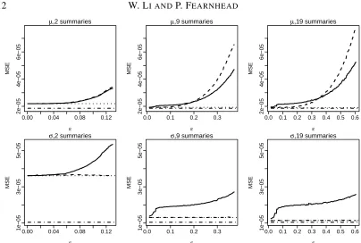
5·1. Gaussian Likelihood with Sample Quantiles
This examples illustrates the results in Section 3 with an analytically tractable problem. As-sume the observations Yobs = (y1, . . . , yn) follow the univariate normal distribution N(µ, σ)
with true parameter values(1,21/2). Consider estimating the unknown parameter (µ, σ) with the uniform prior in the region[−10,10]×[0,10]using Algorithm 1. The summary statistic is
(ebqα1/2, . . . , ebqαd/2)where b
qαis the sample quantile ofYobsfor probabilityα.
The results for data sizen= 105 are presented. Smaller sizes from102 to104 show similar patterns. The probabilitiesα1, . . . , αdfor calculating quantiles are selected with equal intervals
in (0,1), and d= 2,9 and19 were tested. In order to investigate the Monte Carlo error-free performance,N is chosen to be large enough that the Monte Carlo errors were negligible. We compare the performances ofθABC, the maximum likelihood estimator based on the summary
statistics and the maximum likelihood estimator based on the full dataset. Since the dimension reduction matrixCin Proposition1can be obtained analytically, the performance ofθABCusing
the originald-dimension summary is compared with that using the2-dimension summary. The results of mean square error are presented in Figure1.
The phenomena implied by Theorem1and Proposition1can be seen in this example, together with the limitations of these results. First,E{h(θ)|sobs}, equivalent toθABCwith small enough ε, and the maximum likelihood estimator based on the same summaries, have similar accuracy. Second, when εis small, the mean square error ofθABC is the same as that of the maximum
likelihood based on the summary. When ε becomes larger, for d >2 the mean square error increases more quickly than for d= 2. This corresponds to the impact of the additional bias whend > p.
For all cases, the two-dimensional summary obtained by projecting the originaldsummaries is, for smallε, as accurate as the maximum likelihood estimator given the originaldsummaries. This indicates that the lower-dimensional summary contains the same information as the original one. For largerε, the performance of the reduced-dimension summaries is not stable, and is in fact worse than the original summaries for estimatingµ. This deterioration is caused by the bias ofθABC, which for largerε, is dominated by higher order terms inεwhich could be ignored in
our asymptotic results.
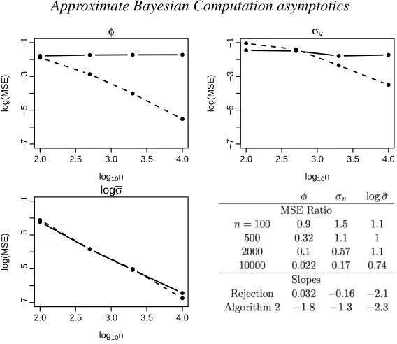
5·2. Stochastic Volatility with AR(1) Dynamics
We consider a stochastic volatility model from Sandmann & Koopman (1998) for the de-meaned returns of a portfolio. Denote this return for thetth time-period asyt. Then
xt=φxt−1+ηt, ηt∼N(0, σ2η); yt=σext/2ξn, ξt∼N(0,1),
whereηtandξtare independent, andxtis a latent state that quantifies the level of volatility for
time-period t. By the transformationyt∗= logyt2 andξt∗= logξ2t, the observation equation in the state-space model can be transformed to
yn∗ = 2 logσ+xn+ξn∗, exp(ξ∗n)∼χ21, (4)
which is linear and non-Gaussian.
529 530 531 532 533 534 535 536 537 538 539 540 541 542 543 544 545 546 547 548 549 550 551 552 553 554 555 556 557 558 559 560 561 562 563 564 565 566 567 568 569 570 571 572 573 574 575 576
0.00 0.04 0.08 0.12
2e−05
4e−05
6e−05
µ,2 summaries
ε
MSE
0.0 0.1 0.2 0.3
2e−05
4e−05
6e−05
µ,9 summaries
ε
MSE
0.0 0.1 0.2 0.3 0.4 0.5 0.6
2e−05
4e−05
6e−05
µ,19 summaries
ε
MSE
0.00 0.04 0.08 0.12
1e−05
3e−05
5e−05
σ,2 summaries
ε
MSE
0.0 0.1 0.2 0.3
1e−05
3e−05
5e−05
σ,9 summaries
ε
MSE
0.0 0.1 0.2 0.3 0.4 0.5 0.6
1e−05
3e−05
5e−05
σ,19 summaries
ε
[image:12.612.82.486.76.348.2]MSE
Fig. 1: Illustration of results in Section 3. Mean square errors of point estimates for200data sets are reported. Point estimates compared includeθABCusing the original summary statistic (solid) and the transformed summary statistic
(dashed), the dimension of which is reduced to2according to Proposition1, the maximum likelihood estimates based on the original summary statistic (dotted) and the full data set (dash-dotted).
importance proposal for largenby comparing with rejection sampling. In the iterative algorithm, atdistribution with 5 degrees of freedom is used to constructqk.
Consider estimating the parameter(φ, ση,logσ)under a uniform prior in the region[0,1)×
[0.1,3]×[−10,−1]. The setting with the true parameter (φ, ση,logσ) = (0.9,0.675,−4.1)is
studied. We use a 3-dimensional summary statistic that stores the mean, variance and lag-1 au-tocovariance of the transformed data. If there were no noise in the state equation forξn∗, then this would be a sufficient statistic ofY∗, and hence is a natural choice for the summary statistic. The uniform kernel is used in the accept-reject step.
We evaluate rejection sampling and iterative importance sampling methods on data of length
n= 100,500,2000and10000; and useN = 40000Monte Carlo simulations. For iterative im-portance sampling, the sequence {pk}has the first five values decreasing linearly from 5%to 1%, and later values being 1%. We further setN0 = 2000, and Kmax= 10. For the rejection
sampler acceptance probabilities of both 5%and1%were tried and5%was chosen as it gave better performance. The simulation results are shown in Figure2.
577 578 579 580 581 582 583 584 585 586 587 588 589 590 591 592 593 594 595 596 597 598 599 600 601 602 603 604 605 606 607 608 609 610 611 612 613 614 615 616 617 618 619 620 621 622 623 624
● ● ● ●
2.0 2.5 3.0 3.5 4.0
−7
−5
−3
−1
φ
log10n
log(MSE)
●
●
●
●
● ●
● ●
2.0 2.5 3.0 3.5 4.0
−7
−5
−3
−1
σv
log10n
log(MSE)
●
●
●
●
●
●
●
●
2.0 2.5 3.0 3.5 4.0
−7
−5
−3
−1
logσ
log10n
log(MSE)
●
●
●
[image:13.612.162.446.78.324.2]●
Fig. 2: Comparisons of rejection (solid) and iterative importance sampling (dashed) versions of approximate Bayesian computation. For eachn, the logarithm of the average mean square error across100datasets is reported. For each dataset, the Monte Carlo sample size is40000. Ratios of mean square errors of the two methods are given in the table, and smaller values indicate better performance of iterative importance sampling. For each polyline in the plots, a line is fitted and the slope is reported in the table. Smaller values indicate faster decrease of the mean square error.
6. DISCUSSION
Our results suggest you can obtain efficient estimates using Approximate Bayesian Computa-tion with a fixed Monte Carlo sample size asnincreases. Thus the computational complexity of approximate Bayesian computation will just be the complexity of simulating a sample of sizen
from the underlying model.
Our results on the Monte Carlo accuracy of approximate Bayesian computation considered the importance sampling implementation given in Algorithm1. If we do not use the uniform kernel, then there is a simple improvement on this algorithm, that absorbs the accept-reject probability within the importance sampling weight. A simple Rao–Blackwellisation argument then shows that this leads to a reduction in Monte Carlo variance. As such, our positive results about the scaling of approximate Bayesian computation withnwill immediately apply to this implemen-tation as well.
Similar positive Monte Carlo results are likely to apply to Markov chain Monte Carlo imple-mentations of approximate Bayesian computation. A Markov chain Monte Carlo version will be efficient provided the acceptance probability does not degenerate to zero asnincreases. How-ever at stationarity, it will propose parameter values from a distribution close to the approximate Bayesian computation posterior density, and Theorems2and3suggest that for such a proposal distribution the acceptance probability will be bounded away from zero.
625 626 627 628 629 630 631 632 633 634 635 636 637 638 639 640 641 642 643 644 645 646 647 648 649 650 651 652 653 654 655 656 657 658 659 660 661 662 663 664 665 666 667 668 669 670 671 672
computation output can lead to both efficient point estimation and accurate quantification of uncertainty.
ACKNOWLEDGMENT
This work was support by the Engineering and Physical Sciences Research Council.
SUPPLEMENTARYMATERIAL
Proofs of the main results are included in the online supplementary material.
REFERENCES
ALLINGHAM, D., KING, R. A. R. & MENGERSEN, K. L. (2009). Bayesian estimation of quantile distributions.
Statistics and Computing19, 189–201.
BARBER, S., VOSS, J., WEBSTER, M. et al. (2015). The rate of convergence for approximate Bayesian computation.
Electronic Journal of Statistics9, 80–105.
BEAUMONT, M. A. (2010). Approximate Bayesian computation in evolution and ecology.Annual Review of Ecology, Evolution, and Systematics41, 379–406.
BEAUMONT, M. A., CORNUET, J.-M., MARIN, J.-M. & ROBERT, C. P. (2009). Adaptive approximate Bayesian computation.Biometrika96, 983–990.
BEAUMONT, M. A., ZHANG, W. & BALDING, D. J. (2002). Approximate Bayesian computation in population genetics.Genetics162, 2025–2035.
BIAU, G., C ´EROU, F. & GUYADER, A. (2015). New insights into approximate Bayesian computation. Annales de l’Institut Henri Poincar´e, Probabilit´es et Statistiques51, 376–403.
BLUM, M. G. (2010). Approximate Bayesian computation: a nonparametric perspective. Journal of the American Statistical Association105, 1178–1187.
BLUM, M. G. & FRANC¸OIS, O. (2010). Non-linear regression models for approximate Bayesian computation.
Statistics and Computing20, 63–73.
BORTOT, P., COLES, S. G. & SISSON, S. A. (2007). Inference for stereological extremes. Journal of the American Statistical Association102, 84–92.
CLARKE, B. & GHOSH, J. (1995). Posterior convergence given the mean.Annals of Statistics23, 2116–2144. DELMORAL, P., DOUCET, A. & JASRA, A. (2012). An adaptive sequential Monte Carlo method for approximate
Bayesian computation.Statistics and Computing22, 1009–1020.
DUFFIE, D. & SINGLETON, K. J. (1993). Simulated moments estimation of Markov models of asset prices. Econo-metrica61, 929–952.
FEARNHEAD, P. & PRANGLE, D. (2012). Constructing summary statistics for approximate Bayesian computation: semi-automatic approximate Bayesian computation (with discussion). Journal of the Royal Statistical Society: Series B (Statistical Methodology)74, 419–474.
FRAZIER, D. T., MARTIN, G. M., ROBERT, C. P. & ROUSSEAU, J. (2016). Asymptotic properties of approximate Bayesian computation.arXiv:1607.06903.
GORDON, N., SALMOND, D. & SMITH, A. F. M. (1993). Novel approach to nonlinear/non-Gaussian Bayesian state estimation.IEEE proceedings F - Radar and Signal Processing140, 107–113.
GOURIEROUX´ , C. & RONCHETTI, E. (1993). Indirect inference.Journal of Applied Econometrics8, s85–s118. HEGGLAND, K. & FRIGESSI, A. (2004). Estimating functions in indirect inference.Journal of the Royal Statistical
Society: Series B (Statistical Methodology)66, 447–462.
HESTERBERG, T. (1995). Weighted average importance sampling and defensive mixture distributions.Technometrics
37, 185–194.
ISHIDA, E., VITENTI, S., PENNA-LIMA, M., CISEWSKI, J.,DE SOUZA, R., TRINDADE, A., CAMERON, E. & BUSTI, V. (2015). cosmoabc: Likelihood-free inference via population Monte Carlo approximate Bayesian com-putation.Astronomy and Computing13, 1–11.
LI, W. & FEARNHEAD, P. (2016). Improved convergence of regression adjusted approximate Bayesian computation.
arXiv:1609.07135.
MARIN, J.-M., PILLAI, N. S., ROBERT, C. P. & ROUSSEAU, J. (2014). Relevant statistics for Bayesian model choice.Journal of the Royal Statistical Society: Series B (Statistical Methodology)76, 833–859.
673 674 675 676 677 678 679 680 681 682 683 684 685 686 687 688 689 690 691 692 693 694 695 696 697 698 699 700 701 702 703 704 705 706 707 708 709 710 711 712 713 714 715 716 717 718 719 720
PRANGLE, D., FEARNHEAD, P., COX, M. P., BIGGS, P. J. & FRENCH, N. P. (2014). Semi-automatic selection of summary statistics for ABC model choice.Statistical Applications in Genetics and Molecular Biology13, 67–82. PRITCHARD, J. K., SEIELSTAD, M. T., PEREZ-LEZAUN, A. & FELDMAN, M. W. (1999). Population growth of human Y chromosomes: a study of Y chromosome microsatellites. Molecular Biology and Evolution16, 1791– 1798.
SANDMANN, G. & KOOPMAN, S. (1998). Estimation of stochastic volatility models via Monte Carlo maximum likelihood.Journal of Econometrics87, 271–301.
TONI, T., WELCH, D., STRELKOWA, N., IPSEN, A. & STUMPF, M. P. (2009). Approximate Bayesian computation scheme for parameter inference and model selection in dynamical systems.Journal of the Royal Society Interface
6, 187–202.
WEGMANN, D., LEUENBERGER, C. & EXCOFFIER, L. (2009). Efficient approximate Bayesian computation coupled with Markov chain Monte Carlo without likelihood.Genetics182, 1207–1218.
WOOD, S. N. (2010). Statistical inference for noisy nonlinear ecological dynamic systems.Nature466, 1102–1104. YUAN, A. & CLARKE, B. (2004). Asymptotic normality of the posterior given a statistic. Canadian Journal of