warwick.ac.uk/lib-publications
Original citation:
Eldridge, J. J., Stanway, Elizabeth R., Xiao, L., McClelland, L. A. S., Taylor, G., Ng, M., Greis,
Stephanie M. L. and Bray, J. C.. (2017) Binary population and spectral synthesis version 2.1 :
construction, observational verification and new results. Publications of the Astronomical
Society of Australia.
Permanent WRAP URL:
http://wrap.warwick.ac.uk/93094
Copyright and reuse:
The Warwick Research Archive Portal (WRAP) makes this work by researchers of the
University of Warwick available open access under the following conditions. Copyright ©
and all moral rights to the version of the paper presented here belong to the individual
author(s) and/or other copyright owners. To the extent reasonable and practicable the
material made available in WRAP has been checked for eligibility before being made
available.
Copies of full items can be used for personal research or study, educational, or not-for profit
purposes without prior permission or charge. Provided that the authors, title and full
bibliographic details are credited, a hyperlink and/or URL is given for the original metadata
page and the content is not changed in any way.
Publisher’s statement:
This article has been published in a revised form Publications of the Astronomical Society of
Australia. https://doi.org/10.1017/pasa.2017.51 This version is free to view and download
for private research and study only. Not for re-distribution, re-sale or use in derivative
works. © © Astronomical Society of Australia 2017.
A note on versions:
The version presented here may differ from the published version or, version of record, if
you wish to cite this item you are advised to consult the publisher’s version. Please see the
‘permanent WRAP URL’ above for details on accessing the published version and note that
access may require a subscription
arXiv:1710.02154v1 [astro-ph.SR] 5 Oct 2017
Binary Population and Spectral Synthesis Version 2.1:
construction, observational verification and new results
J.J. Eldridge1∗, E. R. Stanway2†, L. Xiao1, L.A.S. McClelland1, G. Taylor1, M. Ng1, S.M.L. Greis2,
J.C. Bray1 1
Department of Physics, University of Auckland, New Zealand 2
Department of Physics, University of Warwick, Gibbet Hill Road, Coventry, CV4 7AL
Abstract
The Binary Population and Spectral Synthesis (BPASS) suite of binary stellar evolution models and synthetic stellar populations provides a framework for the physically motivated analysis of both the integrated light from distant stellar populations and the detailed properties of those nearby. We present a new version 2.1 data release of these models, detailing the methodology by which BPASS incorporates binary mass transfer and its effect on stellar evolution pathways, as well as the construction of simple stellar populations. We demonstrate key tests of the latest BPASS model suite demonstrating its ability to reproduce the colours and derived properties of resolved stellar populations, including well-constrained eclipsing binaries. We consider observational constraints on the ratio of massive star types and the distribution of stellar remnant masses. We describe the identification of supernova progenitors in our models, and demonstrate a good agreement to the properties of observed progenitors. We also test our models against photometric and spectroscopic observations of unresolved stellar populations, both in the local and distant Universe, finding that binary models provide a self-consistent explanation for observed galaxy properties across a broad redshift range. Finally, we carefully describe the limitations of our models, and areas where we expect to see significant improvement in future versions.
Keywords: methods: numerical – binaries: general – stars: evolution – stars: statistics – galaxies: stellar
content – galaxies: evolution
1 INTRODUCTION
The counterplay between observation and theory, the constant iterative process by which models interpret data and data in turn enhances and improves models, is central to the exercise of modern astrophysics. Observa-tions by their very nature are never entirely complete, nor infinitely precise; it is impossible to fully under-stand the interior of a star or the properties of an unre-solved stellar population from observational data alone. Instead, observations are compared to theory and a pre-scription developed which best fits both the data and our understanding of the physical laws and processes governing the system under observation. In making the comparison, theoretical or numerical models may be dis-counted or modified, while they, in turn, suggest further observations that may help distinguish between compet-ing interpretations.
Increasingly important for interpreting observations
∗email:[email protected] †email:[email protected]
of populations (rather than individual instances) of as-trophysical objects is the concept of stellar population and spectral synthesis. Stellar population synthesis com-bines either theoretical or empirical models of individ-ual stars according to some mass and age distribution, to predict the ratios of different stellar subtypes, the frequencies of transient events, or the probability of re-covering an unusual object as a function of luminosity, density or evolutionary state. Spectral synthesis com-bines these stellar population models with stellar at-mosphere models, and sometimes with non-stellar com-ponents such as dust and nebular gas, to predict the colours, line strengths and other observational proper-ties of an observed population (seeConroy,2013, for a recent review).
Bruzual & Charlot(2003). These codes are still in active development and continue to add to their initial model grids, with v7.0 of Starburst99 recently supporting stel-lar models from the Geneva group which incorporate rotational mixing effects (Leitherer et al., 2014). How-ever work in recent years has demonstrated that there
is still much to improve in population synthesis (
Lei-therer & Ekström, 2012; Conroy, 2013, and references therein), refining models to address a number of physi-cal processes that are currently not included. Stellar at-mosphere models are being revisited to better match the spectra of observed stars across a broad range of metal-licities, and evolutionary states. The underlying stellar evolution models are also undergoing an unprecedented increase in accuracy (see e.g.Langer,2012).
Perhaps most importantly, there is an increasing recognition in the community that it is impossible to ignore the effects of stellar multiplicity when modelling the evolution and observable properties of young stellar
populations, whether or not these are resolved. Sana
et al. (2012) estimated that 70% of massive stars will exchange mass with a binary companion, influencing their structure and evolution. While the exact fraction likely varies with environment, stellar type, mass ratio and metallicity, recent estimates of the binary or
mul-tiple fraction from both the Milky Way (Duchêne &
Kraus, 2013; Yuan et al., 2015; Sheikhi et al., 2016)
and the Magellanic Clouds (e.g. Li et al., 2013; Sana
et al., 2014) suggest that field F, G, K stars may have an observed binary fraction of 20-40 percent, while that for O and B type stars may reach 100 percent.
There are several codes and groups that study and account for interacting binaries in population synthesis (e.g. Belczynski et al.,2008;De Donder & Vanbeveren, 2004;Hurley et al., 2002;Izzard et al., 2009; Lipunov et al.,2009;Toonen & Nelemans,2013;Tutukov & Yun-gelson,1996; Willems & Kolb,2004). Howeverspectral
synthesis including interacting binary stars has not
re-ceived the same amount of attention. For a consider-able time only two groups have worked on predicting the spectral appearance of populations of massive stars when interacting binaries are included. These are the Brussels group (e.g.van Bever & Vanbeveren,1998;Van Bever et al.,1999;Van Bever & Vanbeveren,2000,2003; Belkus et al.,2003) and the Yunnan group (e.g.Zhang et al., 2005; Li & Han, 2008;Han et al., 2007; Han & Han,2014;Zhang et al.,2015). The predictions of these codes are similar; binary interactions lead to a ‘bluer’ stellar population and provide pathways for stars to lose their hydrogen envelope for stars where stellar winds are not strong enough to remove it. However both codes, as far as we are aware, do not make their results freely and easily available. For a full and details description on the importance of interacting binaries and the groups under-taking research in this field we recommend the review ofDe Marco & Izzard(2017).
The Binary Population and Spectral Synthesis,
BPASS, code1 was initially established explicitly to
ex-plore the effects of massive star duplicity on the ob-served spectra arising from young stellar populations, both at Solar and sub-Solar metallicities (Eldridge & Stanway, 2009). In particular it was initially focused on interpreting the spectra of high redshift galaxies, in
which stellar population ages of<100 Myr and
metal-licites a few tenths of Solar dominate the observed prop-erties (Eldridge & Stanway,2012). We have also endeav-ored to make the results of the code easily available to all astronomers and astrophysicists who wish to use them.
BPASS2is based on a custom stellar evolution model
code, first discussed inEldridge et al.(2008), which was originally based in turn on the long-established
Cam-bridge STARS stellar evolution code (Eggleton, 1971;
Pols et al., 1995; Eldridge & Tout, 2004b). The struc-ture, temperature and luminosity of both individual stars and interacting binaries are followed through their evolutionary history, carefully accounting for the effects of mass and angular momentum transfer. The original BPASS prescription for spectral synthesis of stellar pop-ulations from individual stellar models was described in Eldridge & Stanway(2009, 2012), while a study of the effect of supernova kicks on runaways stars and super-nova populations was described inEldridge et al.(2011). In the years since this initial work, a large number of ad-ditions and modifications have been made to the BPASS model set, resulting in a version 2.0 data release in 2015
which is briefly detailed in Stanway et al. (2016) and
Eldridge & Stanway (2016). It has been widely used by the stellar (e.g. Blagorodnova et al., 2017; Wofford et al.,2016) and extragalactic (e.g.Ma et al.,2016; Stei-del et al.,2016) communities but has not been formally described.
In this paper, we provide a full description of the inputs and prescriptions incorporated in a new version 2.1 data release of BPASS, as well as demonstrating the general applicability of the models through verification tests and comparisons with observational data across a broad range of environments and redshifts. We also describe all the available data products that have been made available both through the BPASS website and through the PASA journal’s datastore. The more im-portant new features and results included in this release of BPASS include: calculation of a significantly larger number of stellar models, release of a wider variety of predictions of stellar populations, inclusion of new stel-lar atmosphere models, a wider range of metallicities, binary models are now included for the full stellar mass
1http://bpass.auckland.ac.nz
Figure 1.The fraction of primary stars in our fiducial population that experience a binary interaction at two metallicities within the age of the Universe versus the initial mass of the primary star. The solid line represents the total fraction that experience Roche lobe overflow (RLOF). While the dashed line represents the number when RLOF progresses to common envelope evolution (CEE).
range and a broader range of compact remnant masses are now calculated in the secondary models.
In section2we present the numerical method
under-lying the BPASS models, discussing stellar evolution
models (section2.1) and population synthesis (section
2.2) as well as the combination of these results with
stellar atmosphere models to produce synthetic spec-tra (section2.3). In section3 we present tests verifying that our models successfully reproduce the properties
of resolved stellar populations, and in section4we
con-sider verification tests arising from stellar death in the
form of supernova and transient data. In section5 we
consider a comparison between our spectral synthesis models and observed data for well-constrained coeval systems of stars (both clusters and eclipsing binaries).
In section 6 we consider the more complex star
forma-tion histories and nebular emission more commonly ob-served in the integrated light of galaxies across cosmic
time. Finally, in section7 we discuss aspects which
re-main a priority for future developments of the BPASS
code, before summarising our conclusions in section8.
We typically report object and model photometry (i.e.
Figures23-27) in Vega magnitudes, with the exception
of galaxy photometry drawn from the Sloan Digital Sky Survey (i.e. Figures 26, 30-33) which is shown in the survey’s native AB magnitude system. Where required
we use a standard flat ΛCDM cosmology with H0 =
70 km s−1Mpc−1, Ω
Λ= 0.7, ΩM = 0.3 and Ωk = 0.
2 NUMERICAL METHOD
Complexity arises in the construction of synthetic stel-lar populations due to the various layers that have to be
Figure 2.The mean times that binary interactions last for in our fiducial simulation versus the initial mass of the primary star. The solid lines are for RLOF and the dashed lines for CEE. The thick lines are for the mean, the thin lines are at±1σ.As discussed below, the CEE time are significantly overestimated due to our method of including CEE in our detailed evolution models.
created and combined to obtain the final result. Most broadly these are the models of stellar evolution, the method to combine these into a population and finally predictions as to the appearance of this population in observational data. Below we detail each of these in turn and summarize numerical input values and parameter ranges in Table1.
2.1 The Stellar Evolution Models
2.1.1 BPASS Single star models
The stellar evolution used in BPASS is a derivative of the Cambridge STARS code that was first developed by Eggleton(1971). It has since been updated by many au-thors but the most recent thorough description for the
variant we employ was given in Eldridge et al. (2008).
It is a Henyey et al. (1964) type evolution code that
solves for the detailed stellar structure using an adap-tive numerical mesh and time step to track the stellar evolution. For our single star evolution code the
mod-els have initial masses ranging from 0.1 to 300 M⊙. We
calculate every decimal mass between 0.1 and 10 M⊙,
every integer mass between 10 and 100 M⊙ and beyond
that increase the stellar mass by 25 M⊙ between
mod-els. We attempt to compute all our stellar models from the zero-age main-sequence to the end of evolution in a single run. We first calculate the models with a resolu-tion of 499 meshpoints. For a small number of models numerical difficulties are encountered and we recalcu-late these model at a resolution of 199 meshpoints to overcome such problems.
Figure 3. The evolution of the fiducial stellar population mass (the mass contained in stars only) with time. We assume
forma-tion of an initial populaforma-tion with total mass 106
M⊙within the first Myr. Solid lines are for binary populations and dashed lines are for the single-star populations, and results are shown at two metallicities.
helium abundances by mass fraction are given byX =
0.75−2.5Z and Y = 0.25 + 1.5Z respectively. Here
Z is the initial metallicity mass fraction which scales
all elements from their Solar abundances as given in Grevesse & Noels(1993). This is selected to match the composition of the opacity tables included in the models.
The opacity tables are described in Eldridge & Tout
(2004a) and are based on the OPAL (Iglesias & Rogers, 1996) andFerguson et al.(2005) opacities.
There is no strong consensus in the literature
regard-ing the definition of Solar metallicity. Villante et al.
(2014), for example, suggest the metal fraction in the
Sun is rather higher than the Z = 0.020 usually
as-sumed, while some authors (Allende Prieto et al.,2002; Asplund, 2005) suggest that Solar metal abundances
should be revised downwards to closer to Z = 0.014
(also appropriate for massive stars within 500 pc of the Sun, Nieva & Przybilla, 2012). We retain Z⊙ = 0.020 for consistency with our empirical mass-loss rates which were originally scaled from this value. We note that at the lowest metallicities of our models the small uncer-tainty in where we scale the mass-loss rates will cause similarly small changes in the mass-loss rates due to stellar winds. At the lowest metallicities mass-loss is pri-marily driven by binary interactions. The metallicities we calculate have Z = 10−5, 10−4, 0.001, 0.002, 0.003,
0.004, 0.006, 0.008, 0.010, 0.014, 0.020, 0.030 and 0.040 (i.e. 0.05% Solar to twice Solar).
Convective mixing is modelled by standard mixing-length theory and the Schwarzchild criterion. We
in-clude convective overshooting with δOV = 0.12. This
value for the amount of overshooting was calibrated against observed double-lined eclipsing binaries. The
calibrations involved assuming the area of both com-ponents was the same and overshooting was varied un-til the surface parameters of the stars were reproduced (Pols et al.,1995;Schroder et al.,1997;Pols et al.,1997;
Stancliffe et al.,2015).
We do not follow rotational mixing in detail but rather adopt a simple paramaterization in which we assume a star is either not mixed or fully mixed de-pending on binary mass transfer (see next section). If the mass transfer from a companion exceeds 5% of a star’s initial mass, it is assumed to lead to either reju-venation and/or quasi-chemically homogeneous evolu-tion (QHE). Rejuvenaevolu-tion is the consequence of rapid mixing of new material into the stellar core, resetting its evolution to the zero-age main-sequence, thereafter the star evolves normally. QHE follows if the rotational mixing continues after mass transfer ends, disrupting the formation of shell burning and other internal pro-cesses. We have calculated simple QHE models by as-suming certain stars are fully mixed throughout their main-sequence lifetimes. They therefore evolve to higher temperatures during this time, going ‘the wrong way’ on the Hertzsprung-Russell diagram. We assume this evolu-tion is only possible atZ ≤0.004 and for masses above 20 M⊙ (Yoon et al., 2006).
The final detail of our single star models is the mass-loss scheme incorporated for stellar winds. There are two aspects of this scheme: first, the mass-loss rate to ap-ply to a star during a certain phase of its evolution, and second, how the mass-loss rates scale with metallicity. In
all our models we apply the mass-loss rates ofde Jager
et al.(1988), unless the star is an OB star where we use the mass loss rates ofVink et al.(2001). These are theo-retical rates that do not include clumping but do match observed mass-loss rates (e.g. Shenar et al.,2015) and similar calculations including clumping do show that for
the luminous O star the rates are unchanged (Muijres
et al., 2012). For Wolf-Rayet stars, when the surface hydrogen abundance is less than 40% and the surface
temperature is above 104K we use the mass-loss rates
ofNugis & Lamers(2000). At different metallicities we scale these mass-loss rates by ˙M(Z) = ˙M(Z⊙)(Z/Z⊙)α
and typically use α = 0.5, except in the case of OB
stars whereα= 0.69 (Vink et al.,2001). There is some evidence that the value should also be greater for Wolf-Rayet stars (Hainich et al.,2015) but this is currently not considered.
All our models evolve from the zero-age main-sequence up to the end of core carbon burning, or neon ignition for our most massive star models. Less massive models either form carbon-oxygen or oxygen-neon cores and evolve up the Asymptotic Giant Branch (AGB). We do not model AGB thermal pulses in detail nor incor-porate specific AGB mass-loss rates at the current time. To do so is difficult with the STARS code and requires care to overcome numerical difficulties (Stancliffe et al.,
2004). At the current time we limit the spatial and
tem-poral evolution of our AGB models and so we do not observe thermal pulses. We find that the cores then grow up to the Chandrasekhar mass and fail when carbon is ignited in the CO core. This is unphysical and leads to overly luminous AGB stars in our populations. In fu-ture we will recalculate these models with realistic AGB mass-loss rates to terminate the evolution earlier or add a routine with in the population synthesis to use rapid
synthetic model of AGB evolution (e.g. Izzard et al.,
2004). The latter option would allow us to investigate
the importance of AGB stars in more detail.
Our lowest mass models (below approximately
0.8 M⊙) never ignite helium and end their evolution as
helium white-dwarfs. Models above this mass and up
to approximately 2 M⊙ fail at the onset of core-helium
burning due to the core being degenerate at this time. Due to the rapid increase of luminosity in degenerate material with the STARS code we are unable to evolve through this event and the models fail. Therefore to model the further evolution of these stars we follow the
method ofStancliffe et al.(2005) and create more
mas-sive models where helium ignites in only a slightly de-generate core, we then decrease the mass of the star and allow the helium core to grow out until our model matches the parameters of the last failed helium-flash model. We combine these tracks to make the evolution track complete the possible evolutionary paths of these intermediate mass stars. This is a reasonable approxima-tion as recent more detailed calculaapproxima-tions indicate that the helium flash does not explode the star nor cause significant structural changes (Mocák et al.,2008).
2.1.2 BPASS binary star models
Our binary models are identical to our single star mod-els in nearly every respect but we additionally allow for extra mass-loss or gain via binary interactions. We assume the orbits of the binary are circular and thus de-scribed by Kepler’s 3rd Law such that (M1+M2)/M⊙ ∝ (a/215R⊙)3/(P/yr)2, where ais the orbital separation
andPis the orbital period. We assume mass lost in
stel-lar winds removes orbital angustel-lar momentum in a spher-ically symmetric shell around the star losing the mass. Thus the orbits widen over the evolution of the star. We only follow one star with detailed calculations dur-ing the evolution. This avoids wastdur-ing computational
effort on calculating the evolution of a 1 M⊙ secondary
star at the same time as a more rapidly-evolving 10 M⊙
bi-0.2 0.4 0.6 0.8 1.0 Wavelength \ Micron
100
101
102
103
104
105
106
Luminosity (L
O
•
/ A)
1 Myr
3 Gyr
0.1 ZO •
0.2 0.4 0.6 0.8 1.0
Wavelength \ Micron
100
101
102
103
104
105
106
Luminosity (L
O
•
/ A)
1 ZO • 1 Myr
3 Gyr
0.2 0.4 0.6 0.8 1.0
Wavelength \ Micron
101
102
103
104
105
106
Luminosity (L
O
•
/ A)
0.1 ZO • 1 ZO •
3 Myr
30 Myr
300 Myr
Figure 5.The synthetic spectra produced for a co-eval popula-tion (i.e. instantaneous starburst) at times of 1, 3, 10, 30, 100, 300, 1000 and 3000 Myr after star formation. Spectra are shown for binary populations (bold, coloured lines) and single stars (pale, greyscale line), and at metallicities of Z=0.002 (top) and Z=0.020 (centre). In the bottom panel we compare BPASS binary models
at the two metallicities directly, at ages of 3, 30 and 300 Myr.
nary is bound or unbound.
The grid of masses we use for primary evolution also
ranges from 0.1 to 300 M⊙. We model every decimal
mass from 0.1 to 2.1 M⊙, then 2.3, 2.5, 2.7, 3, 3.2, 3.5,
3.7 M⊙, every half M⊙ from 4 to 10 M⊙, then every
integer mass to 25 M⊙, then every 5 M⊙ to 40 M⊙ then
50, 60, 70, 80, 100, 120, 150, 200 and 300 M⊙. The grid
of mass ratios, q=M2/M1, ranges uniformly from 0.1
to 0.9 in steps of 0.1. We establish initial binary periods with log(P/days) from 0 to 4 in steps of 0.2.
For the secondary models which have a compact com-panion, the grid of models we calculate is determined from the results of the population synthesis after the first supernova. The grid uses the same array of possi-ble periods as for the primaries, however the secondary masses are reduced to M2 = 0.1, 0.2, 0.3, 0.4, 0.5, 0.6,
0.8 M⊙, every integer mass from 1 to 25 M⊙, 25, 30, 35, 40, 50, 60, 70, 80, 100, 120, 150, 200, 300, 400, 500 M⊙. The compact remnant masses are arranged in a grid of log(Mrem,1/M⊙) from -1 to 2 in steps of 0.1.
Our numerical method to account for binary
evolu-tion is inspired by the method of Hurley et al.(2002)
and was first described in detail inEldridge et al.(2008). However we have had to modify some of the aspects as they are difficult to implement into a detailed stellar evolution code. The key point in our models when bi-nary evolution becomes very different to that of our single star models is when the radius of the primary star increases and so it fills its Roche Lobe. This is the equipotential surface beyond which any material is no longer most strongly gravitationally attracted to the pri-mary star, and Roche lobe overflow (RLOF) can occur. We allow for this in our models by using the effective
Roche lobe radius defined byEggleton(1983), where a
star will have an equivalent volume to that of its Roche lobe. At radii beyond this it will begin to overflow mass towards its companion star. The Roche lobe radius is given by,
RL1
a =
0.49q12/3
0.6q12/3+ ln(1 +q 1/3 1 )
, (1)
whereq1 =M1/M2. When the star fills its Roche lobe
we determine a mass-loss rate due to overflow of,
˙
MR1=F(M1)
ln
R
1
RL1
3
(2)
where
F(M1) = 3×10⁻⁶[min(M1,5.0)]2. (3)
200 400 600 800 1000 1200 1400 1600 Wavelength \ Angstrom
0.0 0.5 1.0 1.5 2.0 2.5
Luminosity per Angstrom (normalised at 1500A)
0.005 ZO •, binaries 0.005 ZO •, single stars
0.0005 ZO •, binaries
0.0005 ZO •, single stars
200 400 600 800 1000 1200 1400 1600
Wavelength \ Angstrom 0.0
0.5 1.0 1.5
Luminosity per Angstrom (normalised at 1500A)
0.1 ZO •, binaries 0.1 ZO •, single stars 1 ZO •, binaries 1 ZO •, single stars
Figure 6.The extreme ultraviolet (200-1600Å) spectral region in synthetic spectra produced for a co-eval population (i.e. instantaneous starburst) at a time 30 Myr after star formation. The two panels show the spectra as a function of metallicity (0.05, 0.5%Z⊙in the left-hand panel, 10 and 100%Z⊙in the right-hand panel) and BPASS single star vs binary evolution for each metallicity. The effect of binary evolution is to increase the hardness of the spectrum, and hence the ionizing photon output (total flux emerging short of 912Å), particularly at very low metallicities. Synthetic spectra have been scaled to a common luminosity at 1500Å.
Sepinsky et al., 2007) and our model is rather simple. However upon the onset of RLOF the stellar model will continue to expand until either CEE occurs or the mass-transfer becomes stable. In future we plan to calibrate the RLOF against observed systems undergoing mass transfer.
This mass is assumed to be transferred to the sec-ondary star or lost from the system. We limit the ac-cretion rate onto the secondary star by assuming it can only accept mass at a rate determined by its thermal
timescale, such that ˙M2 ≤ M2/τKH. The rest of the
material is assumed to be lost from the system, taking with it angular momentum from its orbit. In the case where the companion is a compact remnant with an
ini-tial mass less than 3M⊙ the accretion rate is limited
instead by the Eddington luminosity. Above this mass we assume that super-Eddington accretion can occur due to the compact remnant being a black hole, where super-Eddington luminosities have been observed. In the Eddington-limited case any excess material and its angular momentum is lost from the system. These lim-its are also approximate and a more detailed accretion model will be required in future.
We do follow the rotation rate of the stars in our code but this has no direct physical consequence in the code beyond QHE due to spin-up in mass-transfer in binaries (See Section 2.2.2). We follow the rotation rate to keep track of the angular momentum held by the stars, since as stars approach CEE the Darwin
mecha-nism can cause CEE to occur (Darwin,1880). While we
attempted to implement tidal models such as those in Hurley et al.(2002) based onHut(1981) we found that
the most stable method was to only assume tidal syn-chronization once a star fills its Roche lobe. Assuming that the stars synchronize their rotation with the orbit, transferring angular momentum from the stars to the orbit or vice-versa. In future we will add in a more gen-eral model of tidal forces and also allow the rotation to induce extra mixing in the stellar interior.
If RLOF does not stop the increase of the donor star’s radius, or if too much angular momentum is required to spin-up the donor star, then CEE occurs. In our code CEE is taken to occur in our models when the radius of the primary star is the same as the binary separation. At this point we switch the orbital evolution to a for-malism based on the typical population synthesis model where the result of CEE is determined from comparing the binding energy of the envelope with the orbital
en-ergy (Ivanova et al., 2013). We continue to determine
the mass-loss rate from Equation 2 but set an upper
mass-loss rate limit of 0.1 M⊙yr−1 to avoid numerical problems of having such a high mass-loss rate. This un-fortunately means we overestimate the CEE timescale in our models. To compare to the typical CEE mecha-nism it is assumed that the change in the orbital energy of the binary is equal to the binding energy of the enve-lope of the star that is lost in the interaction,
Ebind= ∆Eorb. (4)
This can be expressed as,
−Gm1m1,envelope
λR1
=αCE
−Gm1m2
2ai
+Gm1,corem2
2af
0.0 0.2 0.4 0.6 0.8 1.0 Wavelength \ Micron
0.1 1.0 10.0 100.0
Luminosity (L
O
•
/ A) normalised at 5000A
o
2 Myr
3 Gyr
Starburst99 Kroupa IMF, Mmax=100MO •, Geneva v00 tracks BPASS (v2.1) Broken power law IMF, Mmax=100MO •, single stars
0.0 0.2 0.4 0.6 0.8 1.0
Wavelength \ Micron 0.1
1.0 10.0 100.0
Luminosity (L
O
•
/ A) normalised at 5000A
o
5Myr
5Gyr
GALAXEV (BC03) Chabrier IMF, Tremonti et al (2004) templates BPASS (v2.1) Broken power law IMF, Mmax=100MO •, single stars
0.0 0.2 0.4 0.6 0.8 1.0
Wavelength \ Micron 0.1
1.0 10.0 100.0
Luminosity (L
O
•
/ A) normalised at 5000A
o
BPASS (v2.1) Broken power law IMF, Mmax=100MO •, Binaries
1 Myr 3 Gyr BPASS (v2.1) Broken power law IMF, Mmax=100MO •, Single stars
0.0 0.2 0.4 0.6 0.8 1.0
Wavelength \ Micron 0.1
1.0 10.0 100.0
Luminosity (L
O
•
/ A) normalised at 5000A
o
1 Myr
4 Gyr
Maraston (M05) Kroupa IMF, SSPs
BPASS (v2.1) Broken power law IMF, Mmax=100MO •, single stars
Where m1 and R1 are the mass and radius of the
pri-mary, ai and af are the initial and final orbital
sepa-ration,αCE is a const representing the efficiency of the
conversion from binding energy to orbital energy and
λ is a constant representing how the structure of the
star affects its binding energy (de Kool, 1990;Dewi & Tauris,2000).
In a detailed stellar model it is difficult to remove the entire envelope in a single timestep. Therefore we instead allow the mass-loss rate to increase as high as possible and relate the binding energy of the material lost to the change in the orbital energy. We do this by equating the binding energy of the lost material to the change in the orbital energy such that,
−G(M1+M2)δM
R1
= GM1M2
a2 δa (6)
which can be rearranged to give,
δa= a2
R1
M1+M2
M2
δM1
M1
, (7)
where δa is the change in orbital separation and δM1
is the mass loss of the surface. The advantage of this method is that the structure of the star is naturally taken account of as we integrate over the removal of the envelope. The disadvantage is that because our time for CEE is a few orders of magnitude too large other sources of energy may limit how efficient CEE is. However the efficiency of CEE is uncertain.
Our CEE mechanism is meant to reproduce the enve-lope ejection and the in-spiral simultaneously. Eventu-ally we find that CEE either results in removal of the stellar envelope or a merger. If the primary star even-tually shrinks within the Roche lobe the CEE is taken to have ended. Mergers are assumed to occur when the companion star begins to fill its own Roche lobe. At this point the total mass of the secondary is added to the primary star. We typically find the stars that expe-rience CEE on, or just after, the main-sequence tend to merge, while post-main sequence stars tend to only re-move the hydrogen envelope. Also even in systems that do merge, mass loss prior to the event of the merger means that the final stellar mass is less than the total pre-CEE mass of the binary.
In Figure 1 we show for our fiducial population (as
described in Table 1) the fraction of stars that
inter-act, splitting this into those that experience RLOF or RLOF and CEE. We see that at masses of about
5< M <40 M⊙, 80% of binaries interact with around
90% of those interactions leading to CEE. We note that for smaller mass ratios 100% of interactions lead to CEE, while for our largest mass ratios only 80% lead to CEE. Outside this mass range RLOF dominates the bi-nary interactions. At high masses the stellar wind mass loss is already significant and so once RLOF starts only
a little extra mass loss is required to avoid CEE, espe-cially at higher metallicity where stellar winds reduce
the number of systems that interact to 30%. Below 5M⊙
down to approximately 1M⊙ the fraction of interacting
systems decreases. This is due to the maximum radius of the stars decreasing so fewer stars fill their Roche lobe
and interact. At the lowest masses, below 0.7M⊙, the
interaction fraction decreases to zero due to the stars being smaller than the orbital separation for their evo-lution witin the age of the Universe. This is likely due to our minimum period for our binary models of 1 day, as well simple binary model that does not include pro-cesses that would allow for periods to shorten and drive interactions. As a result, with the exception of those in the closest binaries, such sources do not overfill their
Roche lobes and so never interact. Stars below∼1 M⊙
never interact in our default model set as they remain compact during their main sequence lifetime, which is long compared to the age of the Universe.
We show the mean duration over which RLOF and
CEE episodes occur in our binary models in Figure2.
More massive stars interact on shorter timescales than
low mass stars, with RLOF ranging from 105 up to
107years while CEE has much shorter timescales of 100
to 104years. These times for our CEE events are much
longer compared to the very short timescale of days or years that are predicted by dynamical simulations (see Ivanova et al., 2013) as well as those found from observed events. However they are significantly shorter than the thermal and nuclear timescales of the stars so they should have little impact on the eventual predic-tions of binary evolution.
2.1.3 Supernovae and Remnants
At the end of the evolution of our models we check to see what remnant may be produced. Currently we assume that either a white dwarf, neutron star, black hole or no remnant will be formed. We assume that a core-collapse supernova will occur if central carbon burning has taken
place and the CO core mass is greater than 1.38 M⊙
and the total stellar mass is greater than 1.5 M⊙. If
this condition is not met then the remnant left will be a white dwarf with the mass of the helium core at the end of the stellar model; the secondary star will continue to evolve with a white dwarf in orbit around it.
In the case that a supernova occurs the remnant mass is determined by calculating how much material can be ejected from the star given an energy input of 1051ergs,
1.4 M⊙, while remnants more massive than 3 M⊙ are considered to form black holes. Finally if the helium core mass at the end of evolution is between 64 and
133 M⊙ a pair-instability supernova is assumed to
oc-cur which completely disrupts the star and leaves no remnant (Heger & Woosley,2002).
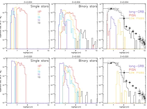
For any system with a core-collapse supernova we es-timate the supernova category as type IIP, II-other, Ib and Ic. We identify the supernova types as described in Eldridge et al.(2011) andEldridge et al.(2013). If the
mass of hydrogen in the star is greater than 10−3M
⊙ then we have a type II supernova. If the total mass of
hydrogen is greater than 1.5 M⊙ and the ratio of
hydro-gen mass to helium mass in the prohydro-genitor is greater than 1.05 we have a type IIP. When the hydrogen mass is less than 10−3M
⊙ a type Ib/c supernova occurs. If
more than 10% of the ejecta mass is helium then the supernova is assumed to be a type Ib, otherwise it is Ic. This leads to roughly twice as many Ib as Ic supernovae which is in agreement with the most recent attempt to accurately determine this ratio (Shivvers et al.,2017).
We also determine whether an event is likely to gen-erate a Gamma-ray Burst (GRB) or Pair-Instability Su-pernova (PISN). For a long-GRB the star must have ex-perienced QHE and have a remnant mass greater than
3 M⊙. Note that this is only one possible pathway for
GRBs and limits their presence in our rate estimates to lower metallicities. Some type Ic supernovae arising from non-QHE systems also likely generate GRBs but we do not account for these. For PISN we apply mass limits from Heger & Woosley(2002) as detailed above. Finally any progenitor with a final mass between 1.5
and 2 M⊙ is identified as a low-mass progenitor with
an uncertain outcome. These events may be faint and
rapidly evolving, as described by Moriya & Eldridge
(2016).
We also estimate the type Ia thermonuclear super-nova rate by two channels, first selecting out white dwarfs that begin with a mass below the Chandrasekhar limit but then reach or exceed this mass due to binary mass transfer. Second, we count double white dwarf bi-naries that merge due to gravitational radiation with the merger time calculated assuming circular orbits and the analytic expressions ofPeters(1964). Our resultant rates are highly approximate and we do not consider them rigorous or precise but include them for complete-ness. We caution that these should be used with care, and in future we may refine our type Ia models further for comparison with other predictions and observational data.
2.2 The Population Synthesis
2.2.1 Binary distribution parameters
[image:11.612.333.553.69.579.2]In the population synthesis the individual stellar mod-els are combined together to make a synthetic stellar
Table 1BPASS v2.1 input parameter ranges for binary populations
Parameter Permitted Values
Primary Masses 68 values from M1=0.1, 0.2, 0.3, 0.4, 0.5, 0.6, 0.7, 0.8, 0.9, 1, 1.1, 1.2, 1.3, 1.4,
1.5, 1.6, 1.7, 1.8, 1.9, 2, 2.1, 2.3, 2.5, 2.7, 3, 3.2, 3.5, 3.7, 4, 4.5, 5, 5.5, 6, 6.5, 7, 7.5, 8, 8.5, 9, 9.5 10, 11, 12, 13, 14, 15, 16, 17, 18, 19, 20, 21, 22, 23, 24, 25, 30, 35, 40, 50, 60, 70, 80, 100, 120, 150, 200 and 300 M⊙.
Primary Mass Ratios 9 values with M2/M1= 0.1, 0.2, 0.3, 0.4, 0.5, 0.6, 0.7, 0.8, 0.9
Secondary Masses 46 values from M2= 0.1, 0.2, 0.3, 0.4, 0.5, 0.6, 0.8, 1, 2, 3, 4, 5, 6, 7, 8, 9, 10,
11, 12, 13, 14, 15, 16, 17, 18, 19, 20, 21, 22, 23, 24, 25, 30, 35, 40, 50, 60, 70,
80, 100, 120, 150, 200, 300, 400 and 500 M⊙.
Compact remnant masses 31 values from log(Mrem,1/M⊙) = -1, -0.9, -0.8, -0.7, -0.6, -0.5, -0.4, -0.3, -0.2, -0.1, 0, 0.1, 0.2, 0.3, 0.4 ,0.5, 0.6, 0.7, 0.8, 0.9, 1, 1.1, 1.2, 1.3, 1.4, 1.5, 1.6, 1.7, 1.8, 1.9 and 2.
Period Distribution 21 initial periods from log(P/days) = 0, 0.2, 0.4, 0.6, 0.8, 1, 1.2, 1.4, 1.6, 1.8,
2, 2.2, 2.4, 2.6, 2.8, 3, 3.2, 3.4, 3.6, 3.8, 4.0
Stellar Ages Output ages from log(Age/yrs) = 6.0 to 11.0 (1 Myr to 100 Gyr)
Metallicity Mass Fractions Z = 10−5, 10−4, 0.001, 0.002, 0.003, 0.004, 0.005, 0.006, 0.008, 0.010, 0.014,
0.020 (Z⊙), 0.030, 0.040
Initial Mass Functions 7 different mass functions - fiducial version: has an IMF slope of -1.30 from
0.1 to 0.5M⊙, and a slope of -2.35 from 0.5 to 300M⊙. We have variations
with other upper mass slopes of -2.00 and -2.70 and also versions with the
upper mass of 100M⊙. Our final alternative has a slope of -2.35 from 0.1 to
100Modot
Stellar Atmospheres BASELv3.1 (logg=−1 to 5.5, log(T /K) = 2000 to 50000 and log(Z/Z⊙) =
−3 to 0.5. For metallicities below this minium we use v2.2 that extends to
log(Z/Z⊙) =−3.5.)
PoWR (We use the SMC and LMC, WN grids with Xsurface = 0.4, 0.2 and
0. For the Galaxy we use the WN grids withXsurface= 0.5, 0.2 and 0. At all
metallicities we use the Galactic WC grid.)
population which can be observed and compared to ob-servations of the real Universe. Together with the mod-els described above we need to know the distribution of initial parameters required to create the population. The three main parameters are the initial mass func-tion (IMF), the initial period distribufunc-tion and the initial mass-ratio distribution. Each population is generated at a single initial metallicity. For our fiducial models we
base our IMF on Kroupa et al. (1993) with a
power-law slope from 0.1 to 0.5 M⊙ of -1.30 which increases
to -2.35 above this. The power law slope extends to a
maximum initial stellar mass of 300 M⊙, although we
note that due to mergers stars more massive than this can form in our binary populations. Our most massive
stars have masses up to 570 M⊙although these are very
rare systems. In addition to this standard model we also calculate models with two different upper IMF slopes of -2.00 and -2.70, as well as varying the upper maximum
initial stellar mass to 100 M⊙. Finally we calculate a
model set with a constant IMF slope of -2.35 from 0.1
to 100 M⊙(the standardSalpeter(1955) IMF), for
com-parison with previous work.
For the binary populations, we assume a flat distribu-tion in initial mass ratio and log-period in all our mod-els. The result of this is that while all of our stars are technically part of a binary population, in many cases the stars evolve as isolated individuals and are never close enough to interact. The actual interacting binary fraction will depend on the physical size of stars at dif-ferent ages relative to their Roche lobes, and thus on mass and metallicity. Our upper period limit of 10000 days has been chosen so that about 80% of massive stars
(M &5 M⊙) interact, as shown in Figure1. From 5M⊙
to 0.7M⊙this fraction decreases to about 50%. At lower
masses the separation of the orbits with a 1 day min-imum is too wide for stars to interact within the age of the Universe. At Solar metallicity, many of the most massive (M ∼100 M⊙) stars also avoid interactions due
to strong mass-loss in stellar winds.
Observational constraints on these numbers are un-certain but our estimates of massive star interaction are comparable to the 70% estimated for O stars by Sana et al. (2012). On the other hand, the flat distri-butions are probably over-simplistic. As discussed by De Marco & Izzard (2017) binary parameters (includ-ing the binary fraction) vary with initial mass. While nearly every massive star is in a binary, the binary frac-tion drops to 20% at lower initial masses below a Solar mass, but the precise binary fraction as a function of stellar mass remains poorly constrained in the
litera-ture. In the Milky Way, Sana et al. (2012) found that
the observed period distribution is slightly steeper than flat, with a bias towards more close binary systems for
O stars. However Kiminki & Kobulnicky(2012) found
a flatter period distribution in the Cygnus OB2 associa-tion that is consistent withÖpik(1924)’s law, although
their results did also suggest a slight preference for short
period systems as well. The most recent study by Moe
& Di Stefano(2017) has quantified the period and mass ratio distribution in an extensive compilation of previ-ous works, and finds a slightly different period and mass ratio distribution to that we use. We intend to modify our input distributions accordingly in a future version of BPASS.
The uncertainty in assumed period distribution is de-generate with uncertainties in the assumed model to handle Roche lobe overflow, common envelope evolu-tion, tides and other binary specific processes. Hence we adopt this simple approach based on the well-studied massive star population (Sana et al.,2012). If required, it is possible to simulate the effect of more complex pop-ulations and binary distributions by varying the mix be-tween our single star and binary populations with age (since stars of different initial masses dominate in differ-ent time bins).
We note that, because we assume orbits are circular, our closest observational comparison will be with the semi-latus rectum distribution not the period
distribu-tion. As shown by Hurley et al. (2002), the outcome
of the interactions of systems with the same semilatus rectum is almost independent of eccentricity. This is equivalent to assuming that systems are circularised by tidal forces before interactions occur. We only include tides in our evolution models when a star fills its Roche lobe as this can move the system into CEE if there is not enough angular momentum in the orbit to spin up the primary. We assume tidal forces are strong and the star’s rotation quickly synchronises with the orbit. This is of course an approximation and there are recent stud-ies have begun to explore how mass transfer may be different in eccentric systems (e.g.Sepinsky et al.,2007; Bobrick et al.,2015;Dosopoulou & Kalogera,2016a,b). However we note that the BPASS stellar models have been successfully tested to see if they can reproduce an observed binary system with a slight eccentricity even after mass transfer (Eldridge,2009).
2.2.2 Binary evolution treatment
We combine all the primary star models together accord-ing to these distributions. We then must consider how to account for the secondary stars. We pick out the stars that explode in supernovae by and estimate the
rem-nant mass as described in Section 2.1.3. For remnants
less than 3 M⊙ we assume that the remnant receives a
kick taken at random from a Maxwell-Boltzmann dis-tribution withσ= 265 km s−1 (seeHobbs et al.,2005).
For remnants more massive than 3 M⊙ we assume the
star has a kick that is reduced by a factor of the
rem-nant mass divided by 1.4 M⊙, assuming that the kicks
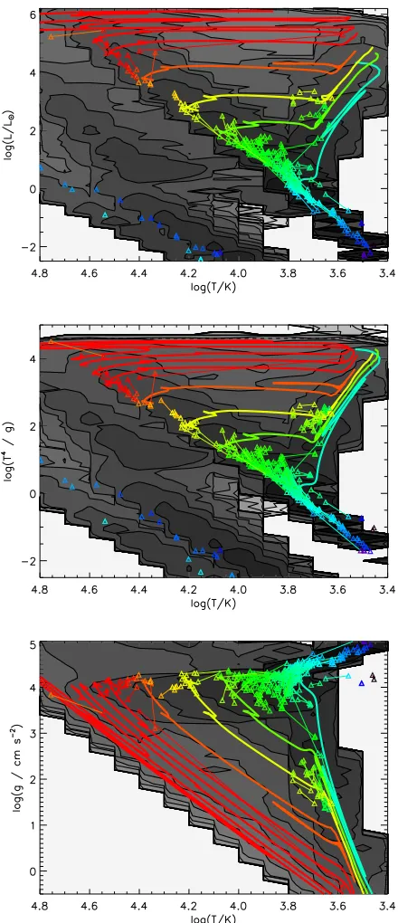
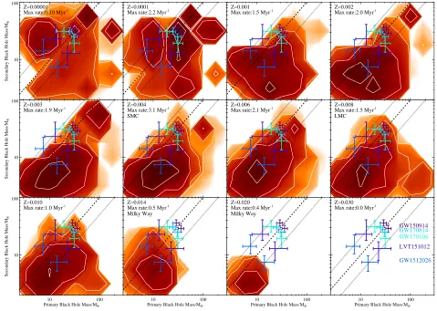
Figure 9.Eclipsing binaries overplotted on evolution tracks for our binary models (greyscale, indicating the range of outcomes for a given initial mass). The observed population of eclipsing binaries are overplotted as small symbols, with lines linking bi-nary companions, coloured by metallicity. We show distributions for key parameters. The observational data is mainly taken from
Southworth(2015) and supplemented by VV Cephei, WR20a and
γ-Velorum, as well as the white dwarf sample of Parsons et al.
(2017) as detailed in the text.
(Mandel,2016). We note that we have also investigated other models of neutron-star kicks but have not yet in-cluded these in the released BPASS models (seeBray & Eldridge,2016).
If the binary is disrupted then the companion star is modelled as a single star in its further evolution. Con-versely if it remains bound then the post-supernova or-bit is calculated, circularized and a secondary model of a star orbiting a compact remnant is used to represent its future evolution. Eventually if a second supernova oc-curs the same process is repeated so that the parameters of double-compact remnant binaries can be estimated. Note that the secondary may still undergo supernova, even if the primary does not: this possibility is followed and these later events are also considered.
We also check in our models for rejuvenation of the secondary stars. If a secondary star accretes more than
5% of its initial mass and it is more massive than 2 M⊙
then the star is assumed to be spun-up to critical rota-tion and is rejuvenated due to strong rotarota-tional mixing. That is, it evolves from the time of mass transfer as a more massive, zero-age main sequence star (this is sim-ilar to the method used byVanbeveren et al.,1998). At high metallicities we assume that the star quickly spins down by losing angular momentum in its wind so that there are no further consequences for its evolution.
How-ever with weaker winds at lower metallicity,Z≤0.004,
we assume that the spin down occurs less rapidly and so the star remains fully mixed throughout the main-sequence and burns all its hydrogen to helium. We as-sume the star must have an effective initial mass after accretion>20 M⊙for this evolution for occur, based on
the work ofYoon et al. (2006). We note that we have
discussed the importance of these quasi-homogeneously
evolving (QHE) stars in greater detail inEldridge et al.
(2011);Eldridge & Stanway (2012) andStanway et al.
(2016) showing there is strong observational evidence
that they exist. We only consider QHE that arises from mass transfer, however, and do not yet include it in tidal interactions as done byMandel & de Mink(2016) and Marchant et al. (2016). In such a scenario, stars can be spun up by tidal forces acting between two stars in orbital periods of the order of a day, leading to both stars experiencing QHE; this is not yet implemented in BPASS.
2.2.3 Binary Mass Function as a function of age We present some fundamental results from our
popula-tions in Figures3 and4which concern the mass in the
stars at different different stellar population ages. Fig-ure3shows that from an initial 106M
SN occurs. This leads to an offset between the binary and single star populations which persists until late times. Higher metallicity populations retain more mass at late times. This is because the higher metallicity stars have longer lifetimes due to being less compact with lower central temperatures so burning through their nu-clear fuel takes a longer time. Although at early times the far stronger winds of high metallicity stars means more mass is lost at early times for the higher metallic-ity population. After this, the stars will evolve along the lower-mass pathways at an appropriate rate. The net ef-fect of this is to lead to longer total stellar lifetimes and so a delay in the death of the stars and formation of remnants. By the age of 1 Gyr, a Solar metallicity star-burst will have lost 37% (39%) of its initial mass in the binary (single) star evolution case. This is towards the upper end of the “return fractions” of material to the ISM ofR∼0.4 for aChabrier(2003) IMF andR∼0.3
for a Salpeter (1955) IMF found by Madau &
Dickin-son(2014). At 20% of Solar metallicity, both binary and
single star return fractions increase by∼2%.
Figure4illustrates this effect in greater detail, show-ing how the stellar mass functions vary with age at the same two metallicities. In both cases, due to rapid merg-ers of the most massive membmerg-ers of a stellar population, binary populations can have more massive stars than were initially assumed and these can retain mass for longer. At late times the most massive star is always beyond that expected from single-star populations: the phenomenon that leads to the observation of “blue strag-glers” in globular cluster populations. The mass of the most massive star is greater at late times in high metal-licity populations, even though at early times the mass of individual stars rapidly decreases due to the stronger mass-loss.
We note here that beyond approximately 3 Gyrs our current models predict a population of more massive stars than would be expected. These are more than twice the maximum mass for a single star population at this age. These are systems where the primary evolved to a white dwarf after rejuvenating it’s companion star. Our simple method of estimating the rejuvenation age currently uses the age at the end of the model rather than the time of the mass transfer. While this is ade-quate if the primary explodes in a supernova it is not for the case where our models include the time on the white dwarf cooling track.
2.3 Stellar Atmospheres and Spectral Synthesis
While the stellar models described above contain a large amount of detail about the structure, physical condi-tions (e.g. temperature, surface gravity) and evolution of stars in a population they provide relatively limited information about their appearance. This is because the
physics of stellar atmospheres comprises a second mod-elling challenge that can be as complex and difficult to calculate as a stellar evolution model. The compu-tational time to calculate a model atmosphere for one set of surface conditions can be the same as the time to calculate the entire evolution of a single stellar model. Therefore some compromise must be found in connect-ing the evolution and atmosphere models. Some authors (e.g.Rix et al.,2004;Groh et al.,2014;Topping & Shull,
2015) have calculated sets of atmosphere models for
spe-cific phases of evolution of their stellar models and in-terpolate between these. Our solution has been to use pre-calculated grids of atmospheres that we then match to our evolution models to predict their luminous out-put spectrum. The exception is for extreme cases where no appropriate atmosphere grid is extant: we have cre-ated a new set of atmosphere spectra for hot OB stars from existing tools. We detail these grids in section2.3.2 below.
2.3.1 Existing Model Grids
Our base atmosphere models are those of the BaSeL v3.1 library (Westera et al., 2002). This is a set of
at-mosphere models that extend over a large range of logg,
logTeff and metallicity. We interpolate between models
to predict the spectrum of each star generated by our evolution code. This version only extends over metallici-ties from [Fe/H]=-2.0 to 0.5. We therefore at our lowest
metallcities use the slightly older v2.2 grid of Lejeune
et al. (1998) that extends down to [Fe/H]=-3.5. We supplement these with Wolf-Rayet (WR) stellar
atmosphere models from the Potsdam PoWR group3
(Hamann & Gräfener, 2003; Sander et al., 2015). We only use WR spectra once the surface hydrogen abun-dance drops below 40% and the surface temperature
is above log(T /K) = 4.45. A key change implemented
in BPASSv2.0 and v2.1 is that there are now different metallicity nitrogen-dominated (WN) Wolf-Rayet atmo-spheres available (Todt et al., 2015). In our previous work (such as Eldridge & Stanway, 2009), only Solar metallicity were available and we artificially reduced the line luminosities of these models at lower metallicites. We now use the closest metallicity WN models to the
stellar models being considered. When Z ≥0.0095 we
use the Solar PoWR models, below this limit we use
their LMC models and when Z <0.0035 we use their
SMC models. For WC (i.e. carbon-dominated) Wolf-Rayet stars there are still only Solar metallicity models available, but we have not altered these spectra in any way in our current models, using the Solar models at all metallicities. This may lead to slight overestimates in the strength of carbon WC features in low metallicity spectra but the abundances in the stellar atmospheres during the WR phase are relatively insensitive to the
3
Table 2 WM-Basic input parameter ranges for new O star grids
Luminosity Class Parameter Calculated Values
Dwarfs logg 4.0 and 4.5
T/kK 50.0, 45.7, 42.6, 40.0, 37.2, 34.6, 32.3, 30.2, 28.1, 26.3 and 25.0
Supergiants logg 3.88, 3.73, 3.67, 3.51, 3.40, 3.29, 3.23, 3.14, 3.08, 2.99 and 2.95
T/kK 51.4, 45.7, 42.6, 40.0, 37.2, 34.6, 32.3, 30.2, 28.1, 26.3 and 25.0
initial metallicity (which has a larger effect on mass-loss rate). This will be modified as as further PoWR models become available. We switch to the WC models when there is no surface hydrogen and the helium mass fraction drops below 70%.
As in Eldridge & Stanway (2009) we add in an
excess He II flux for massive Of stars as suggested by Brinchmann et al. (2008) since these are under-represented in atmosphere models. For non-WR stars with a surface temperature above 33000K and when logg ≤ 3.676 log(T /K)−13.253, we increase the He
II stellar wind lines at 1640Å and 4686Å by 520 L⊙ and
33.8 L⊙ respectively. Due to the rarity of these cases,
we find this has a minimal effect on the predicted pop-ulation line fluxes. Interestingly,Crowther et al.(2017) have studied He II emission from massive stars in the Tarantula Nebula and report a very high equivalent width for a young stellar population. We note that with our current prescription as described above, our v2.1 models produce a comparably high equivalent width at slightly older (but similar ages), see Section6.1and
Fig-ure28below.
2.3.2 New O star models
In previous distributions of BPASS models, we supple-mented the above with a set of O star models
gener-ated using the WM Basic code by Smith et al.(2002).
We have now recalculated this grid, and extended it, as
summarised in Table24
For BPASS v2.1 models we have created new
WM-Basic (Pauldrach et al., 1998) models based upon the
grid determined by Smith et al. (2002). The key
dif-ferences are that we have extended the metallicity cov-erage and also added a new sequence of models with a higher surface gravity to better match the evolution code predictions. We have kept the range of
tempera-tures the same (25-50 kK) but now added a grid ofhigh
gravitystars with logg= 4.5 (c.f. 4.0 in the earlier grid). This is because we noticed that on the zero-age main-sequence many of our O stars had gravities higher than 4.0 which has a significant effect on the strength of some stellar lines. At low metallicities our QHE models also increase their surface gravity as they evolve with the stars shrinking as helium is mixed to the surface and the mean-molecular weight increases. Therefore these new
4
These new models are the first of the two main differences between v2.0 and v2.1.
models are important for predicting the correct spec-trum.
We also calculate models at every metallicity we con-sider in BPASS rather than simply interpolating be-tween fixed points as before. The key benefit is that we now have spectra at the lowest metallicities when
Z = 10−5 and 10−4, where the influence of these
mas-sive stars on the synthetic spectrum is strongest. These are beyond the range for which observational validation data is available for stellar atmospheres and so consti-tute a theoretical extrapolation from better constrained atmospheres at higher metallicity. However incorporat-ing these gives greater predictincorporat-ing power for stellar pop-ulations at these extreme metallicities.
We have made these models available on the BPASS website and they have already been used in other pub-lished works (e.g.Byler et al.,2017). We note that only the inclusion of the higher gravity models leads to any significant differences in model outcomes. We find that the ionizing flux predictions at low metallicites decrease by about 0.1 dex, but that the far-ultraviolet luminosity of a population increase by a similar amount (see figure
35 later). This is because the QHE evolution models
have more correct atmospheres. These stars evolve to hotter temperatures as they burn hydrogen to helium. These models also allow us to predict O V 1039Å lines at very young ages that are comparable to those found in observations (A. Runnholm, private communication).
2.4 BPASS model outputs
2.4.1 Spectral Energy Distributions
The basic output of BPASS is a set of moderately high resolution model spectra, gridded from 1 to 100,000Å in 1Å bins and measuring total flux in each wavelength
bin in units of L⊙ (i.e. producing a spectrum of Fλ
in L⊙/Å spanning from the extreme-ultraviolet to
far-infrared wavelengths). These are generated for stellar
population ages of 1 Myr to 100 Gyr5 in increments of
∆ log(age/yr) = 0.1 where this age is taken relative to the onset of star formation, assuming a co-eval stellar
population of total mass 106M
⊙. Examples are shown
in Figure5and6, illustrating the optical-infrared spec-tral energy distributions as a function of age and the
5
extreme ultraviolet as a function of metallicity and bi-nary evolution respectively.
In Figure7we show a direct comparison between the
simple stellar population models (i.e. co-eval starbursts) produced by different stellar population synthesis codes at Solar metallicity and allowed to evolve over time. In three panels, BPASS single star models are compared to the closest available matching models in metallicity, age and initial mass function from publicly available synthesis codes. Perhaps the most direct comparison is
between BPASS and the Starburst99 models (Leitherer
et al., 1999, 2014, hereafter S99), both of which were originally designed and optimised for young starbursts. The S99 models shown here were generated using the non-rotating Geneva 2012/2013 stellar model set and a broken power law IMF with slopes matching our default
IMF but with a maximum stellar mass of 100 M⊙.
We also compare against two SPS codes designed pri-marily for modelling galaxies. The GALAXEV models ofBruzual & Charlot(2003, hereafter BC03) are widely used for modelling mature galaxies and specifically we compare against the galaxy templates used to classify
galaxies in the Sloan Digital Sky Survey by Tremonti
et al. (2004). These use a Chabrier (2003) IMF and are built on the Geneva and Padova single star stellar evolution models, combined with a large library of semi-empirical template spectra and additional atmosphere
models calculated using the BaSeL code (Westera et al.,
2002). TheMaraston(2005, hereafter M05) models were
designed to confront the thermally pulsating AGB stage in more detail than previous models and use a prescrip-tion for fuel consumpprescrip-tion to determine the contribuprescrip-tion of post-main sequence stars and their role in determin-ing the near-infrared colours of galaxies. They employ the Cassisi stellar evolution tracks (Cassisi & Salaris, 1997;Cassisi et al.,2000), BaSeL atmospheres (Lejeune et al.,1998) and aKroupa(2001) broken power law IMF similar to ours (with an upper power law slope of -2.30
where we use -2.35, and a maximum mass of 100 M⊙).
As the figure demonstrates, the BPASS single star models are very similar to all three other synthesis mod-els at ages of<1 Gyr and in the ultraviolet, where the models are dominated by massive stars. The BC03 mod-els are slight outliers, appearing redder at very young ages (<10 Myr) than any of the other model sets. Our single star models remain similar to the output of other codes at a matching age through the blue optical bands, with subtle differences in the IMF and evolutionary timescales assumed for the most massive stars by dif-ferent evolution codes leading to our single star models being slightly bluer than S99 and M05 models but
red-der than BC03 models at ages of∼10-100 Myr.
BPASS models begin to diverge significantly from the other model sets in the red-optical and longwards at stel-lar population ages of more than a few times 100 Myr. At these ages, the light from our single star populations
are dominated by evolved massive stars, primarily AGB stars, whose molecular line features are clearly visible in the composite SED. Perhaps unsurprisingly our mod-els are most similar in the infrared to the M05 modmod-els, which are also heavily influenced by the AGB phase, but we see a stronger effect still. Realistically, this compari-son suggests that AGB stars are over-represented in our co-eval single star populations (either in terms of num-ber or luminosity) at ages>1 Gyr. In our favoured bi-nary models (shown in the fourth panel of Figure7), the number of AGB stars in a population is suppressed by the effect of binary interactions, but these interactions also keep the spectra rather bluer than those seen in other stellar population synthesis models at late times. We note that extreme caution should be applied when
us-ing this version of BPASS in the red at ages >1Gyr as
a result; we return to this point in section7.10.
2.4.2 Released Data Products
The spectral energy distributions described above for co-eval simple stellar populations form the core of the BPASS v2.1 data release. Composite (i.e. non-co-eval) stellar populations are not provided as a part of our standard release but can be constructed by assuming
a star formation history (see section6.2). The simplest
case is a population forming stars continuously at a con-stant rate. Here the only potential difficulty lies in deal-ing with logarithmically spaced time intervals in the models since the total number of stars to be added to the composite spectrum depends on the width of the interval. Stars contributing to the first time bin (at log(age/years)=6.0) include all members of the popu-lation up to age 106.05, the second bin stars in the age
range 106.05to 106.15 years and so forth.
We calculate magnitudes for individual stellar mod-els and for our synthetic populations in the standard
U BV RIJHK filters, as well as ugriz SDSS filters,
F U V(1566Å),N U V(2267Å) fluxes and several HST
op-tical filters at each step. Additionally we calculate the production rate of ionizing photons based on the ex-treme ultraviolet flux since this is strongly affected by
both binary evolution and metallicity (see Figure6and
Stanway et al.(2016)).
Given that our population synthesis tracks all stages of stellar evolution, we are also able to produce corre-sponding rates of supernovae (separated by type) and information on the compact remnant population and stellar class distribution at each time step.
1. Stellar Model Outputs:
(a) Binary stellar models with photometric colours
(b) New OB stars atmosphere models 2. Stellar Population Outputs (all versus age):