Adapting the Gibbs sampler

(1)

warwick.ac.uk/lib-publications

A Thesis Submitted for the Degree of PhD at the University of Warwick

Permanent WRAP URL:

http://wrap.warwick.ac.uk/108829

Copyright and reuse:

This thesis is made available online and is protected by original copyright.

Please scroll down to view the document itself.

Please refer to the repository record for this item for information to help you to cite it.

Our policy information is available from the repository home page.

(2)

Adapting the Gibbs Sampler

by

Cyril Chimisov

Thesis

Submitted to the University of Warwick

for the degree of

Doctor of Philosophy

Department of Statistics

(3)

Acknowledgments

First, I would like to express my genuine gratitude to Dr Krys Latuszy´nski and

Prof Gareth Roberts. Without their guidance and patience, it would not have been

possible to complete this dissertation. It was a great pleasure to have all the fruitful

and encouraging discussions, which have led to the development of ideas described

in the present work.

I also owe a great deal of gratitude to Murray Pollock, Christian Robert and Matt

Moores, with whom I had numerous conversations, which helped me comprehend

a large chunk of the Bayesian world. I would also like to thank every member

of the Algorithms, Simulations, and Machine Learning reading groups, and, more

generally, everyone at the Department of Statistics for creating the dynamic and

stimulating environment.

Special thanks to Daniel, Ellie, Neil, Rodrigo, Te-Anne and my office mates who

have shaped my life for the much better.

It would not be possible to stay concentrated and motivated throughout the PhD

years without my caring and supportive partner Lana. Last but not the least, I

would like to thank my mother, who has given me more than I can ever give back.

I would also like to acknowledge the Engineering and Physical Sciences Research

Council (grant number EP/M506679/1) and the University of Warwick for the

(7)

Many thanks to Kengo Kamatani and Anthony Lee for taking their time to

thor-oughly read and examine my work, and also for making useful suggestions to improve

(8)

Declarations

I hereby declare that the present thesis has been written by myself and that the

work has not been submitted for any other degree or professional qualification. All

the content was obtained by legal means. Every effort has been made to indicate

(9)

Abstract

In the present thesis, we close a methodological gap of optimising the ba-sic Markov Chain Monte Carlo algorithms. Similarly to the straightforward and computationally efficient optimisation criteria for the Metropolis algorithm accep-tance rate (and, equivalently, proposal scale), we develop criteria for optimising the selection probabilities of the Random Scan Gibbs Sampler. We develop a general purpose Adaptive Random Scan Gibbs Sampler, that adapts the selection proba-bilities, gradually, as further information is accrued by the sampler. We argue that Adaptive Random Scan Gibbs Samplers can be routinely implemented and sub-stantial computational gains will be observed across many typical Gibbs sampling problems.

(10)

List of Algorithms

1 Metropolis-Hastings . . . 3

2 Gibbs sampler . . . 6

3 Metropolis-within-Gibbs. . . 7

4 AirMCMC Sampler . . . 15

5 Adaptive Random Scan Gibbs Sampler (general idea) . . . 27

6 Subgradient optimisation algorithm . . . 29

7 Adaptive Gibbs Sampler based on subgradient optimisation method (not implementable) . . . 30

8 Projection on ∆ε_s . . . 31

9 Adaptive Random Scan Gibbs Sampler (final version) . . . 35

10 Random Walk Metropolis-within-Gibbs . . . 36

11 Adaptive Random Walk Metropolis-within-Gibbs . . . 37

12 Adaptive Random Walk Metropolis within Adaptive Gibbs . . . 37

13 Modified AMCMC . . . 41

14 Adaptive Random Scan Gibbs Sampler (ergodic modification) . . . . 44

15 Parallel versions of ARSGS and ARWMwAG . . . 58

16 AirRWM . . . 72

17 Modified AirMCMC Sampler . . . 82

18 Randomised AirMCMC Sampler . . . 87

(11)

Abbreviations

• AirMCMC – Adapted Increasingly Rarely Markov Chain Monte Carlo

• ACF – Autocorrelation Function

• AMCMC – Adaptive Markov Chain Monte Carlo

• ARSGS – Adaptive Random Scan Gibbs Sampler

• ARWM – Adaptive Random Walk Metropolis

• ARWMwAG – Adaptive Random Walk Metropolis within Adaptive Gibbs

• ARWMwG – Adaptive Random Walk Metropolis within Gibbs

• CLT – Central Limit Theorem

• DUGS – Deterministic Update Gibbs Sampler

• HMC – Hamiltonian Monte Carlo

• KAMH – Kernel Adaptive Metropolis-Hastings

• LLN – Law of Large Numbers

• MALA – Metropolis Adjusted Langevin Algorithm

• MCMC – Markov Chain Monte Carlo

• MSE – Mean Squared Error

(12)

• PHM – Poisson Hierarchical Model

• RSGS – Random Scan Gibbs Sampler

• RWM – Random Walk Metropolis

• RWMwG – Random Walk Metropolis within Gibbs

• SLLN – Strong Law of Large Numbers

• TMVN – Truncated Multivariate Normal

(13)

Chapter 1

Introduction

1.1 Markov Chain Monte Carlo

Markov Chain Monte Carlo (MCMC) methods are a class of tools to sample from a generic probability distribution which are widely used in virtually any field where one needs to deal with uncertainty (see e.g.,Gelman et al.[2004],Liu[2001],Robert and Casella [2004] for various examples). These methods are of particular interest in Bayesian statistical inference, where one has to estimate a model parameter as an integral with respect to a posterior distribution. More generally, in many scientific problems we are interested in computing

π(f) = Z

f(x)π(dx)

for various measurable functionsf (see, e.g., Chapter 1 of Liu[2001]).

An elegant Monte Carlo method to estimate integralsπ(f) was introduced by Metropolis and Ulam[1949]. The method is based on the idea that by generating a number of independent samples{Xi}iN=0−1 from the distributionπ, the integralπ(f)

can be estimated as

ˆ

πN(f) := 1

N

N−1

X

i=0

f(Xi). (1.1)

By the Law of Large Numbers, ˆπN(f) converges to π(f) almost surely, if the lim-iting integral exists. However, the distribution of interest often has a complicated structure so that the direct sampling fromπ is not feasible.

(14)

Monte Carlo methods. An MCMC algorithm runs a Markov chain that converges toπ. Of course, we expect the Markov chain to be implementable on a computer. The output of the chain{Xi}Ni=0 can then be used in the same manner as the Monte

Carlo samples, i.e., we could compute (1.1) in order to estimateπ(f).

Due to the lack of computational power and limited availability of computers at the time, it took another few decades before publication of the seminal paper by Hastings[1970], who generalised the ideas ofMetropolis et al.[1953] in an algorithm now known as the Metropolis-Hastings algorithm. A further push towards popu-larity of the MCMC methods has been done by Geman and Geman [1984], who developed the Gibbs Sampler which is the basic algorithm to deal with Hierarchical models (see, e.g., Gelman et al. [2004]). The interested reader can find a detailed historical background inRobert and Casella [2011].

There is a wide variety of MCMC algorithms available for users’ needs. The present thesis focuses on two of the aforementioned frameworks, namely, the Metropolis-Hastings and Gibbs Sampler. As we shall show below, many of cur-rently popular algorithms fall into the Metropolis-Hastings framework, such as Ran-dom Walk Metropolis (RWM), Metropolis-adjusted Langevin Algorithm (MALA), or Hamiltonian Monte Carlo (HMC). All of these algorithms have parameters that need to be chosen by the user. Moreover, any of them can be interlaced with the Gibbs Sampler into the Metropolis-within-Gibbs Sampler, which altogether provides users with plenty of algorithms to choose from. Below we describe the Metropolis-Hastings and Gibbs Sampler frameworks in greater detail.

1.1.1 Metropolis-Hastings framework

We assume that the reader is familiar with basic Markov Chain theory on general state spaces and refer to Meyn and Tweedie [2009] for the main definitions and results. The basic concepts of the MCMC theory can be found in Roberts and Rosenthal[2004]. Having this remark in mind, we outline the Metropolis-Hastings framework below.

Letπ be a probability distribution of interest on a state spaceX with count-ably generatedσ−algebra. Often,X is a subset of ad-dimensional Euclidean space

Rd. Let Q(x,·) be essentially any Markov kernel on X. For practical reasons, Q should be chosen so that for anyx∈ X, it is possible sample from Q(x,·).

We assume that both π and Q(x,·) have densities with respect to (w.r.t.) some reference measureϕonX (usually,ϕis the Lebesgue measure onRd). Without causing ambiguity, let π(x) and q(x, y) denote the corresponding densities.

(15)

a Markov chain using the kernelQwith an additionalacceptance-rejectionprocedure at each iteration, that ensuresπis a stationary distribution of the underlying Markov chain.

Algorithm 1:Metropolis-Hastings

Set some initial values forX0 ∈ X;n:= 0.

Beginning of the loop

1. Sample a proposalY ∼Q(Xn,·);

2. Compute acceptance ratioα=α(Xn, Y) = min

(

1, π(Y)q(Y,Xn)

π(Xn)q(Xn,Y)

) ;

3. With probabilityα accept the proposal and set Xn+1 =Y, otherwise,

reject the proposal and setXn+1 =Xn;

4. n:=n+ 1;

Go toBeginning of the loop

The target distribution π is only utilised when computing the acceptance ratio α in Step 2. Since α involves a ratio of π at two points, the user needs to know the density π only up to a normalising constant. The acceptance ratio α is specifically constructed to ensure that the algorithm produces a reversible chain w.r.t. π and thus, implying that π is a stationary distribution of the chain (see Propositions 1 and 2 ofRoberts and Rosenthal [2004]).

It is possible to use a different version of the acceptance ratio in Step 2

(see an algorithm by Barker[1965] and a discussion by Tierney[1998]) but for the purpose of present thesis we restrict ourselves to the Metropolis-Hastings framework of Algorithm1. Many of the well-known popular algorithms fall into this framework:

• Random Walk Metropolis (RWM). Here the kernel density has a property

q(x, y) =q(x−y). OftenQ(x,·)∼N(x,Σ) is chosen to be a normal distribu-tion centred atx with some user-defined covariance structure Σ.

• Metropolis-adjusted Langevin Algorithm (MALA). Here we assume that the support of the target distribution π is the Euclidean space X =Rd and that logπ exists and differentiable. The proposal is generated using a single step of the discretised Langevin dynamics (see,Roberts and Tweedie [1996]):

Y ∼N Xn+σ2/2∇logπ(Xn), σ2Id

, (1.2)

(16)

the identity matrix of dimensiond.

• Hamiltonian Monte Carlo (HMC). The algorithm is based on the discretisation of Hamiltonian dynamics for a target distribution π supported on Rd (see Duane et al. [1987], Neal [2011], Hoffman and Gelman [2014]). We assume that logπ exists and differentiable. The Markov chain (Xn, rn) corresponding

to the algorithm evolves on the extended space R2d and has a stationary distribution π×N(0, Id), i.e., a product distribution of π and the standard

multivariate normal distribution. The proposal (Y, r) is generated in three steps:

1. Generater∼N(0, Id), setY =Xn;

2. For user-defined constantsL∈N, ε >0, evolve (Y, r) L times using the leapfrog integrator:

r:=r+ε

2∇logπ(Y);

Y :=Y +εr;

r:=r+ε

2∇logπ(Y);

3. Setr:=−r.

It turns out that the corresponding density of the proposal is symmetric, i.e.,

q(x, r),(˜x,˜r) = q(˜x,r˜),(x, r), so that the acceptance ratio in Step 2 of

Algorithm1 simplifies to π(Y) exp(−r 2_/₂₎

π(Xn) exp(−rn2/2).

Remark. The presented MALA and HMC samplers are not in their most generic form. A non-isotropic and non-constant diffusion matrix can be used for MALA Roberts and Stramer [2002], Stramer and Tweedie [1999], i.e., the proposal co-variance matrix can take the form M =M(Xn) in (1.2); a non-isotropic proposal

N(0, M) can be used in Step 1of the HMCNeal [2011]. For further discussions we refer the reader toGirolami and Calderhead[2011].

From practical point of view, it is important to have a guarantee of conver-gence for the MCMC algorithms. The basic type of converconver-gence for Markov chains is theconvergence in distributionortotal variation convergence.

Definition. We say that the MCMC is ergodic if it converges in distribution, i.e.,

lim

(17)

where L(Xn|X0 = x) is the distribution law of the chain at iteration n started at

location x, and for a signed measure ν on X, kνkTV := supA|ν(A)|, where the

supremum is taken over all measurable sets.

Since π is the stationary distribution of the Metropolis-Hastings Algorithm

1, ergodicity follows once we show that the chain visits all measurable sets infinitely often (ϕ−irreducibility) and does not demonstrate periodic behaviour (for precise statements, see Theorem 13.0.1 ofMeyn and Tweedie[2009] or Theorem 4 ofRoberts and Rosenthal[2004]).

It turns out that the RWM is ergodic under very weak assumptions on the proposal densityqfor essentially any target distribution, which follows fromRoberts and Smith[1994] (for example, when Q(x,·) is the normal proposal N(x,Σ) and π

has a Lebesgue density). If logπ is differentiable, then MALA is ergodic, which follows from Roberts and Tweedie [1996]. HMC, however, may exhibit a periodic behaviour and thus, fail to converge without additional assumptions (see ergodicity section ofNeal[2011]). Discussion on the sufficient conditions that imply ergodicity of the HMC are presented in a recent paper byDurmus et al.[2017].

1.1.2 Gibbs Sampler

Assume that the state space admits a partition X = X1 ×..× Xd into d

com-ponents (e.g., X = Rd). For each i ∈ {1, .., d} and x = (x1, .., xd) ∈ X, let x−i= (x1, .., xi−1, xi+1, .., xd).

For many Bayesian hierarchical models, it is typically infeasible to sample from the posterior directly. On the other hand, the state space has a natural par-tition X = X₁×..× X_d, in which full conditional distributions π(x|x−i) belong to

known families of distributions which one can sample from. A number of examples can be found in Chapter 15 of Gelman et al. [2004] or Chapter 10 of Robert and Casella[2004].

As was noticed byGeman and Geman [1984], it is possible to construct an ergodic (under mild assumptions) Markov Chain that alternates between using dif-ferent full conditionalsπ(xi|x−i) to update the state of the chain. The

correspond-ing MCMC algorithm is calledGibbs Sampler. It has been popularised in statistical community by Gelfand and Smith [1990], where the authors have discussed the applicability of the algorithm in Bayesian hierarchical modelling.

There are two different formal approaches to the Gibbs Sampler. Determinis-tic Update Gibbs Sampler (DUGS)updates each componentxi in a sequential order.

(18)

ran-dom at each iteration according to a user-supplied probability vectorp= (p1, .., pd).

Algorithm2 is a unified Gibbs Sampling framework.

Algorithm 2:Gibbs sampler

Set some initial values forX0 ∈ X1×..× Xd,n:= 0. Let

s:N0 → {1, .., d} be a coordinate selection map, which is either

• DUGS:s(n) = 1 + (n modd);

• RSGS:s(n) randomly selects i∈ {1, .., d}according to a user-defined probability vectorp= (p1, .., pd).

Beginning of the loop 1. Computei=s(n);

2. Y ∼π(Xn,i|Xn,−i);

3. SetXn+1 = (Xn,1, .., Xn,i−1, Y, Xn,i+1, .., Xn,d);

4. n:=n+ 1;

Sufficient conditions for the ergodicity of the Gibbs Sampler are presented in Roberts and Smith[1994]. Despite being based on the same idea, DUGS and RSGS may exhibit significantly different performance properties, as studied inRoberts and Sahu[1997b]. Convergence rate in (1.3) of the DUGS depends on the order in which one updates through the full conditionalsπ(xi|x−i), while, as we discuss in Section 2.1 of Chapter 2, the rate of convergence of the RSGS depends on the selection probabilities (p1, .., pd).

The careful reader can notice that the Gibbs Sampler can be put into Metro-polis-Hastings framework. Indeed, letP ri(x,·) be a Markov kernel that updatesxi

using its full conditional distributionπ(xi|x−i). Then Step 2 of the Gibbs Sampler

may be seen as the proposal generating Step1 of the Metropolis algorithm 1. One can easily see that the acceptance ratio α in this case is equal to 1, meaning that the proposal should always be accepted in Step3 of the Gibbs Sampler.

(19)

proposal distributions. As we shall see in Section 2.7.3 of Chapter 2 it might be advantageous to use MwG even when one can sample from the full conditionals.

Algorithm 3:Metropolis-within-Gibbs

Set some initial values forX0 ∈ X1×..× Xd,n:= 0. Let

s:N0 → {1, .., d} be a coordinate selection map, which is either

• DUGS:s(n) = 1 + (n modd);

• RSGS:s(n) randomly selects i∈ {1, .., d}according to a user-defined probability vectorp= (p1, .., pd).

Beginning of the loop 1. Computei=s(n);

2. Y ∼QXn,−i(Xn,−i,·);

3. Compute acceptance ratioα= min (

1,_π₍π_X(Y|Xn,−i)qXn,−i(Y,Xn)

n,i|Xn,−i)q_Xn,−i(Xn,Y) )

;

4. With probabilityα accept the proposal and set

Xn+1 = (Xn,1, .., Xn,i−1, Y, Xn,i+1, .., Xn,d),

otherwise, reject the proposal and setXn+1=Xn;

5. n:=n+ 1;

1.2 Adaptive MCMC

The idea behind the MCMC technique is fairly simple. First, choose a Markov kernel

P with stationary distribution π. Then run a Markov chain with the kernelP and use the chain output{Xi}ni=1 to estimate integrals

R

f(x)dπ(dx) by the average ˆπN

in (1.1). While we have already seen that designing valid kernels P is easy, it is a hard problem to identify the ones for which ˆπN does not converge excessively slow. Typically, one would re-run the MCMC algorithm many times before an optimal Markov kernelP is found.

It is, of course, impossible to identify the best kernel P that minimises the running time of the corresponding MCMC algorithm. In practice, one rather en-counters a problem of choosing the best Markov kernel out of a parametrised subclass

(20)

parameterσ for MALA. Usually the optimal parameter γ is unknowna priori, as it depends on the intractable distributionπ in a complicated way.

A more attractive alternative to hand tuning is to design an automated algorithmic procedure that would adjust γ indefinitely, as further information ac-crues from the chain output. Formally, this approach is called adaptive MCMC (AMCMC) (see, e.g., Andrieu and Thoms [2008], Roberts and Rosenthal [2007], Rosenthal [2011]). AMCMC produces a chain Xn by repeating the following two

steps:

(1) Sample Xn+1 from Pγn(Xn,·);

(2) Given{X0, .., Xn+1, γ0, .., γn}, updateγn+1according to some adaptation rule.

After running an adaptive chain, we can use its output in the same way as if it were a usual MCMC output (e.g., compute ˆπN to estimate

R

fdπ).

Ultimately, we encounter two equally important issues. First, we need to construct the adaptation rule in Step (2). Secondly, the output chain {Xn} of

AMCMC algorithms is usually not Markov, meaning that specialised techniques should be used for their theoretical analysis.

In many basic settings, there is a constructive methodological guidance of how to hand tuneγ based on a pilot MCMC run.

• Optimal scaling of the RWM algorithm. The state space is assumed to be EuclideanX =Rd. The optimal covariance matrix Σ of the proposalQ(x,·)∼

N(x,Σ) is Σ = σ2Σπ, where Σπ is the covariance matrix of π and σ2 is such

that the average acceptance ratio

αave :=

Z

α(x, y)Q(x,dy)π(dx) (1.4)

is equal to 0.44 if the state space is one dimensional (i.e.,d= 1) and 0.234 if

d≥5.

The above optimal scaling in one dimensional case follows from the experimen-tal results ofGelman et al. [1996] for the standard normal target distribution. For large values ofd(d≥5 as suggested inRosenthal[2011]) and a proposal of the formQ(x,·)∼N(x, σ2Id),Roberts et al.[1997] prove that under strong

assumption on the target distribution (it should be a product ofdi.i.d. ran-dom variables), stochastic process Ut=Xbtdc,1 (the first coordinate of Xbtdc)

(21)

σ2, that results in the average acceptance ratio (1.4) being 0.234. Moreover, for large values ofd, the optimal value of σ2 is 2.38_d2. The assumption of i.i.d. structure of the target distribution was relaxed by Roberts and Rosenthal [2001], B´edard [2007] and generalised to the multivariate normal target with a covariance matrix Σπ and proposal Q(x,·)∼N(x,Σ) (see also Roberts and

Rosenthal[2009], Rosenthal[2011]).

While the results seem to be too restrictive, the suggested scaling of the normal proposal covariance to retain the average acceptance ratio (1.4) around 0.234 seems to be very robust and useful in many applications. Roberts and Rosen-thal [2001] demonstrate that the proposed scaling of the RWM is optimal in certain settings even on discrete spaces. B´edard and Rosenthal[2008] provide in-depth discussion of the optimality result, while useful practical advice can be found in Section 4.2.6 ofRosenthal[2011].

• Optimal scaling of MALA. In this case for d ≥ 5 the optimal scaling σ2 of the proposal Q(x,·) ∼N(x+σ2_/₂_∇_log_π₍_x₎_{, σ}2_I

d) is such that the average

acceptance ratio (1.4) is 0.574.

In the same manner as for the RWM, Roberts and Rosenthal [1998] have shown that under certain strong conditions (π is a product of di.i.d. random variables), a process Ut:=X_b_n/₍_d1/3₎_c_,₁ has a diffusion limit and the speed of convergence of the diffusion is maximised precisely when the average accep-tance ratio (1.4) is 0.574. Non-i.i.d. target π has been considered by Breyer et al. [2004] for “mean field” models and in the most general case by Pillai et al.[2012], where the authors have proved that under certain conditions on the covariance structure of π, Ut converges to a diffusion on a Hilbert space

with the same optimal average acceptance ratio of 0.574.

• Optimal HMC parameters for a fixed integration time. The author is not aware of any results for optimal choice of both the discretisation parameter ε and the number of Leapfrog stepsL simultaneously.

On the other hand, in a high dimensional Euclidean space Rd, for a fixed integration timeT (i.e., for a fixed integration timeT and given discretisation

ε, the number of Leapfrog steps isL:=dT /εe), the optimal value of εis such that results in the average acceptance ratio (1.4) being equal to 0.651.

(22)

the sameεthat retains the average acceptance ratio at 0.651.

The above optimality result, however, does not tell how to choose the inte-gration time T. A successful attempt to overcome this issue is proposed by Hoffman and Gelman[2014], where the authors construct an HMC based sam-pler called No-U-Turn Sampler. We shall not further discuss the algorithm, since it does not fall into the Metropolis-Hastings framework, and refer the reader to the original paper for details.

In all of the proposed algorithms, the optimal scaling parameter is expressed in terms of the average acceptance ratio αave (1.4), which depends on the target

distributionπ. Therefore, in order to find the optimal scaling parameter, at every iteration of an optimisation algorithm we need to run an MCMC algorithm that estimatesαave, which is very inefficient in practice. On the other hand, the

optimi-sation algorithm can be very naturally incorporated into Step(2) of the Adaptive MCMC framework. It is proposed byRoberts and Rosenthal [2009], Andrieu and Thoms[2008] to use Robbins-Monro stochastic optimiserRobbins and Monro[1951] to learn optimal scalingσ on the fly by iteratively updating

σn+1 :=σn·exp (rn(αoptimal−α)), (1.5)

where αoptimal is the target acceptance ratio (e.g., 0.234 for RWM in high

dimen-sions),α is the acceptance ratio 2 at n−th iteration of Algorithm 1; rn > 0 is the learning rate, such that limn→∞rn = 0. Condition P∞_n₌₁rn =∞ ensures that the

adaptations are done infinitely often, preventing σn from converging to a wrong

value (see Section 5.1.2 ofAndrieu and Thoms[2008]).

Based on the optimal scaling results described above and the scaling proce-dure (1.5), a variety of AMCMC algorithms has been developed, including, among others, the Adaptive Metropolis (AM) Haario et al. [2001], Roberts and Rosenthal [2009],Vihola[2012], Adaptive MALAAtchad´e[2006],Marshall and Roberts[2012], Adaptive Metropolis-within-Gibbs Roberts and Rosenthal[2009], or samplers spe-cialised to model selectionNott and Kohn[2005], Griffin et al. [2017].

Empirically, Adaptive MCMC methods largely outperform their non-adaptive counterparts, often by a factor exponential in dimension, and enjoy great success in many challenging applications (see e.g. Solonen et al.[2012], Bottolo and Richard-son[2010]). Nevertheless, despite the large body of work that we discuss in Section

(23)

due to their intrinsic non-Markovian dynamics resulting from alternating Steps(1)

and(2) above.

The first guidance on how to construct an ergodic AMCMC is proposed by Gilks et al.[1998], where the authors allow any kind of adaptations to take place but only at regeneration times (3.12) of the underlying Markov chains. Unfortunately, the algorithm is inefficient in high dimensional settings since the regeneration rate deteriorates exponentially in dimension. We shall recycle ideas ofGilks et al.[1998] in Chapter3, where we develop a new methodology for AMCMC.

More practical conditions, introduced byRoberts and Rosenthal [2007], are known as diminishingand containmentconditions:

(C1) Diminishing adaptation condition.

sup

x∈X

kPγn(x,·)−Pγn+1(x,·)kT V →

P_{0 as}_n_{→ ∞}_,

wherek · kT V is the total variation norm,γn∈Γ - random sequence of

param-eters, and→P _{denotes the convergence in probability.}

(C2) Containment condition. For x∈Rd,γ ∈Γ and all ε >0 define a function

Mε(x, γ) := inf (

N ≥1

kP_γN(x,·)−π(·)kT V ≤ε

)

.

We say that an adaptive chain {Xn, γn} started at (X0, γ0) satisfies

contain-ment condition if for allε > 0, the sequence {Mε(Xn, γn)}∞_n₌₀ is bounded in

probability, i.e., lim

N→∞sup_n P Mε(Xn, γn)> N

!

= 0, wherePis the probability

measure induced by the chain started at (X0, γ0).

Theorem 2 of Roberts and Rosenthal [2007]. Let {Xn, γn} be an adaptive

chain with{γn}being the corresponding sequence of parameters. If{Xn, γn}satisfies

(C1)and (C2), then the adaptive chain is ergodic, i.e.,

kL(Xn|X0, γ0)−πkT V →0 as n→ ∞,

whereL(Xn)is the probability distribution law ofXnandπis the target distribution.

(24)

easy to enforce the condition. For example, at every iteration n of the adaptive chain, we can flip a coin with heads probability pn and adapt the parameter γn

in Step (2) only if the coin heads. If limpn

n→∞

= 0, then (C1) holds. Note that the

sequencepn may decay arbitrarily slowly.

Condition (C2), however, is very technical and hard to verify in practice. The condition controls uniform convergence over the parameter space to the sta-tionary distribution. It is shown by Latuszy´nski and Rosenthal [2014], that if an adaptive algorithm satisfies (C1) but fails the containment condition, it performs worse than any non-adaptive algorithm for any kernel Pγ, γ ∈ Γ. Therefore, the

containment condition is in some sense intrinsic to a successful AMCMC algorithm. There has been a lot of effort put into developing practical conditions that guarantee the containment(C2). The most up-to-date results are due toBai et al. [2011]. The key assumptions aresimultaneous geometric (polynomial) drift Assump-tions2 and3, which are presented in Section3.2of Chapter3, where we also intro-duce a novellocal simultaneous geometric driftAssumptions4 to deal with a wider class of adaptive MCMC algorithms (such as the Adaptive Gibbs Sampler). The major part of the research concerning ergodicity of AMCMC algorithms deals with developing easily verifiable conditions that imply the aforementioned assumptions (see, e.g., Haario et al. [2001], Latuszy´nski et al. [2013b], Atchad´e and Rosenthal [2005],Andrieu and Moulines [2006], Saksman and Vihola [2010]).

For Markov chains, ergodicity and the Strong Law of Large Numbers (SLLN) for the averages (1.1) are verified under the same assumptions (see Theorems 13.0.1 and 17.0.1 (i) of Meyn and Tweedie [2009]). On the contrary, for AMCMC, the containment and diminishing adaptation conditions do not guarantee the SLLN, as shown in a counter Example 4 ofRoberts and Rosenthal[2007]. Various additional sufficient conditions for the SLLN were considered by Atchad´e and Fort [2010], Vihola[2012,2011],Saksman and Vihola [2010],Atchad´e et al. [2011].

It is typical to use drift conditions in the proof of the Central Limit Theo-rem (CLT) for Markov chains (see, e.g., TheoTheo-rem 17.0.1 (iii) ofMeyn and Tweedie [2009] or the results of Latuszy´nski et al.[2013a]), making Assumptions2, 3and 4

from Chapter3 look natural. Nevertheless, even under the simultaneous drift con-ditions, proving the CLT for adaptive MCMC seems particularly hard. Andrieu and Moulines[2006] introduce additional technical conditions to prove the CLT, where, in particular, convergence of the adapted parameters is required.

(25)

convergence, and CLT for the adaptive algorithms.

1.3 Overview of the thesis and main results

The main body of the present thesis consists of three chapters. In Sections 1.3.1

and1.3.2 we describe the contributions of Chapters2and 3 in greater detail. To date, there is no criteria for optimising the selection probabilities of the Random Scan Gibbs Sampler (see Algorithm2in Section 1.1.2above). In Chapter

2we close this methodological gap and develop a general purposeAdaptive Random Scan Gibbs Sampler that adapts the selection probabilities.

We present a number of moderately- and high-dimensional examples, includ-ing truncated Gaussians, Bayesian Hierarchical Models and Hidden Markov Models, where significant computational gains are empirically observed for both the Adap-tive Gibbs andAdaptive Metropolis within Adaptive Gibbsversion of the algorithm. We argue that the Adaptive Random Scan Gibbs Sampler can be routinely imple-mented and substantial computational gains will be observed across many typical Gibbs sampling problems. We introduce the local simultaneous polynomial drift condition (2.34) that relaxes the commonly used simultaneous geometric drift con-dition (2.33) and ensures ergodicity of a larger class of modified AMCMC presented in Algorithm13, and, in particular, of the Adaptive Gibbs Sampler Algorithm14.

In Chapter3we develop a class ofAdapted Increasingly Rarely Markov Chain Monte Carlo(AirMCMC) algorithms where the underlying Markov kernel is allowed to be changed based on the whole available chain output, but only at specific time points, separated by an increasing number of iterations. The main motivation is the ease of analysis of such algorithms. Under assumption of either simultaneous (3.9) or (weaker) local simultaneous (3.11) geometric drift condition, or simultaneous polynomial drift (3.10), we prove the Strong and Weak Laws of Large Numbers (SLLN, WLLN), the Central Limit Theorem (CLT), quantify the rate of Mean-Square Error (MSE) decay, and discuss how our approach extends the existing results. We argue that many of the known AMCMC algorithms may be transformed into an Air version and provide an empirical evidence that the performance of the Air versions remains virtually the same.

(26)

1.3.1 Adaptive Gibbs Sampler

The RSGS and MwG Algorithms2 and3 are very popular in practice. Recall that at every iteration the RSGS chooses a coordinateiwith probability pi and updates it from its full conditional distribution. Usually, uniform selection probabilities pi

are used, while we argue that this is often a sub-optimal strategy. To date, there is no guidance on the optimal choice of the selection probabilities (see Latuszy´nski et al.[2013b]).

A possible solution is to use those probabilities that maximise theL2−spectral

gap (hereafter, spectral gap) (2.2) of the corresponding algorithm. Of course, esti-mating the spectral gap is a challenging problem. On the other hand, if the target distribution is normal, then for the RSGS, there is an explicit formula for the spec-tral gap (2.4). Since (2.4) depends only on the correlation structure of the target distribution, the equation (2.4) may be optimised for an arbitrary target distribution resulting in some selection probabilitiespopt that we call pseudo-optimal.

In Bayesian Analysis, by virtue of Bernstein-von Mises Theorem (see, e.g, van der Vaart[2000]), under certain conditions and given sufficient amount of obser-vations, the posterior distribution is well approximated by an appropriate Gaussian. Thus, if one applies the RSGS to sample from the posterior, the pseudo-optimal weightspi might represent a good approximation of the true optimal weights that

maximise the spectral gap. Moreover, as we demonstrate by simulations in Section

2.7, even if the target distribution is far from normal or not continuous, the pseudo-optimal weights might still be advantageous over the uniform selection probabilities. Since the pseudo-optimal selection probabilities are a function of the corre-lation structure of the target distribution, which is usually not known in practice, and optimising (2.4) is a hard problem (see, e.g., Overton [1988]), in Section 2.4

we develop a general purposeAdaptive Random Scan Gibbs Sampler (ARSGS) that adapts the selection probabilities on the fly.

We also find that a special case of the MwG algorithm, namely, Random Walk Metropolis within Gibbs (RWMwG) algorithm, may be significantly improved by adapting both the proposal distribution (for instance, as suggested inRosenthal [2011]) and the underlying selection probabilities in the same manner as for the RSGS.

(27)

Finally, we introduce a notion oflocal simultaneous geometric driftcondition

(A3) in Section2.6, which is a natural property for the RSGS, as we demonstrate in Theorem 5. In Theorem 8 we prove convergence of the modified ARSGS under the local simultaneous geometric drift condition. In Section 3.2 of Chapter 3 we derive various convergence properties of (1.1) of generic AMCMC algorithms under this condition.

1.3.2 AirMCMC

In this chapter we propose to redesign adaptive MCMC algorithms so that they become more tractable mathematically, but the ability to self tune the parameters becomes unaffected.

We develop Adaptive Increasingly Rarely MCMC (AirMCMC) framework, where adaptations of the underlying Markov kernelPγ are only allowed to happen

at scheduled times with an increasing lag between them. Denote the consecutive lags as nk % ∞and the adaptation times as

Nj :=

j

X

k=1

nk, with N0=n0 := 0. (1.6)

The generic design of an AirMCMC is presented in Algorithm4.

Algorithm 4:AirMCMC Sampler

Set some initial values forX0 ∈ X;γ0 ∈Γ;γ :=γ0;k:= 1;n:= 0.

Beginning of the loop 1. Fori= 1, .., nk

1.1. sampleXn+i ∼Pγ(Xn+i−1,·);

1.2. given{X0, .., Xn+i, γ0, .., γn+i−1}updateγn+i according to some

adaptation rule.

2. Setn:=n+nk,k:=k+ 1. γ :=γn.

Note that Step 1.2 of the AirMCMC pseudo code allows a background pre-computation of the parameterγ, analogous to that in Step(2)of AMCMC. However, the dynamics of {Xn} is driven by Pγ, and the value of γ is updated at the

(28)

the optimalγ acquired from π in a single move of Xn is infinitesimal as the total

length of simulation increases. We demonstrate this empirically in Section 3.1 by comparing performance of adaptive scaling and Adaptive Metropolis algorithms to their Air versions for various choices of the lag sequence{nk}.

Theoretical analysis of AirMCMC benefits from the fact that the law

L XNj+1, . . . , XNj+nj+1

G_j

, where G_j :=σ X0, .., XNj, γ0, .., γNj

,

is that of a Markov chain with transition kernel Pγ_Nj.Consequently, the standard Markov chain arguments apply to individual epochs between adaptations of increas-ing lengthnk. In Section3.2we state that AirMCMC algorithms preserve the main

convergence properties, namely, the WLLN, SLLN and the CLT. Also, we show that MSE of ˆπN(f) decays to 0 at a rate that is arbitrary close or equal to 1/N and with

constants that in principle can be made explicit. We establish these results under regularity conditions that are standard for MCMC and AMCMC analysis, namely simultaneous geometric drift conditions of {Pγ}γ∈Γ, (MSE, WLLN, SLLN, CLT)

and simultaneous polynomial drift conditions (WLLN, SLLN, CLT), as well as as-suming a weaker (and non-standard) local simultaneous geometric drift conditions (MSE, WLLN, SLLN, CLT). No further technical assumptions are needed, in par-ticular, neither diminishing adaptation, nor Markovianity of the bivariate process

(Xn, γn) that are typically required in theoretical analysis of the AMCMC. A

de-tailed discussion of how these results relate to available AMCMC theory is provided in Section 3.3. Proofs of the theoretical properties of AirMCMC are gathered in Section3.6.

There are many other advanced MCMC algorithms that are outside the scope of this thesis, in particular, the Scalable Langevin Exact Algorithm Pollock et al. [2016], Zig-Zag algorithm Bierkens and Duncan [2017], or non-reversible MALA Ottobre et al.[2017]. While we do not discuss these algorithms, it is worth to notice that virtually any MCMC algorithm may be put into the AirMCMC framework for the adaptation purpose as long as one has the adaptation rule for the Step1.2.

We provide a case study in Section3.1, where we demonstrate that a careful choice of the sequence of lags {nk} between the adaptations does not slow down

convergence of the corresponding AMCMC. In fact, Air versions of the algorithms may significantly reduce the total computational time, since less resources are spent on adaptation.

(29)

(30)

Chapter 2

Adaptive Gibbs Sampler

The chapter is organised as follows. In Section2.1 we exploit ideas ofAmit [1991, 1996] and Roberts and Sahu [1997a] to derive the formula for the spectral gap (2.4) for a particular case of sampling from the multivariate normal distribution using RSGS scheme. For a general target distribution we introduce the concept of pseudo-spectral gap and pseudo-optimal weights in Section 2.2 and demonstrate potential advantage of the pseudo-optimal weights over the uniform ones on toy examples studied in Section 2.3. Derivation of the Adaptive Ransom Scan Gibbs Sampler (ARSGS) and Adaptive Random Walk Metropolis within Adaptive Gibbs (ARWMwAG) algorithms is done in Sections2.4and2.5, respectively. Convergence properties of the adaptive algorithms are discussed in Section2.6. We provide sim-ulation study and discuss computational cost of the adaptive algorithms in Section

2.7. We close the chapter with a discussion in Section2.8. If not stated otherwise, all the proofs are given in the Section2.9.

2.1 RSGS spectral gap for Multivariate Gaussian

dis-tribution

In this section we consider the RSGS for the normal target distribution and establish an explicit representation of the spectral gap in Theorem 1. One may skip all the technical details and notice only that the spectral gap in this case relies solely on the correlation structure of the target distribution and the selection probabilities.

Let π be a distribution of interest in Rd. Let Σ and Q = Σ−1 denote the covariance matrix ofπ and its inverse respectively, where we assume throughout the paper that Σ is positive-definite. PartitionQinto blocksQ= (Qij)s_i,j₌₁whereQij is

ari×rj matrix,

Ps

(31)

wherexi is a vector inRri so thatxi= (xi1, . . . , xiri).

Given a probability vector p = (p1, . . . , ps) (i.e., pi > 0, Ps_i₌₁pi = 1),

RSGS(p) is a Markov kernel that at every iteration chooses a subvector xi =

(xi1, . . . , xiri) with probability pi and updates it from the conditional distribution

π(xi|x−i) ofxigivenx−i := (x1, . . . , xi−1, xi+1, . . . , xs). In other words, the RSGS(p)

is a Markov chain with kernel

Pp(x, A) =

s

X

i=1

piP ri(x, A), (2.1)

whereAis aπ−measurable set,x∈Rdand P ri is a kernel that stands for updating

xi from the full conditional distribution π(xi|x−i). We call the kernel P r since it

is in fact a projection operator (i.e., P r2 = P r) on the set of the space of square integrable functionsL2(Rd, π) with respect toπ.

Forπ−integrable functionsf, let (Ppf) (x) :=

R

f(y)Pp(x,dy).

Definition. Let ρ = ρ(p) > 0 be the minimum number such that for all f ∈

L2(Rd, π) andr > ρ,

lim

n→∞r

−2n_E

π[{ Ppnf

(x)−π(f)}2_{] = 0}_. _(2.2)

Thenρ is called the L2−rate of convergence inL2(Rd, π) of the Markov chain with the kernelPp. The value1−ρis called the L2−spectral gap (or simply spectral gap)

of the kernel Pp.

In the case when s = d and the selection probabilities are uniform, i.e.,

p= (1_d, . . . ,1_d), AmitAmit[1996] provides a formula for the spectral gap. Here we generalise Amit’s result by essentially changingpi for 1_s in the proof of Theorem 1

inAmit[1996].

It is easy to see that the RSGS kernel is reversible w.r.t. the target distri-bution π. It is known that if the spectrum of kernel Pp (considered as an operator

on L2(Rd, π)) consists of eigenvalues only, the L2−rate of convergence is given by

the second largest eigenvalue of the kernelPp (follows, e.g, from Theorem 2 and the

following remark inRoberts and Rosenthal [1997]).

(32)

Step 1. For the kernels Pp, find finite dimensional invariant subspaces Sk (i.e., PpSk ⊂ Sk) in L2(Rd, π) by considering action of Pp on the orthonormal basis of

Hermite polynomials.

Step 2. Identify the subspaceSk with the maximum eigenvalue less than one.

To clarify the steps we need to introduce some additional notations. Without loss of generality, suppose thatπ has zero mean.

Let K =√Q be the symmetric square root of Q defined through the spec-tral decomposition , i.e., if for an orthogonal matrix U (i.e., UTU = Id), Q =

Udiag(λ1, . . . , λd)UT, thenP =Udiag(

√

λ1, . . . ,

√

λd)UT. Set

Di= diag(0, . . . , Q−_ii1, . . . ,0), (2.3)

where we stress that Di is a d×d matrix withQ−ii1 being at the same place as in

partition (Q−_ii1)s_i₌₁.

Forα= (α1, . . . , αd)∈Z+d letα! =α1!· · ·αd!,|α|=α1+· · ·+αd. Definehk

to be theHermite polynomial of orderk, i.e.,

hk(x) = (−1)kexp

x2

2

dk

dxkexp

−x

2

, x∈Rd.

Set Hα(x) = √1

α!hα1(x1)· · ·hαd(xd), H0(x) := 1. The next lemma

sum-marises Steps 1 and 2 above.

Lemma 1.

Hα(Kx)| α∈Z+n form an orthonormal basis inL2(Rd, π)and for all integersk≥0, spaces

Sk := span

n

Hα(Kx)

|α|=k o

,

spanned by {Hα(Kx)| |α| = k}, are finite dimensional and Pp−invariant (i.e.,

Pp(f)∈Sk for all f ∈Sk). Moreover, for all k≥0,

λmax(Pp|S1)≥λmax(Pp|Sk),

where λmax(·) is the maximum eigenvalue and Pp|Sk is a restriction of Pp onSk.

Lemma1 immediately implies that Gap(p) = 1−λmax(Pp|S1) and the next theorem provides a representation of Gap(p) through the correlation structure of the target distribution.

Theorem 1. The L2−spectral gap in the RSGS(p) scheme for the Gaussian target

(33)

Gap(p) = 1−λmax(F1), (2.4)

where

F1 =I−K

s

X

i=1

piDi

!

K, (2.5)

Di is given by (2.3), and K =

√

Q.

SinceS1 is a set of linear functions, Lemma1 also implies

Theorem 2. Consider a Gibbs kernel Pp that corresponds to a normal target dis-tribution π. Then the second largest eigenfunction of Pp in L2(Rd, π) is a linear function inRd.

We end this section by comparing formula (2.4) with the results byRoberts and Sahu[1997a]. Consider the case whenp1=· · ·=ps= 1_s and introduce a matrix

A=I−diag(Q−₁₁1, . . . , Q−_ss1)Q, (2.6)

The following lemma will be useful throughout the paper and can be easily obtained.

Lemma 2. Let A and B be two d×dmatrices. Then AB and BAhave the same eigenvalues.

Lemma2 implies that the spectrum (the set of all eigenvalues) ofA defined in (2.6) is equal to the spectrum of

I−Kdiag(Q−₁₁1, . . . , Q−_ss1)K.

One can easily see thatT(i) :=I−KDiK is a projection matrix, hence

I−Kdiag(Q−₁₁1, . . . , Q−_ss1)K =I+

s

X

i=1

T(i)−sI ≥(1−s)I,

(34)

Gap

1

s

=λmax

1

s((s−1)I+A)

= 1

s

s−1 +λmax(A)

,

where Gap 1_sis the spectral gap of the RSGS with the uniform selection probabil-ities.

The last equation is the representation of the spectral gap in Theorem 2 of Roberts and Sahu[1997a].

2.2 Pseudo-spectral gap

For a general target distribution computing the spectral gap is not feasible. But one can always deal with its normal counterpart (2.4) which we callpseudo-spectral gap. Optimising (2.4) over all possible selection probabilities p leads to the notion ofpseudo-optimal selection probabilities.

As we have discussed in Chapter 1, in many Bayesian settings Bernstein-von Mises theorem (see, e.g, Section 10.2 of van der Vaart [2000]) applies, that is, under certain conditions the posterior distribution converges to normal in the total variation norm. Thus, we hope that the pseudo-spectral gap of RSGS is a meaningful approximation to the true value of the spectral gap and the pseudo-optimal weights are close to the ones that maximise the spectral gap.

In fact, as we will see in Section 2.7, where we sample from the Truncated Multivariate Normal distribution and the posterior in Markov Switching Model, if the correlation matrix is well-informative about the dependency structure of the target distribution, running the RSGS with the pseudo-optimal weights instead of the uniform ones, may substantially fasten the convergence, even if the target distribution has discrete components.

To formally define the pseudo-spectral gap, we need a couple of additional notations.

∆s−1:={p¯∈Rs−1|pi¯ >0, i= 1, . . . , s−1; 1−p¯1− · · · −ps¯−1>0}

is a convex set in Rs−1, so that ∆s−1 defines a set of s−dimensional probability

vectorsp= (p1, . . . , ps) and we write p∈∆s−1 meaning (p1, . . . , ps−1)∈∆s−1.

Letλmin(·) andλmax(·) denote the minimum and the maximum eigenvalues

(35)

Dp = diag(p1Q−111, . . . ,psQ−ss1) (2.7)

be a d×dblock-diagonal matrix.

Definition (Pseudo-spectral gap). For arbitrary distribution π with precision matrixQ, and any probability vectorp∈∆s−1, the pseudo-spectral gap for RSGS(p)

is defined as

P-Gap(p) := 1−λmax(I−KDpK), (2.8)

which due to Lemma 2 can be written as

P-Gap(p) = 1−λmax(I−DpQ) =λmin(DpQ). (2.9)

Weightspopt =

popt₁ , . . . , popts

∈∆s−1 are called pseudo-optimal for RSGS

if they maximise the corresponding pseudo-spectral gap, i.e,

popt= argmax

p∈∆s−1

λmin(DpQ). (2.10)

Remark. Theorem1implies that for RSGS(p) the pseudo-spectral and the spectral gap are the same if the target distribution is normal.

Useful observation for both theoretical and practical purposes is the unique-ness of the pseudo-optimal weights.

Theorem 3. There exists a unique solution for (2.10).

We conclude this section by presenting an upper bound on the possible im-provement of the spectral gap of RSGS(popt) compared to the spectral gap of the vanilla chain, i.e., the chain with uniform selection probabilities.

Theorem 4. LetGap(p)be the spectral gap of RSGS(p) andGap 1_s be the spectral gap of the vanilla chain, i.e., the RSGS with uniform selection probabilities. Then

for any probability vectors p and q

Gap(p)≤

max

i=1,...,s

pi qi

(36)

in particular,

Gap(p)≤

max

i=1,...,sspi

Gap 1 s , (2.11)

where sis the number of components in the Gibbs sampling scheme.

Remark. Theorem4 implies

P-Gap(p)≤

max

i=1,...,sspi

P-Gap 1 s , (2.12)

where P-Gap(1_s) is the pseudo-spectral gap for the vanilla chain.

Theorem4states that the maximum gain one can get by using non-uniform selection probabilities is bounded by s times - the number of blocks in the Gibbs sampling scheme. Thus, we expect the pseudo-optimal weights to be particularly useful in high dimensional settings.

2.3 Motivating examples

The pseudo-optimal weights (2.10) have complicated interpretation as we will see in the following examples.

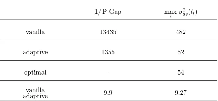
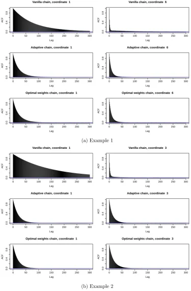
Example 1. In case where the correlation matrix of the target distribution has blocks of highly correlated coordinates, one would prefer to update them more fre-quently than the others. In this section we construct an artificial example where the upper bound in (2.12) is d₂Gap 1_d. Consider a target distribution inRd,d= 2k with correlation and normalised precision (inverse covariance) matrices given re-spectively by their block form, i.e., Corr = (Cij)k_i,j₌₁,Q= (Qij)k_i,j₌₁, where Cij and Qij are 2×2 matrices such that all Qij, Cij are zero matrices if i 6=j and for all

i= 1, . . . , k

Cii=      

1 −ρi

−ρi 1

     

, Qii=

     

1 ρi

ρi 1

(37)

where we assume ρi ≥0,i= 1, . . . , k. Assume one wants to apply the

coordinate-wise RSGS to sample from a distribution with the above correlation matrix.

Proposition 1. Let the inverse covariance matrix Q be as above. Define

αi =

Qk

l=1,l6=i(1−ρl)

Pk

l=1

Qk

j=1,j6=l(1−ρj)

. (2.13)

Then the pseudo-optimal weights are given by

popt₂_i₋₁ =popt₂_i = αi

2. (2.14)

The correspondingP-Gap is

P-Gap popt=

Qk

l=1(1−ρl)

2Pk

l=1

Qk

j=1,j6=l(1−ρj)

. (2.15)

Without loss of generality assumeρ1 = max{ρ1, . . . , ρk}. We shall compare

pseudo-spectral gaps of the vanilla chain with RSGS(popt). One can easily obtain that the pseudo-spectral gap of the vanilla chain is given by

P-Gap 1 d = 1

d(1−ρ1).

Simple calculations yield

lim

ρ1→1

P-Gap _d1

P-Gap (popt₎ = lim_ρ

1→1

1−ρ1

2k

_Q_k

l=1(1−ρl)

2Pk l=1

Qk

j=1,j6=l(1−ρj)

= lim

ρ1→1

1 k Pk l=1 Qk

j=1,j6=l(1−ρj)

Qk

l=2(1−ρl)

= 1 k = 2 d. Moreover, lim

ρ1→1

max i dp opt i = 1 k = 2 d.

Thus, we obtained a sequence of precision matrices for which the pseudo-optimal weights improve the pseudo-spectral gap by d₂ times in the limit which is the upper bound in (2.12). Notice, if the underlying target distribution is normal, the upper bound in (2.11) for theL2−spectral gap is approximated.

(38)

RSGS (i.e., with the uniform selection probabilities). Moreover, from Corollary 2 to Theorem 5 ofRoberts and Sahu [1997a], lim

ρ1→1

Gap(DUGS)

P-Gap(1 d)

= 2. We constructed an

example of a 3-diagonal precision matrix, where in dimensions greater than 6, RSGS with pseudo-optimal weightspopt converges d₄ times faster than DUGS for ρ1 →1.

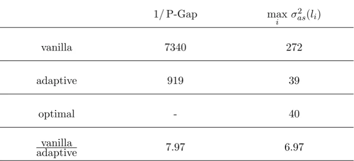
Example 2. One mistakenly might conclude that significant gain from using the pseudo-optimal weights is achieved only if some of the off-diagonal entries of the covariance matrix are close to one . Here we provide a somewhat counter-intuitive example that demonstrates fallacy of such statement.

Consider a correlation matrix matrix given by Σ(2) = (Cij)d_i,j₌₁, whereCii= 1 fori= 1, . . . , d,C1i=Ci1:=ci ≥0 for i= 2, . . . , dand all other entries Cij = 0.

One can easily work out that the smallest eigenvalue of Σ(2), λmin = 1−

q Pd

i=2c2i. Thus, if λmin >0, then Σ(2) is a valid correlation matrix. Set d = 50

andci = ₇_.1₀₁ ≈0.143 fori= 2, . . . ,50.

We run the subgradient optimisation algorithm presented in Section 2.4 in order to estimatepopt. We estimatepopt₁ ≈0.484,popt_i ≈0.01 fori= 2, . . . ,50. From (2.9) the pseudo-spectral gap is roughly ₁₄₉₆1 , whilst P-Gap ₅₀1 is roughly ₁₈₂₉₄1 . Thus, if the target distribution is normal, the spectral-gap of the vanilla RSGS is improved by more than 12 times. Note, however, all off-diagonal correlations are less than 0.143.

2.4 Adapting Gibbs Sampler

In this section we derive the Adaptive Random Scan Gibbs Sampler (ARSGS) Al-gorithm9. We provide all the steps and intuition leading towards the final working version of the algorithm presented in the end of the section.

The goal is to compute the pseudo-optimal weights (2.10) for the RSGS (2.1). However, in practice the correlation matrix of the target distribution is usually not known. Thus, we could proceed in the adaptive way, similarly to Haario et al. Haario et al.[2001]. Given output of the chain of length n, let Σb_n,Qnb , andD[(p)_n be estimators of Σ,Q, andDprespectively built upon the chain output. For instance,

one may choose the naive estimator

b Σn=

1

n n

X

i=0

XiX_iT−(n+ 1)XnXT_n

!

, (2.16)

(39)

to timen.

Algorithm 5:Adaptive Random Scan Gibbs Sampler (general idea) Generate a starting locationX0 ∈Rd. Set an initial value of p0∈∆s−1.

Choose a sequence of positive integers (km)∞m=0. Setn= 0,i= 0.

1. n:=n+ki. Run RSGS(pi) for ki steps;

2. Re-estimateΣb_n andD\(pi)_n;

3. Computepi+1 = argmax_p∈∆s−1λmin

\

D(pi₎

nQnb

;

4. i:=i+ 1.

The Algorithm 5 summarises the above ideas. The algorithm is limited by Step3, where one needs to maximise the minimum eigenvalue. Maximising the min-imum eigenvalue is known to be a complicated optimisation problem. There is vast literature covering optimisation problem in Step 3 and we refer to Overton [1988, 1992], Chu [1990], and references therein. Unfortunately, the existing optimisation algorithms require computation of the minimum eigenvalues of λmin

[

D(p)_nQnb

, which is an expensive procedure. Since at every iteration of Algorithm5the weights

pi are subotimal, it is reasonable to solve the optimisation problem in Step 3 ap-proximately in order to reduce the computational time of each iteration. Therefore, we develop a new algorithm based on the subgradient method for convex functions (see Chapter 8 ofBertsekas [2003]) applied to (2.10).

Forε >0, introduce a contraction set of ∆s:

∆ε_s:={w∈_Rs|wi ≥ε, i= 1, . . . , s−1; 1−w1− · · · −ws≥ε}, (2.17)

and consider (d+ 1)×(d+ 1) matrices

Qext = diag (Q,1),

Σext_n = diagΣb_n,1

,

Dext_w = diag Dw, 1− s

X

i=1

wi

!

,

Σext= diag (Σ,1),

Qext_n = diagQb_n.1

,

D_next(w) = diag D\(w)_n, 1−

s

X

i=1

wi

!

(40)

Let us denote the target function

f(w) =λmin DwextQext

=λmin

p

Qext_Dext w

p

Qext_, _(2.18)

where the last equality holds in view of Lemma2.

Using the definition of the pseudo-optimal selection probabilities (2.10), one can easily verify the following proposition

Proposition 2. The pseudo-optimal weights (2.10) can be obtained as a normalised solution of

w? = argmax

w∈∆s

f(w),

i.e.,

popt_j = w

? j

w₁?+· · ·+w?

s

, j= 1, . . . , s, (2.19)

Moreover,

P-Gap(popt) = 1

(w?₁+· · ·+w?

s)

f(w?),

where f is defined in (2.18).

Remark. One could easily avoid introducing the extended matrices Σext, Qext by simply settingps= 1−p1− · · · −ps−1 and treating function λmin

[

D(p)_nQb_n

as a function ofs−1 variables. However, we found empirically, that such approach can significantly slow down convergence of the ARSGS Algorithm9 introduced later in this section.

It is easy to prove concavity of the function f (2.18).

Proposition 3. Function f defined in (2.18) is concave in∆s.

Andrew et al. [1993] show that f is differentiable at w ∈ ∆s if and only

if f(w) is a simple eigenvalue of pQext_Dext w

p

Qext_{. It is also known that convex}

functions in Euclidean spaces are differentiable almost everywhere w.r.t. Lebesgue measure (seeBorwein and Vanderwerff[2010], Section 2.5). Andrew et al.[1993] also provide exact formulas for computing derivatives of f where they exist. Thus, we are motivated to adapt subgradient method for convex functions in order to modify Step 3 in the above algorithm.

(41)

Definition. Let h:Rd →R be a convex function. We say v is a subgradient of h at point x if for ally∈Rd,

h(y)≥h(x) +hy−x, vi.

If h is concave, we say that v is a supergradient of h at a point x, if (−v) is a subgradient of the convex function(−h)atx. The set of allsub−(super−)gradients

at the point x is called sub-(super-)differential at x and is denoted by∂h(x).

In other word,∂h(x) parametrises a collection of all tangent hyperplanes at a pointx.

Note thatf(w) = 0 on the boundary of ∆s. Therefore, the maximum off is

attained inside ∆s. One may apply the subgradient optimisation method in order

to estimatepopt. The method is described in Algorithm 6.

Algorithm 6:Subgradient optimisation algorithm

Set an initial value ofw0 = (w0₁, . . . , w_s0)∈∆s. Define a sequence of

non-negative numbers (am)∞m=1 such that

P∞

m=1am =∞ and

limm→∞am = 0. Seti= 0.

1. Compute anydi∈∂f(wi). Normalisedi:= _|_di di 1|+···+|dis|; 2. w_jnew:=wi_j+ai+1dij,j= 1, . . . , s;

3. wi+1 := Pr∆s(w

new_{) , where Pr}

∆s is the projection operator on ∆s;

4. i:=i+ 1.

It is known that Algorithm 6 produces a sequence{wi} such that wi →w?

asi→ ∞(see Chapter 8 ofBertsekas[2003]). Therefore, it is reasonable to combine the Algorithm5with the subgradient algorithm. In order to do so, define a sequence of approximations of (2.18):

fn(w) =λmin Dextn (w)Qextn

=λmin

p

Qext

n Dnext(w)

p

Qext n

.

(42)

Algorithm 7: Adaptive Gibbs Sampler based on subgradient optimisa-tion method (not implementable)

Generate a starting locationX0 ∈Rd. Fix s+11 > ε >0. Set an initial

value of w0 = (w0₁, . . . , w_s0)∈∆ε_s. Define a sequence of non-negative numbers (am)∞m=1 such that

P∞

m=1am =∞ and limm→∞am = 0 . Set i= 0. Choose a sequence of positive integers (km)∞m=0.

Beginning of the loop 1. n:=n+ki. pij :=

wi

j

wi

1+···+wis,j = 1, . . . , s. Run RSGS(p

i_{) for} _k i steps;

2. Re-estimateΣb_n andDext_n (w);

3.1. Computedi ∈∂fn(wi). Normalisedi := _|_di di 1|+···+|dis|; 3.2. w_jnew:=wi_j+ai+1dij,j= 1, . . . , s;

3.3. wi+1 := Pr∆ε s(w

new_{) , where Pr} ∆ε

s is the projection operator on ∆

ε

s;

4. i:=i+ 1.

selection probabilities that are on the boundary of ∆s−1 is not ergodic. Secondly,

this assumption is motivated by the results of Latuszy´nski et al. [2013b], where it is a minimum requirement to establish convergence of an Adaptive Gibbs Sampler. Finally, in the final Algorithm9, it is an essential assumption to be able to perform power iteration Step 3.1.1. Note, however, that ε > 0 may be chosen arbitrary small.

In order to construct an implementable and practical ARSGS algorithm, we still need to find a way to approximate the subgradient∂fn(wi) in Step3.1and also

find a cheap way of computing the projection Pr∆ε s(w

new_{) in Step} _3.3_.

An efficient algorithm to compute the projection on ∆ε_sis presented inWang and Carreira-Perpi˜n´an [2013] and summarised in Algorithm 8. First, we increase all small coordinates to be ε in Step 1. If the resulting point is outside ∆ε_s, we need to project it on the hyperplane {w ∈ Rs|1−Psj=1wj = ε, wi ≥ ε}. In

order to find the projection, we first rescale the coordinates in Step3. Then we use the algorithm ofWang and Carreira-Perpi˜n´an [2013] to compute the projection on

{w∈Rs|Psj=1w= 1, wi ≥0}in Steps4- 6. Finally, we rescale the resulting point

in Step7 and thus, obtain the desired projection.

(43)

Algorithm 8:Projection on ∆ε_s

The output of the algorithm iswproj - projection ofw∈_Rs _{onto ∆}ε

s.

1. Define an auxiliary variable waux:=w. Forj = 1, . . . , s, ifwaux_j < ε, set

waux

j :=ε;

2. If 1−Ps

j=1wauxj > ε, then wproj:=waux and go to Step 8;

else go to Step3;

3. Forj= 1, . . . , s,w_jtemp:= ₁₋_ε₍1_s₊₁₎(waux_j −ε);

4. Sort vector (w₁temp, . . . , wtemps ) intou: u1 ≥ · · · ≥us;

5. ρ:= max (

1≤j≤s: uj +1_j

1−Pj

k=1uk

>0 )

;

6. Defineλ= 1_ρ 1−Pρ

k=1uk

;

7. Forj= 1, . . . , s,w_jproj:=ε+ (1−ε(s+ 1)) max{wtemp_j +λ,0};

8. Returnwproj.

∂fn(wi) in Step 3.1 of Algorithm 7. Since fn(w) is the minimum eigenvalue of a self-adjoint matrix, fn(w) may be obtained as

fn(w) = min

x:kxk=1

Dp

Qext

n Dnext(w)

p

Qext

n x, x

E

,

wherex∈Rd+1 and h·,·idenotes scalar product in Rd. Define

g_xn(w) =DpQext

n Dextn (w)

p

Qext

n x, x

E

.

Let∇denote a gradient w.r.t. w. Then

∇gnx(w) =

p

Qext n

∂Dextn (w)

∂w1

p

Qext n x, x

, . . . , p Qext n

∂Dnext(w)

∂ws

p

Qext n x, x

. (2.20)

Here _∂w∂

(44)

∂fn(w) = conv

(

∇gx(w)

x: pQext

n Dextn (w)

p

Qext

n x=fn(w)x, kxk= 1

)

,

where conv{A} denotes a convex hull of the setA.

Computing elements of the set ∂fn(w) is computationally expensive, since one has to calculate the minimum eigenvectors ofpQext

n Dextn (w)

p

Qext

n . Therefore,

we look for a cheap approximation of the points∇g_xn(w) in ∂fn(w).

Let y =pQext

n x. Since we are interested in minimum eigenvectors x, such

that

p

Qext

n Dnext(w)

p

Qext

n x=fn(w)x,

we can rewrite this equation as

1

fn(w)

y= Dext_n (w)−1Σext_n y. (2.21)

That is, computing the minimum eigenvector of pQext

n Dnext(w)

p

Qext

n is

equivalent to computing the maximum eigenvector of Dext_n (w)−1Σb_n. Given y that solves (2.21) and substituting x= 1

k√Σext

n yk p

Σext

n y into (2.20), we obtain

∇gn_x(w) = 1

kp

Σext

n yk2

D∂Dext

n (w)

∂w1 y, y

E

, . . . ,

D∂Dext

n (w)

∂ws y, y

E !

. (2.22)

We can do further transformations. Let

D_next(w)−1=Ln(w)LT_n(w) (2.23)

be the Cholesky decomposition of Dext_n (w)−1

, where Ln(w) is a lower

tri-angular matrix. Definez:=L−_n1(w)y and

Ri(w) := diag

0, . . . ,0, 1

wi

, . . . , 1

wi

,0, . . . ,0,− 1

1−w1− · · · −ws

, (2.24)

where _w1

i are placed exactly on the positions of the diagonal elements of Qii in the partition Q = (Qij)s_i,j₌₁. Then after simple manipulations, (2.21) and (2.22) are

equivalent respectively to

LT_n(w)Σext_n Ln(w)z= 1

(45)

and

∇gn_x(w) = 1

hLT

n(w)Σextn Ln(w)z, zi

hR1(p)z, zi, . . . ,hRs−1(p)z, zi

!

, (2.25)

where we used the block-diagonal structure ofLn(w) and a representation

∂Dext_n (w)

∂wi

= diag 0, . . . ,0, Q−_ii1,0, . . . ,0,−1

.

Because of the normalisation in Step 3.1 of the Adaptive Gibbs Sampler 7, (2.22) and (2.25) imply that a supergradient of fn(w) is proportional to

dy(w) = (Dext_n (w))1y, y

, . . . ,(Dext_n (w))s−1y, y

, (2.26)

or, in terms of z, to

dz(w) = (hR1z, zi, . . . ,hRsz, zi), (2.27)

wherey and z are the maximum eigenvectors of Dext_n (w)−1 b Σn and

LT_n(w)Σext_n Ln(w), respectively. Here the lower triangular matrix Ln(w) is defined

by the Cholesky decomposition (2.23).

Power iteration step may be performed in order to approximate y and z. Let z0 and y0 be randomly generated unit vectors. Then at every iteration of the

algorithm, we compute

yi+1=Qextn Dnext(wi)yi, (2.28)

zi+1 =LTn(wi)Σextn Ln(wi)zi. (2.29)

and use the normalised vectors yi+1 and zi+1 instead of y and z when computing

the directions (2.26) and (2.27)

Given the intuition above, we present two versions of the ARSGS in the Algo-rithm9, where in round brackets we denote an alternative version of the algorithm. One might notice the perturbation termbi+1ξi+1 in the Step 3.1.1. In fact,

without the perturbation we may break the algorithm due to the fact that the power iteration step may fail to approach the maximum eigenvalue. It happens when zi

(oryi) ”slips” into the eigenspace of a wrong eigenvalue and can’t get out of it for the subsequent algorithm steps.