Band structure interpolation using optimized local orbitals
from linear-scaling density functional theory
L. E. Ratcliff,1G. J. Conduit,2N. D. M. Hine,1,3,4and P. D. Haynes1,3,2,*
1Department of Materials, Imperial College London, Exhibition Road, London SW7 2AZ, United Kingdom
2Theory of Condensed Matter, Cavendish Laboratory, University of Cambridge, J. J. Thomson Avenue, Cambridge CB3 0HE, United Kingdom 3Department of Physics, Imperial College London, Exhibition Road, London SW7 2AZ, United Kingdom
4Department of Physics, University of Warwick, Coventry CV4 7AL, United Kingdom
(Received 28 March 2018; revised manuscript received 27 June 2018; published 11 September 2018)
Several approaches to linear-scaling density functional theory (LS-DFT) that seek to achieve accuracy equivalent to plane-wave methods do so by optimizingin situa set of local orbitals in terms of which the density matrix can be accurately expressed. These local orbitals, which can also accurately represent the canonical Kohn-Sham orbitals, qualitatively resemble the maximally localized Wannier functions employed in band structure interpolation. As LS-DFT methods are increasingly being used in real-world applications demanding accurate band structures, it is natural to question the extent to which these optimized local orbitals can provide sufficient accuracy. In this paper, we present and compare, in principle and in practice, two methods for obtaining band structures. We apply these to a (10, 0) carbon nanotube as an example. By comparing with the results from a traditional plane-wave pseudopotential calculation, the optimized local orbitals are found to provide an excellent description of the occupied bands and some low-lying unoccupied bands, with consistent agreement across the Brillouin zone. However free-electron-like states derived from weakly bound states independent of theσ andπ
orbitals can only be found if additional local orbitals are included.
DOI:10.1103/PhysRevB.98.125123
I. INTRODUCTION
Methods for inferring detailed information about the elec-tronic structure throughout the first Brillouin zone (BZ) from first-principles calculations on a discrete mesh of Bloch wave vectors [1–4] have received significant attention over the last 15 years. The most popular approach to date has been the interpolative scheme based upon maximally localized Wan-nier functions (MLWFs) [2,5,6] obtained by a post-processing of the results from standard codes [7,8]. These methods have been used for a wide range of applications, not just within density functional theory (DFT) but also many-body perturbation theory within both the GW approximation [9] and Bethe-Salpeter equation [10] due to their importance for theoretical spectroscopy. Other notable applications include electric polarization [11–13], orbital magnetization [14–16], and topological insulators [17–19]. These and others have been described in a recent review alongside the theory of Wannier functions [6].
Linear-scaling orO(N) methods for first-principles elec-tronic structure calculations [20–22] based on DFT now pro-vide routine access to the total energy and atomic forces [23] of systems consisting of many thousands of atoms [24,25], giving rise to new opportunities for applications in different fields, as discussed, for example, in recent reviews on the subject [26,27]. Methods that optimize a set of Wannier-like localized orbitals [28–32] are also capable of achieving accu-racy equivalent to plane waves (PWs) or other systematic basis
sets [31,33]. This paper explores the use and limitations ofin situoptimized orbitals, often referred to as support functions, for band structure interpolation.
Due to the large simulation cells appropriate for linear-scaling methods, the correspondingly small BZs are sampled using the-point only, with the added benefit that the local orbitals may be chosen to be real rather than complex. How-ever, in the contemporary DFT approach, the total energies and atomic forces computed represent averages of the valence electronic structure across the BZ and return relatively little information about the system in view of the effort invested in their calculation. Moreover, the support functions are formally related [34] to the canonical Kohn-Sham (KS) orbitals and therefore, in principle at least, contain far more information about the electronic structure.
It is straightforward to obtain the KS energies and orbitals from the support functions by a single diagonalization of the ground-state self-consistent KS Hamiltonian matrix. Al-though such a postprocessing step does not scale linearly, the minimal size of the local orbital set means that its contribution to the overall computational cost remains small for systems containing up to several thousand atoms. A method for per-forming band structure interpolation across the BZ based upon the local orbitals would therefore provide much richer information about the electronic structure, allow a detailed assessment of the accuracy of this description, and provide a basis for further calculations, including (local) densities of states (DOS).
cost prohibits the standard approach of extracting MLWFs from cubic-scaling DFT. The use of a support-function-based approach would therefore be invaluable for applications such as generating band structures of materials containing low defect concentrations and calculating quantities such as ef-fective masses. Where applicable, supercell band structures can then be compared to those obtained from primitive cell calculations, using unfolding or projection techniques. As an example, a spectral function projection method which uses such localized orbitals to obtain bandstructures for the primitive cell [35], has been used to obtain insights into the behavior of various complex heterostructures compared with the equivalent monolayers [36,37].
Despite the formal connection between support functions and MLWFs, the extent to which they form an accurate basis for band structure interpolation in practice has not previously been explored. In other words, do the approximations made in a typical calculation, such as the imposition of strict local-ization radii or imperfect convergence, prevent accurate band structure interpolation? In this paper, we answer this question, while also considering what is the best method for obtaining band structures from a support function basis.
Methods for calculating band structures fall into two main classes, each relating to one of the two equivalent statements of Bloch’s theorem. Codes based upon atomic-type basis sets adopt the interpolative tight-binding (TB) approach that is also employed for Wannier interpolation [2,5], whereas within PW codes, an extrapolative approach [3] based onk·p
perturbation theory [38] has been successfully implemented [39]. To compare the two methods, we choose to use the basis of localized orbitals generated by the linear-scaling method implemented in the ONETEP code [34,40]; however, similar results would be expected for related methods. In principle, the localized orbitals of ONETEP, referred to as nonorthog-onal generalized Wannier functions (NGWFs) [32], straddle both approaches: they form a minimal basis of local orbitals that have been optimized in terms of an underlying basis equivalent to a set of PWs. When implemented within the ONETEP code, the two approaches give similar but different results that are interpreted here in terms of a simple one-dimensional Kronig Penney model.
The paper is organized as follows: in Sec.II, the relevant theory underlying the ONETEP method is outlined, and two approaches are described by which the KS energies and or-bitals may be obtained at a general point in the BZ. In Sec.III, these two methods are compared for a one-dimensional toy model that illustrates the advantages and disadvantages of each. Section IV discusses the results obtained from both approaches when implemented in the ONETEP code and applied to a carbon nanotube (CNT). Conclusions are drawn in Sec.V.
II. METHODOLOGY
A. Linear-scaling methods
The single-particle density matrix (DM)ρ(r,r) provides a complete description of the fictitious KS system in DFT. The DM may be described in the diagonal representation provided by the canonical KS orbitals{ψn(r)}and associated
occupancies {fn} (where fn=1 for occupied states lying below the chemical potential andfn=0 otherwise) or more generally in terms of a set of nonorthogonal orbitals{φα(r)} and a so-called density kernelKαβ:
ρ(r,r)= n
ψn(r)fnψn(r)=
αβ
φα(r)Kαβφβ(r). (1)
Note that spin and k-point labels have been dropped, the former for simplicity and the latter due to the assumption of -point sampling justified above. Equation1 takes the form of a similarity transformation where there is a linear transfor-mation between the canonical and nonorthogonal orbitals. For a linear-scaling method, it is necessary to choose a represen-tation in which the nonorthogonal orbitals are also localized in space and to exploit the nearsightedness of the DM [41] by enforcing sparsity on the density kernel. The ground state of a system may then be found by minimizing the total energy with respect to the DM subject to the constraints of normalization and idempotency [42–45].
In ONETEP, the minimization is performed both with respect to the density kernel [46] and the NGWFs [32]. Various methods exist to calculate the density kernel at linear scaling cost; in ONETEP a combination of purification [42] and penalty functional [47] approaches are used, as described in detail elsewhere [46]. The initial guess for the NGWFs consists of a set of fireballs (FBs) [48], which are generated by self-consistently solving the KS equations for an isolated atom using the same pseudopotential and exchange correla-tion funccorrela-tional as for the full system. The NGWF optimizacorrela-tion is then carried out by expanding them in terms of a basis set of primitive functions that have been variously known as periodic cardinal sine (psinc) [49], Dirichlet [50], or Fourier Lagrange [51] functions. These functions are the discrete equivalent of the Dirac delta function, which are arranged on the grid points of a regular mesh commensurate with the simulation cell. Each NGWF is associated with an atom and is expanded in a restricted set of psinc functions whose grid points lie within spheres of a given radius centered on that atom. Fast Fourier transforms (FFTs) may then be employed as in PW codes to apply the Hamiltonian; in particular, the kinetic energy [52], with a reduced FFT box [53] used consistently to achieve linear scaling.
ONETEP has been shown to achieve linear scaling for the entire calculation with controlled accuracy comparable to that of PW pseudopotential codes [54]. The result is a set of NGWFs, each of which has been optimizedin situaccording to its individual chemical environment in terms of a basis equivalent to a set of PWs. A minimal set of NGWFs may then be used successfully whilst avoiding some of the pitfalls of local orbitals such as basis set superposition error [55].
overestimated, with some states not captured at all [54,56]. To overcome this problem, a method has been devised wherein a second set of NGWFs are optimized to explicitly represent a select number of (bound) conduction states. The density operator, ˆρ, is used to project out the valence states, so when a sufficiently large energy shiftσ is applied, the conduction states of interest become lower in energy than the valence states. The Hamiltonian operator therefore becomes
ˆ
H →Hˆ −ρˆ( ˆH−σ) ˆρ. (2)
Using this Hamiltonian, a second non-self-consistent calcu-lation can be performed following a ground state calcucalcu-lation to obtain a set of conduction NGWFs and associated density kernel, for which the total occupancy corresponds to the requested number of conduction states. To reach a comparable level of accuracy, the conduction NGWF radii are typically larger than those required for valence NGWFs. Before diago-nalizing the unprojected Hamiltonian, the conduction NGWFs are combined with the valence NGWFs to form a joint basis. Provided sufficiently large localization radii are used, the joint basis is capable of representing both the occupied and unoc-cupied KS states to a similar high level of accuracy [56,57].
B. Band structure calculation
For any periodic system that is invariant under translation by a lattice vectorR, Bloch’s theorem states that any eigen-state of the Hamiltonianψ(r) must satisfy
ψ(r+R)=eik·Rψ(r), (3)
wherekis the Bloch wave vector or crystal momentum. An equivalent statement is
ψ(r)=eik·ru(r), (4)
whereu(r)=u(r+R) is a cell-periodic function. IfGis a reciprocal lattice vector such thateiG·R=1, then from the first formulation Eq. (3) it is clear that the statements of Bloch’s theorem for wave vectorskandk+Gare identical and these may be considered equivalent. Hencekmay be chosen from the first BZ and the band structure may be represented as periodic in reciprocal space.
The KS Hamiltonian takes the following general form (in Hartree atomic units ¯h=me=1):
ˆ
H = −1
2∇
2+V(r)+
I
|pIEIpI|, (5)
where the local potentialV(r) is cell-periodic and the third term represents the action of a nonlocal norm-conserving pseudopotential in separable form [58] in which I is a composite index running over ions and angular momentum channels,{|pI}are the projectors, and {EI}the associated energies.
To calculate the band structure from a linear-scaling calcu-lation, it is necessary to obtain the KS energies and orbitals at an arbitraryk-point in terms of a set of real local orbitals, e.g., NGWFs optimized in a self-consistent ground-state total energy calculation using the-point only.
1. NGWF approach
We now present two approaches to calculating the band structure, one of which is inspired by Eq. (3) and related to TB and Wannier interpolation, in which the wave function at a generalk-point with band indexnis written
ψnTBk(r)= R
eik·R
α
cTBnkαφα(r−R), (6)
involving a sum over all lattice vectors R. In this approach, identical copies of each NGWF for each cell are made from the home cell (R=0). The Hamiltonian for a generalk-point is then constructed from Eq. (5) with additionalk-dependent phase factors arising when a matrix element corresponds to NGWFs from neighboring cells. This is straightforward when the NGWFs are localized within a single cell—the
k-dependent Hamiltonian matrix elements are written as
HαβTB(k)= φα|Hˆ|φβ
i
θ(ki, rαi−rβi, Ri), (7)
where rα(β) is the center of φα(β) expressed in fractional coordinates, and the one-dimensional phase factorsθtake the form
θ(k, r, R)= ⎧ ⎪ ⎨ ⎪ ⎩
1 |r| 12 eikR r > 1
2
e−ikR r <−1 2
. (8)
Diagonalization of this Hamiltonian yields the KS energies and orbitals, i.e., the set of expansion coefficients{cTB
nkα}, for the wave vectork.
An alternative approach relates to the second formulation of Bloch’s theorem Eq. (4), which expresses the wave function as
ψnKPk(r)=eik·runk(r)=eik·r
α
cKPnkα R
φα(r−R), (9)
where the expansion of unk(r) in terms of NGWFs is ex-plicitly cell-periodic, a construction that fits naturally with a PW or psinc basis set. Indeed, this approach is success-fully employed in PW calculations. As suggested by k·p
perturbation theory, the Bloch phase factor may be treated analytically to derive ak-dependent Hamiltonian that acts on the cell-periodic part of the wave function
ˆ
H(k)= −1 2∇
2−ik· ∇ +k2
2 +V(r)
+
I
|pI(k)EIpI(k)|, (10)
where the phase factor has been incorporated into the pro-jectors, which have thus become k-dependent: r|pI(k) =
eik·rp
I(r). In contrast to Eq. (7), the Hamiltonian matrix elements do not contain any additional phase factors and are simply calculated as
HαβKP(k)= φα|Hˆ(k)|φβ. (11)
As for the TB method, the k·p band structure is again obtained by diagonalization.
III. TOY MODEL
Before comparing the two approaches to calculating band structures using ONETEP, we first make use of a simple one-dimensional model. In the following, we describe the setup of this toy model, i.e., the choice of potential and definition of the localized basis sets which are designed to mimic some of the features of ONETEP NGWFs. Using this model, we identify characteristic features of the two methods for cases where the basis set is incomplete using both analytic and numerical analyses.
A. Description of the Model
We choose to use the one-dimensional Kronig-Penney model, where the Hamiltonian is defined as
ˆ
H = −1
2
d2
dx2 +V(x), (12)
with a periodic potentialV(x)=V(x+L), given by
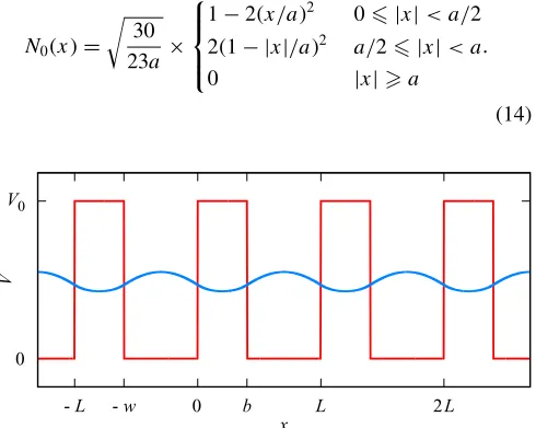
V(x)=
V0 0x < b
0 −wx <0, (13)
and the lattice parameterL=b+w. The potential and lowest energy state are illustrated in Fig.1.
The band structure for this model may be found by solving a transcendental equation numerically. This is used as a refer-ence for results obtained from a fully numerical approach em-ploying piecewise polynomial nonorthogonal basis functions (to mimic the role of NGWFs of different quality) for which Hamiltonian matrix elements may be found analytically. Basis functions are centered on the nodes of a regular grid with spacingasuch thatL=Ma.
The first basis is piecewise quadratic and continuous up to and including the first derivative. Basis functions only overlap their nearest neighbors. The function centered at x=0 is denotedN0(x) and thenNm(x)≡N0(x−ma) is centered at
x=ma.
N0(x)= 30 23a ×
⎧ ⎪ ⎨ ⎪ ⎩
1−2(x/a)2 0|x|< a/2 2(1− |x|/a)2 a/2|x|< a
0 |x|a
.
(14)
0 V0
-L -w 0 b L 2L
V
[image:4.590.313.546.104.187.2]x
FIG. 1. Potential (red) for the Kronig Penney model with the lowest energy state (blue) (atk=0) superimposed.
The second basis consists of cubic B-splines [28] continu-ous up to the second derivative but twice as wide as the first set and hence overlapping up to third-nearest neighbors.
B0(x)
= 140 151a ×
⎧ ⎪ ⎪ ⎪ ⎨ ⎪ ⎪ ⎪ ⎩
1 − (3/2)(x/a)2
+ (3/4)(|x|/a)3 0|x|< a (1/4)(2− |x|/a)3 a |x|<2a
0 |x|2a
.
(15)
These two functions have been chosen to examine the effect of basis set quality. In particular, the optimization process for NGWFs imposes no explicit constraints on their continuity, either at the boundary or inside the localization region. Instead, continuity is desirable because it minimizes the kinetic energy, since the Fourier transform ˜f(q) of a function f(x) decays as q−(n+1), where n is the order of lowest discontinuous derivative. Hence the behaviours of the
N andBbases are expected to differ qualitatively.
B. Free-electron limit
First, the free-electron V0=0 limit is examined. In this case, the exact forms of the wave functions are known:
ψnk(x)∼ei(k+nG)x where G=2π/L. The discrete transla-tional symmetry (invariant under translation by any multiple of a) of the Hamiltonian constructed using the N and B
bases can similarly be exploited to write down the eigenvec-tors cTB
nkm=e2π i(k/G+n)m/M/ √
M and cKP
nkm=e2π inm/M/ √
M
where the index mlabeling the center of the basis function is analogous to the NGWF indexαin Eqs. (6) and (9).
In the free-electron limit, the translational invariance also means that matrix elements depend only on the separation of the basis centres, i.e., for some operator ˆO, the matrix elements for theBbasis between functions centered atx=la
andx=ma,Olm=om−l, where
on=
B0(x) ˆO Bn(x)dx. (16)
Matrix elements for the overlap ˆO≡1, momentum ˆO≡
−id/dx and kinetic ˆO≡ −(1/2)d2/dx2 operators are sum-marized in TableI. In this special case, band structures may be calculated analytically from the expectation values of the TB andk·pHamiltonians in the corresponding eigenstates.
TABLE I. Overlap, momentum, and kinetic energy matrix ele-ments for the two basis sets employed in Sec.IIInormalized such that s0=1. By symmetry p0=0 ando−n=o∗n, whereomay be
replaced bys,p, ort. Results for each basis should all be divided by the number shown in the second (÷) column.
Overlap Momentum Kinetic
÷ s1 s2 s3 ip1a ip2a ip3a t0a2 t1a2 t2a2 t3a2
N 46 7 0 0 30 0 0 80 −40 0 0
[image:4.590.41.286.516.712.2]Defining θnk=2π(k/G+n)/M, the band structure for the TB approach (including overlaps up to third-nearest neighbor) is given by
εnTB(k)= t0+2t1cosθnk+2t2cos 2θnk+2t3cos 3θnk
s0+2s1cosθnk+2s2cos 2θnk+2s3cos 3θnk
,
(17)
which is a quotient of Fourier series as expected from TB. This is manifestly periodic in reciprocal space, i.e.,εTB
n (k)=
εnTB(k+G). Similarly,
εKPn (k)= 1 2k
2+Tn+Pn|k|
Sn
, (18)
where for basis functions that overlap up to third-nearest neighbors,
Sn=s0+2s1cosθn0+2s2cos 2θn0+2s3cos 3θn0, (19)
and similarly forTnin terms of{tm}. ForPn,
Pn=2(−1)ni[p1sinθn0+p2sin 2θn0+p3sin 3θn0]. (20)
This takes the form of an expansion aboutk=0 and is not pe-riodic ink, so that degeneracy of bands at the BZ boundary is not guaranteed. However, this method does return the correct effective mass for all bandsn:mKP
n (k)=(d2εn/dk2)−1=1. By contrast, expanding the TB result for the lowest band (n=0) aboutk=0,εTB
0 (k)≈T0/S0+k2/[2mTBn (0)], where
mTBn (0)= S
2 0/2
(s1+4s2+9s3)T0−(t1+4t2+9t3)S0. (21)
For theN basis,mTB
n (k=0)=3/4 whereas for theBbasis the correct value is obtained. Hence the accuracy of the band curvature depends upon the quality of the basis used.
Both methods predict the same value for the bottom of the lowest bandε0(0)=T0/S0 which should vanish. This is the case for both bases used here, but is not a universal feature and depends upon the ability of a basis set to describe exactly the lowest stateψ00(x)=1/√L, i.e., a constant.
The qualitative difference between the two basis sets is clearly demonstrated by examiningε1(0). For both methods, the B basis is correct to leading order with an error of orderM−6 whereas theN basis is wrong by a factor of 4/3 consistent with the error in the TB effective mass.
The methods are also distinguished by examining the ener-gies of the lowest two bands at the BZ boundary, which should be degenerate. The TB method guarantees this by construc-tion, but for thek·pmethod this is not the case, so that for a poor quality basis gaps appear at the BZ boundary. Indeed, for the k·p method, for k→k+G,uk+G(x)=uk(x)eiGx and thus the basis used to describeuk(x) must also be able to describe its product witheiGx. For all but a few high energy PWs at the edge of the cutoff sphere, this product is perfectly represented in a PW basis and so no such gaps arise. However for the toy model, and as will be seen in the following also for the NGWF basis, this is not expected to be the case.
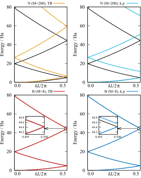
To illustrate this point, we have considered two types of poor quality basis set: an intrinsically lower quality basis which is nonetheless well converged in terms of the number of basis functions, i.e., basisN withM=200, and a basis
0 20 40 60 80
0.0 0.5
Energy / Ha
kL/2π
N (M=200), k.p
0 20 40 60 80
0.0 0.5
Energy / Ha
kL/2π
N (M=200), TB
0 20 40 60 80
0.0 0.5
Energy / Ha
kL/2π
B (M=8), k.p
0 20 40 60 80
0.0 0.5
Energy / Ha
kL/2π
B (M=8), TB
44.2 44.4 44.6 44.8
0.495 0.500 44.2
44.4 44.6 44.8
[image:5.590.308.552.60.369.2]0.495 0.500
FIG. 2. Low energy free-electron band structures for theN(top) andB(bottom) basis sets using both the TB (left) andk·p(right) methods. The analytical solution is shown for reference (black lines).
set which is of high quality but with an insufficient number of basis functions, i.e., basis B with M=8. In terms of ONETEP, these two setups might loosely be compared to a set of NGWFs with large enough localization radii but which have been poorly optimized (e.g., loose convergence thresholds) or not optimized at all, and to NGWFs which have been well optimized but which have insufficient degrees of freedom, e.g., due to localization radii which are too small.
Using these two setups, we have calculated the free-electron band structure numerically using both thek·pand TB methods; the results are plotted in Fig. 2, with selected eigenvalues also given in TableII. The anticipated differences between the two methods can be clearly seen for theNbasis, where the poor quality of the basis set results in calculated
TABLE II. Low energy eigenvalues for the free-electron case at the-point and BZ boundary for both basis sets compared to the ana-lytic values, calculated with the given number of basis functions,M. Where applicable, both TB andk·pvalues are included. Energies are given in Ha.
N(M=200) B(M=8)
Analytic TB k·p TB k·p
ε0(G/2) 4.9348 6.5798 4.9348 4.9348 4.9348
ε1(0) 19.7392 26.3198 19.7394
[image:5.590.307.553.665.742.2]eigenvalues with energies which are increasingly too high for increasing band index. In such a case, thek·p method preserves the correct band curvature as expected, but at the expense of unphysical gaps opening at the BZ boundary. The TB method, on the other hand, preserves the correct BZ degeneracies, but results in the incorrect band curvature. The selected number of basis functions forN is sufficiently high that the eigenvalues have converged on the analytic values, e.g., the factor of 4/3 error inε1(0) can be seen in Table II. The same qualitative differences between the two methods for calculating band structures are also present for theB basis, however since the basis is of much higher quality even for such a small number of basis functions, the errors in the eigenvalues are very small and thus the two methods give very similar results.
C. Kronig-Penney model
We now introduce a localized potential in the form of the Kronig-Penney potential with the valuesV0 =100,b=0.25, and L=1.0, with the aim of exploring weakly hybridized states. We keep the same basis setup as before. It is interesting at this point to also consider the implications of supercell calculations, i.e., how the two methods for band structure calculation compare when band folding and unfolding occurs, since such effects frequently come into play for the typical system sizes studied with ONETEP. To investigate this point, we calculated band structures for a primitive cell of lengthL, as well as a supercell of length 2L, containing two repeats of the primitive cell.
The resulting band structures are plotted in Fig. 3. For the primitive cell calculation, the differences between the two methods are less noticeable than for the free-electron band structure and are only really distinguishable close to the BZ boundary, where the methods give differing band curvatures, with the TB results slightly closer to the reference. For the supercell results, however, the discrepancy between the two methods is more significant, with gaps again appearing at the BZ boundary for thek·pmethod. In this case, we have direct access to the band structure of the primitive cell; however, for a ONETEP calculation where it can be the case that only supercell calculations are accessible, an unfolding procedure would be necessary. In this case, such an unfolding would result in discontinuities in the bands when using the k·p
method.
In summary, we have compared the two methods for calcu-lating band structures through the use of a one-dimensional model employing localized basis sets of different quality. When the basis set is of good quality, the two methods give comparable results; however, for an incomplete basis set there are notable differences. Considering first the free electron case, we have demonstrated that the TB style approach im-poses perodicity in reciprocal space, guaranteeing the correct band degeneracies at the BZ boundary. For thek·pmethod, however, this is not the case, so that for a poor basis set, unphysical gaps appear at the BZ boundary. On the other hand, thek·papproach gives the correct effective mass, while for the TB method the use of a low quality basis set results in incorrect band curvatures. When a Kronig-Penney potential is introduced to the model, the band structure generated with the
0 20 40 60 80
0.0 0.5
Energy / Ha
kL/2π
N (M=200), k.p, PC N (M=200), k.p, SC
0 20 40 60 80
0.0 0.5
Energy / Ha
kL/2π
N (M=200), TB, PC N (M=200), TB, SC
0 20 40 60 80
0.0 0.5
Energy / Ha
kL/2π
B (M=8), k.p, PC B (M=8), k.p, SC
0 20 40 60 80
0.0 0.5
Energy / Ha
kL/2π
B (M=8), TB, PC B (M=8), TB, SC
52.5 53.0 53.5
0.2 0.3
52.5 53.0 53.5
[image:6.590.302.548.61.365.2]0.2 0.3
FIG. 3. The four lowest energy bands for a Kronig Penney po-tential withV0=100,b=0.25, andL=1.0 for theN(top) andB
(bottom) basis sets using both the TB (left) andk·p(right) methods. The band structures have been calculated for a primitive cell (PC), as well as for a supercell (SC) comprising two primitive cells. The analytic solution is also plotted for comparison (black lines).
TB method is qualitatively better, with unphysical gaps again appearing for the k·p approach for supercell calculations. Given the above, the TB style method is the clear method of choice.
IV. (10,0) CARBON NANOTUBE
Having explored the differences between the two methods for band structure calculation in the context of a toy model, we now use the case study of a (10,0) CNT, which is depicted in Fig. 4, to see how the above conclusions carry over to a real system. To have a reference against which to compare the results of our ONETEP calculations, we have also calculated the band structure using the PW-based CASTEP [59] DFT code. The same pseudopotential was used for both ONETEP and CASTEP, while the ONETEP psinc grid spacing was also set to be equivalent to the PW cutoff energy of 916 eV, which was used in CASTEP. The grid spacing (and thus cutoff energy) was selected to ensure the number of psinc grid points was divisible by the number of CNT repeat units, to ensure translational symmetry. The nanotube was aligned along thez
axis, and the unit cell was padded by more than 25 ˚A in thex
FIG. 4. Atomic structure of the (10,0) CNT. The end view (top left), primitive cell (top right) and an eight repeat unit supercell (bottom) are depicted.
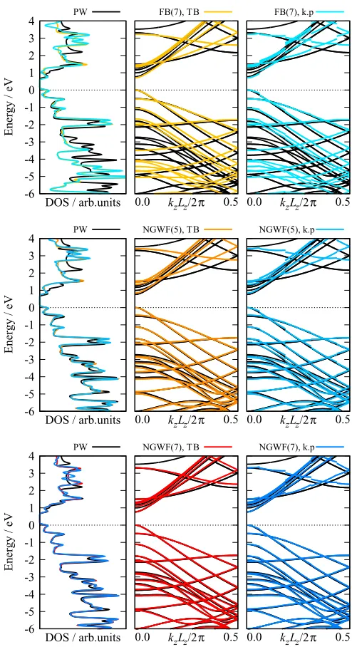
In the first instance, we performed ONETEP calculations for a supercell containing eight repeat units of the CNT and thus 320 atoms. We used four NGWFs per carbon atom. The CASTEP calculation was for the primitive cell, with a Monkhorst-Pack k-point mesh of 1×1×8. The ONETEP supercell band structures were unfolded for comparison with CASTEP. As with the toy model, we wished to consider cases where the basis is of relatively low quality as well as a good calculation setup, and thus considered two scenarios where the basis would be considered poor, namely an NGWF basis which consists of unoptimized FBs but with reasonable localization radii of 7 a0, and a well optimized NGWF basis but with small radii of 5 a0, which are respectively denoted by FB(7) and NGWF(5). This was compared with a good calculation setup with an optimized NGWF basis with radii of 7 a0, denoted by NGWF(7).
The band structures calculated using both methods and associated DOS are plotted in Fig.5. Considering first only the valence states, it is clear that the unoptimized basis is poor, with the band structure showing significant differences with the PW reference, both at the-point and across the BZ. The situation is improved upon optimizing the NGWFs, even for small radii, for which there are only quite small deviations from the PW band structure, while for the calculation with larger NGWF radii there is excellent agreement between the ONETEP and PW band structure. Importantly, the NGWF basis is capable of correctly reproducing the band structure across the whole BZ, despite having only been explicitly optimized at the-point.
For the conduction states, although the final calculation setup shows the smallest errors, in each case there is nonethe-less a visible error compared to the PW result. This is unsur-prising given that, as discussed above, the NGWF optimiza-tion procedure is designed to construct a basis which can ac-curately represent the valence states. Therefore, even though the error is reduced by increasing the NGWF radii, this is not in itself sufficient to guarantee a good basis representation for the empty states. In the following, we therefore also perform band structure calculations using a second set of conduction NGWFs.
-6 -5 -4 -3 -2 -1 0 1 2 3 4
Energy / eV
DOS / arb.units
PW
-6 -5 -4 -3 -2 -1 0 1 2 3 4
Energy / eV
DOS / arb.units
PW
-6 -5 -4 -3 -2 -1 0 1 2 3 4
Energy / eV
DOS / arb.units
PW
0.0 kzLz/2π 0.5
FB(7), TB
0.0 kzLz/2π 0.5
FB(7), k.p
0.0 kzLz/2π 0.5
NGWF(5), TB
0.0 kzLz/2π 0.5
NGWF(5), k.p
0.0 kzLz/2π 0.5
NGWF(7), TB
0.0 kzLz/2π 0.5
NGWF(7), k.p
FIG. 5. Density of states (left) and band structures calculated using the TB (middle) andk·p(right) methods for different setups, compared to the PW reference. The ONETEP setups consist of unoptimized fireballs (FBs) with NGWF radii of 7 a0 (top), and
optimized NGWFs with radii of 5 a0 (middle) and 7 a0 (bottom).
In each case, there were four NGWF functions per carbon atom. For the DOS a Gaussian smearing of 0.05 eV was applied. Each plot has been shifted so that the highest occupied molecular orbital (HOMO) is at zero.
[image:7.590.61.269.59.214.2]-2.5 -2.0 -1.5 -1.0 -0.5 0.0
0.0 0.5
Energy / eV
kzLz/2π NGWF(5), TB, SCBZ
NGWF(5), TB, PBZ
0.0 kzLz/2π 0.5
[image:8.590.40.285.61.207.2]NGWF(5), k.p, SCBZ NGWF(5), k.p, PBZ
FIG. 6. Demonstration of the origin of band discontinuities when using thek·pmethod (right), compared with the continous bands resulting from the TB method (left). The folded supercell (SC) band structure for a supercell of four repeat units is contrasted with the unfolded band structure in the primitive Brillouin zone (PBZ). A single band has been highlighted in black (darker blue) to emphasize the presence of gaps (discontinuities) in the folded (unfolded) band. The plot has been shifted so that the HOMO is at zero.
the unfolded band structure is clearly visible. As expected, no such gaps are present for the TB method and thus the unfolded bands remain smooth and continuous. Furthermore, the shape of the conduction bands is also better calculated with the TB method, for example for the band which is just above 3 eV at the point, the local shape of the bands (i.e., between discontinuities) deviates noticeably from the PW band. This is consistent with the observations from the Kronig-Penney model, where the TB approach resulted in bands with a shape closer to the reference.
It is also interesting to compare the ONETEP band struc-tures with the PW reference in a more quantitative manner. To do so, we calculate the band structures over a dense sampling of k-points and determine the average absolute difference between the PW and ONETEP energies, after first shifting the energy values to account for the difference in HOMO values. This average error is calculated separately for the valence states and for a fixed number of conduction states; the values are given in TableIII. Similar values were
obtained when the energies were compared for only those
k-points that were included in the Monkhorst-Pack mesh for the CASTEP calculation. As expected, the valence errors for the unoptimized basis are significantly higher, with the error decreasing for increasing NGWF radii once the basis is optimized. In all three cases, the conduction errors are significant. Interestingly, the average errors are very similar for the two methods, with k·p worse for the conduction states but otherwise virtually identical for the valence states. Nonetheless, the TB approach is clearly the method of choice, in agreement with the conclusions drawn from the toy model calculations.
A. Conduction states
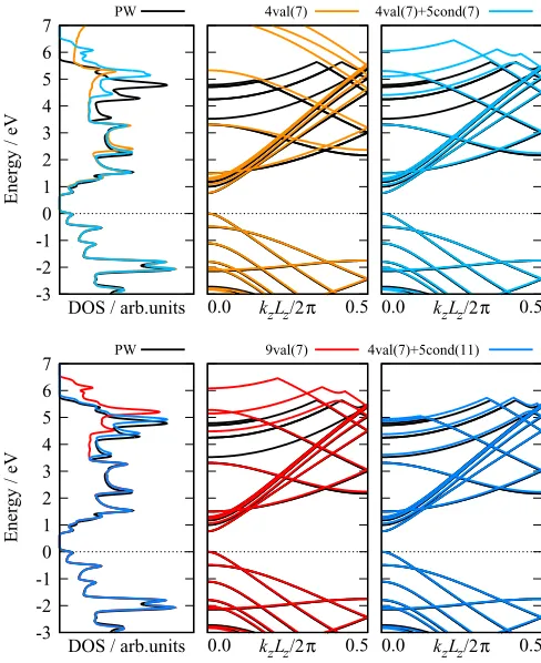
We now investigate in more detail the conduction state band structure. To have the possibility of employing large NGWF radii, we increase the size of the supercell to contain 11 repeat units, otherwise the simulation setup remains the same. In the following, we use only the TB method, since it has proven to be the better choice.
We compare four different calculation setups: two with only valence NGWFs and two with both valence and conduc-tion NGWFs. These combinaconduc-tions were chosen to allow us to compare the varying impacts of increasing the number of valence NGWFs without performing a conduction calculation, adding conduction NGWFs, and increasing the conduction NGWF radii. For shorthand, we use the notationNvval(rv)+
Nccond(rc), where Nv (Nc) is the number of valence (con-duction) NGWFs andrv(rc) denotes the valence (conduction) NGWF radii. The four setups are as follows:
(1) Four valence NGWFs with radii of 7 a0, no conduction NGWFs [4val(7)].
(2) Nine valence NGWFs with radii of 7 a0, no conduction NGWFs [9val(7)].
(3) Four valence NGWFs with radii of 7 a0and 5 conduc-tion NGWFs with radii of 7 a0[4val(7)+5cond(7)].
(4) Four valence NGWFs with radii of 7 a0and 5 conduc-tion NGWFs with radii of 11 a0[4val(7)+5cond(11)].
The number of conduction states to optimize was selected to include all states which are less than 5 eV above the HOMO at the -point, as calculated with CASTEP. A significant
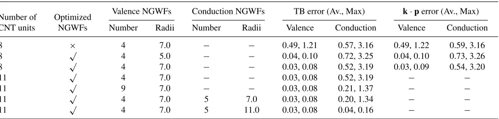
TABLE III. Average and maximum errors across bands andk-points with respect to the PW band structure, in eV. Calculation setups are the same as those used for Figs.5and7. The number of CNT units, whether or not the NGWFs have been optimized, the number of valence and conduction NGWFs per atom, and their respective localization radii are indicated. The valence error is that averaged across all occupied states, while the conduction error has been calculated for the number of unoccupied states for which the calculated PW energy is less than 5.0 eV above the HOMO at thepoint.
Number of Optimized Valence NGWFs Conduction NGWFs TB error (Av., Max) k·perror (Av., Max)
CNT units NGWFs Number Radii Number Radii Valence Conduction Valence Conduction
8 × 4 7.0 − − 0.49, 1.21 0.57, 3.16 0.49, 1.22 0.59, 3.16
8 √ 4 5.0 − − 0.04, 0.10 0.72, 3.25 0.04, 0.10 0.73, 3.26
8 √ 4 7.0 − − 0.03, 0.08 0.52, 3.19 0.03, 0.09 0.54, 3.20
11 √ 4 7.0 − − 0.03, 0.08 0.52, 3.19 − −
11 √ 9 7.0 − − 0.03, 0.08 0.21, 1.37 − −
11 √ 4 7.0 5 7.0 0.03, 0.08 0.20, 1.34 − −
[image:8.590.41.548.621.742.2]-3 -2 -1 0 1 2 3 4 5 6 7
Energy / eV
DOS / arb.units
PW
-3 -2 -1 0 1 2 3 4 5 6 7
Energy / eV
DOS / arb.units
PW
0.0 kzLz/2π 0.5
4val(7)
0.0 kzLz/2π 0.5
4val(7)+5cond(7)
0.0 kzLz/2π 0.5
9val(7)
0.0 kzLz/2π 0.5
[image:9.590.43.287.61.360.2]4val(7)+5cond(11)
FIG. 7. Density of states (left) and band structures calculated using the TB method for different setups, compared to the PW reference. The NGWF setups are given in the figure, whereNvval(rv) denotesNvvalence NGWFs with radiusrv andNccond(rc) denotes
Nc conduction NGWFs with radius rc. A Gaussian smearing of 0.05 eV was applied for the DOS. Each plot has been shifted so that the highest occupied molecular orbital (HOMO) is at zero.
number of additional states (eight times the number actually required) were included in the conduction density kernel in an initial pre-optimization process [56].
The results are plotted in Fig. 7 and the corresponding quantitative errors given in TableIII. For both the ONETEP and PW band structures and DOS, we only depict explicitly optimized conduction states. For 4val(7), the lower energy conduction bands are in relatively good agreement with the PW results, with the largest differences appearing at the BZ boundary. However the higher energy nearly free-electron states, which are equivalent to the weakly bound delocalized states that sit above and below a graphene sheet [61], are completely absent. When the number of NGWFs per atom is increased to nine [9val(7)], the agreement for the low energy states is excellent and there are some free-electron-like states present, however their energies are nonetheless significantly overestimated.
The 9val(7) and 4val(7)+5cond(7) setups have the same number of basis degrees of freedom (same total number of NGWFs and radii) and so can be directly compared. Indeed the band structures are of similar quality, with 4val(7)+5cond(7) showing marginally better agreement on average. However, when the conduction NGWF radii are increased to 11 a0(4val(7)+5cond(11)), the agreement for all
states is markedly improved, with the quantitative difference with the PW band structure at a similar level as for the valence states. As with the valence band structure, it is important to note that a consistent level of accuracy is maintained throughout the BZ.
Given that the accuracy of the 9val(7) and 4val(7)+ 5cond(7) band structures are of similar quality, one might wonder if a conduction calculation is indeed necessary, or if it would also be possible to achieve high quality results by continuing to increase the valence NGWF radii. However, al-though increasing the radii might indeed improve the quality, systematic improvement is not guaranteed, particularly for the higher energy conduction states. The results obtained using the conduction approach, on the other hand, are expected to be at least as good as a valence-only calculation with the same number of degrees of freedom, and in the majority of cases should be significantly better.
V. CONCLUSIONS
In summary, we have presented two methods for calculat-ing band structures uscalculat-ing a local orbital basis set, which are derived fromk·p perturbation theory and TB, respectively. The two methods were initially compared in the context of a one-dimensional model, using a Kronig-Penney potential and two different localized basis sets: a piecewise quadratic nearest neighbor basis and cubic B-splines. Subsequently, the two approaches were compared for a set of optimized local orbitals, referred to as NGWFs, obtained from the ONETEP linear-scaling DFT code for the example of a (10,0) CNT.
For high quality basis sets, i.e., B-splines in the case of the toy model and an optimized set of NGWFs with sufficient degrees of freedom for the ONETEP calculations, band struc-tures generated with the two methods are similar. However, for a lower quality basis, such as the nearest neighbor basis set or unoptimized local orbitals, thek·pstyle method was found to produce unphysical gaps at the BZ boundary. When unfolding band structures obtained from supercell calculations, these gaps translate to discontinuities in the band structure. This problem can arise even for a moderate quality basis set, although the discontinuities are much smaller. The TB-style method guarantees the correct BZ periodicity so that this problem does not occur. Furthermore, when the error with respect to the PW reference is assessed quantititavely, the errors are smaller than or equal to those for the k·p style method. Therefore the TB-style approach is the recommended method for calculating band structures in ONETEP or similar linear scaling approaches.
of freedom, including the use of conduction NGWFs where necessary, the NGWF basis generated by ONETEP forms an excellent basis for band structure interpolation using a TB-style approach.
In the future, it would be interesting to also compare the above results with ONETEP calculations where the impo-sition of the NGWF localization is relaxed in one or more directions, i.e., for partially localized or hybrid Wannier functions. This approach has recently been implemented in ONETEP [62] and is particularly applicable to 2D-periodic systems such as surfaces or interfaces. In particular, such an approach would be expected to result in better convergence for the higher energy conduction states.
Finally, beyond the calculation of band structures, MLWFs are also widely employed as a basis for model Hamiltonian approaches, including TB. Given the above conclusions, the support functions generated from linear-scaling DFT should also be highly suitable for this purpose. In the context of the material considered in this work, an example might be the derivation of TB parameters for defective nanotubes. Given the large system sizes which are accessible to linear-scaling DFT, this approach would also provide an oppor-tunity for validating effective models. For example, one could directly compare large scale DFT calculations with
smaller scale model Hamiltonian calculations to determine whether sufficient degrees of freedom had been included in the model. A similar process can be applied to semiconductors at low doping levels. For example, effective Hamiltonians derived from ONETEP calculations have been used to study sulfur-doped silicon at various (low) defect concentration levels [63].
Underlying data for this paper are available in Ref. [64].
ACKNOWLEDGMENTS
We acknowledge financial support from the UK Engi-neering and Physical Sciences Research Council under the following grants: L.E.R. under Grant No. EP/P504694/1, N.D.M.H. under Grant No. EP/G05567X/1, and L.E.R and P.D.H. under Grant No. EP/J015059/1. The work of G.J.C. was supported by a Nuffield Undergraduate Research Bursary URB/01923/G. P.D.H. acknowledges the support of a Royal Society University Research Fellowship. We are grateful to the UK Materials and Molecular Modelling Hub for computa-tional resources, which is partially funded by EPSRC (Grant No. EP/P020194/1). Calculations were also performed on the Imperial College High Performance Computing Service.
[1] E. L. Shirley,Phys. Rev. B54,16464(1996).
[2] N. Marzari and D. Vanderbilt,Phys. Rev. B56,12847(1997). [3] C. J. Pickard and M. C. Payne,Phys. Rev. B59,4685(1999). [4] D. Prendergast and S. G. Louie, Phys. Rev. B 80, 235126
(2009).
[5] I. Souza, N. Marzari, and D. Vanderbilt, Phys. Rev. B 65, 035109(2001).
[6] N. Marzari, A. A. Mostofi, J. R. Yates, I. Souza, and D. Vanderbilt,Rev. Mod. Phys.84,1419(2012).
[7] A. A. Mostofi, J. R. Yates, Y.-S. Lee, I. Souza, D. Vanderbilt, and N. Marzari,Comput. Phys. Commun.178,685(2008). [8] A. A. Mostofi, J. R. Yates, G. Pizzi, Y.-S. Lee, I. Souza,
D. Vanderbilt, and N. Marzari,Comput. Phys. Commun.185, 2309(2014).
[9] D. R. Hamann and D. Vanderbilt,Phys. Rev. B 79, 045109 (2009).
[10] L. X. Benedict, E. L. Shirley, and R. B. Bohn,Phys. Rev. Lett.
80,4514(1998).
[11] R. D. King-Smith and D. Vanderbilt,Phys. Rev. B47, 1651 (1993).
[12] D. Vanderbilt and R. D. King-Smith,Phys. Rev. B48, 4442 (1993).
[13] R. Resta,Rev. Mod. Phys.66,899(1994).
[14] T. Thonhauser, D. Ceresoli, D. Vanderbilt, and R. Resta,Phys. Rev. Lett.95,137205(2005).
[15] D. Ceresoli, T. Thonhauser, D. Vanderbilt, and R. Resta,Phys. Rev. B74,024408(2006).
[16] I. Souza and D. Vanderbilt,Phys. Rev. B77,054438(2008). [17] W. Zhang, R. Yu, H.-J. Zhang, X. Dai, and Z. Fang,New J.
Phys.12,065013(2010).
[18] A. A. Soluyanov and D. Vanderbilt,Phys. Rev. B83,235401 (2011).
[19] S. Coh, D. Vanderbilt, A. Malashevich, and I. Souza,Phys. Rev. B83,085108(2011).
[20] G. Galli,Curr. Opin. Solid State Mater.1,864(1996). [21] S. Goedecker,Rev. Mod. Phys.71,1085(1999).
[22] D. R. Bowler and T. Miyazaki,Rep. Prog. Phys. 75, 036503 (2012).
[23] N. D. M. Hine, M. Robinson, P. D. Haynes, C.-K. Skylaris, M. C. Payne, and A. A. Mostofi, Phys. Rev. B 83, 195102 (2011).
[24] N. D. M. Hine, P. D. Haynes, A. A. Mostofi, C.-K. Skylaris, and M. C. Payne,Comput. Phys. Commun.180,1041(2009). [25] D. R. Bowler and T. Miyazaki,J. Phys.: Condens. Matter22,
074207(2010).
[26] L. E. Ratcliff, S. Mohr, G. Huhs, T. Deutsch, M. Masella, and L. Genovese,Wiley Interdiscip. Rev.: Comput. Mol. Sci.7,e1290 (2017).
[27] D. J. Cole and N. D. M. Hine,J. Phys.: Condens. Matter28, 393001(2016).
[28] E. Hernández, M. J. Gillan, and C. M. Goringe,Phys. Rev. B
55,13485(1997).
[29] J.-L. Fattebert and J. Bernholc,Phys. Rev. B62,1713(2000). [30] S. Mohr, L. E. Ratcliff, P. Boulanger, L. Genovese, D. Caliste,
T. Deutsch, and S. Goedecker, J. Chem. Phys. 140, 204110 (2014).
[31] S. Mohr, L. E. Ratcliff, L. Genovese, D. Caliste, P. Boulanger, S. Goedecker, and T. Deutsch,Phys. Chem. Chem. Phys.17, 31360(2015).
[32] C.-K. Skylaris, A. A. Mostofi, P. D. Haynes, O. Diéguez, and M. C. Payne, Phys. Rev. B 66, 035119 (2002).
[34] C.-K. Skylaris, P. D. Haynes, A. A. Mostofi, and M. C. Payne, J. Chem. Phys.122,084119(2005).
[35] G. C. Constantinescu and N. D. M. Hine,Phys. Rev. B91, 195416(2015).
[36] N. R. Wilson, P. Nguyen, K. Seyler, P. Rivera, A. J. Marsden, Z. P. L. Laker, G. C. Constantinescu, V. Kandyba, A. Barinov, N. D. M. Hine, X. Xu, and D. H. Cobden,Sci. Adv.3,e1601832 (2017).
[37] G. C. Constantinescu and N. D. M. Hine,Nano Lett.16,2586 (2016).
[38] E. Kane,Semicond. Semimet.1,75(1963).
[39] C. J. Pickard and M. C. Payne,Phys. Rev. B62,4383(2000). [40] P. D. Haynes, C.-K. Skylaris, A. A. Mostofi, and M. C. Payne,
Phys. Status Solidi B243,2489(2006). [41] W. Kohn,Phys. Rev. Lett.76,3168(1996). [42] R. McWeeny,Rev. Mod. Phys.32,335(1960).
[43] X.-P. Li, R. W. Nunes, and D. Vanderbilt,Phys. Rev. B47, 10891(1993).
[44] M. S. Daw,Phys. Rev. B47,10895(1993).
[45] R. W. Nunes and D. Vanderbilt, Phys. Rev. B 50, 17611 (1994).
[46] P. D. Haynes, C.-K. Skylaris, A. A. Mostofi, and M. C. Payne, J. Phys.: Condens. Matter20,294207(2008).
[47] P. D. Haynes and M. C. Payne, Phys. Rev. B 59, 12173 (1999).
[48] O. F. Sankey and D. J. Niklewski,Phys. Rev. B40,3979(1989). [49] A. A. Mostofi, P. D. Haynes, C.-K. Skylaris, and M. C. Payne,
J. Chem. Phys.119,8842(2003).
[50] D. Baye and P.-H. Heenen,J. Phys. A19,2041(1986). [51] K. Varga, Z. Zhang, and S. T. Pantelides,Phys. Rev. Lett.93,
176403(2004).
[52] C.-K. Skylaris, A. A. Mostofi, P. D. Haynes, C. J. Pickard, and M. C. Payne,Comput. Phys. Commun.140,315(2001). [53] A. A. Mostofi, C.-K. Skylaris, P. D. Haynes, and M. C. Payne,
Comput. Phys. Commun.147,788(2002).
[54] C.-K. Skylaris, P. D. Haynes, A. A. Mostofi, and M. C. Payne, J. Phys.: Condens. Matter17,5757(2005).
[55] P. D. Haynes, C.-K. Skylaris, A. A. Mostofi, and M. C. Payne, Chem. Phys. Lett.422,345(2006).
[56] L. E. Ratcliff, N. D. M. Hine, and P. D. Haynes,Phys. Rev. B
84,165131(2011).
[57] L. E. Ratcliff and P. D. Haynes,Phys. Chem. Chem. Phys.15, 13024(2013).
[58] L. Kleinman and D. M. Bylander, Phys. Rev. Lett.48, 1425 (1982).
[59] S. J. Clark, M. D. Segall, C. J. Pickard, P. J. Hasnip, M. I. J. Probert, K. Refson, and M. C. Payne,Z. Kristall.220, 567 (2005).
[60] J. P. Perdew, K. Burke, and M. Ernzerhof,Phys. Rev. Lett.77, 3865(1996).
[61] M. Houssa, A. Dimoulas, and A. Molle (eds.) 2DMaterials for Nanoelectronics CRC Press(Taylor & Francis Group, Boca Raton, FL, 2016).
[62] A. Greco, Development and Application of First-Principles Methods for Complex Oxide Surfaces and Interfaces, Ph.D. Thesis, Imperial College London, 2017.
[63] E. G. Carnio, N. D. M. Hine, and R. A. Römer, arXiv:1710.01742v2.