Squibs: Evaluating Human Pairwise Preference Judgments

Preference Judgments

Mark Dras

Centre for Language Technology Macquarie University

Human evaluation plays an important role in NLP, often in the form of preference judgments. Although there has been some use of classical non-parametric and bespoke approaches to evaluat-ing these sorts of judgments, there is an entire body of work on this in the context of sensory discrimination testing and the human judgments that are central to it, backed by rigorous statistical theory and freely available software, that NLP can draw on. We investigate one approach, Log-Linear Bradley-Terry models, and apply it to sample NLP data.

1. Introduction

Human evaluation is a key aspect of many NLP technologies. Automatic metrics that correlate with human judgments have been developed, especially in Machine Transla-tion, to relieve some of the burden. Neverthess, Callison-Burch et al. (2007) note in their meta-evaluation that in MT they still “consider the human evaluation to be primary.” Whereas MT has traditionally used a Likert scale score for the criteria of adequacy and fluency, this meta-evaluation noted that these are “seemingly difficult things for judges to agree on”; consequently, asking judges to express a preference between alternative translations is increasingly used on the grounds of ease and intuitiveness. Further, where the major empirical results of a paper are from automatic metrics, it is still useful to supplement them: As two examples, Collins, Koehn, and Kucerova (2005) and Lewis and Steedman (2013), in addition to a metric-based evaluation, present human judg-ments of preferences for their systems with respect to a baseline (Fig. 1). For results in published work, the reader is typically left to draw inferences from the numbers. For the data in Figure 1, is there a strong preference for the non-baseline system overall, or do null preferences count against that? Is anything about the results statistically significant? There has been work in various areas of NLP in assessing statistical significance of human judgment results. However, to our knowledge, the field has not taken advantage of a body of work dedicated to analyzing human preferences—predominantly in the context of sensory discrimination testing, and consequent consumer behavior—which is supported by a great deal of statistical theory. It is linked to the mixed-effect models that are increasingly prominent in psycholinguistics and elsewhere, it has associated freely availableRsoftware, and it permits questions like the following to be asked: Can we say that the judges are expressing a preference at all, as opposed to no preference? Is there an effect from judge disagreement or inconsistency?

∗Department of Computing, Macquarie University, NSW 2109, Australia. E-mail:[email protected].

Submission received: 10 April 2014; accepted for publication: 18 July 2014.

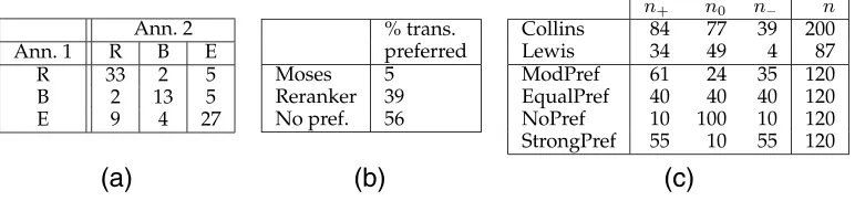
Figure 1

(a) Results for two human judges (annotators) in Collins et al. (2005), Table 2. R gives counts corresponding to preferences for reordered translation system; B, preferences for baseline; E, no preference. (b) Results for human judges for baseline Moses versus cluster-based reranker in Lewis and Steedman (2013), Table 5. (c) Count data of pairwise preferences from Collins et al. (2005) and Lewis and Steedman (2013) plus artificial data.

We describe our sample data (Section 2), sketch a classical non-parametric approach (Section 3) and discuss the issues that arise from this, and look at some of the approaches used in MT (Section 4). We then (Section 5) introduce ideas from human sensory pref-erence testing, where we review log-linear Bradley-Terry models of prefpref-erences, and apply this to our data, including discussion of ties, of subject effects, and of multiple pairwise comparisons.

2. Two Data Sets

Single Pairwise Comparison.Our basic single pairwise comparisons are those presented in Figure 1(a) and (b). Figure 1(c) contains the counts we will be using in later analysis: We refer to counts in favor of the new system byn+, those in favor of the baseline byn−,

and those reflecting no preference asn0; the Lewis and Steedman results were over 87 pairwise judgments. We add some further artificial data to illustrate how the Log-Linear Bradley-Terry (LLBT) models of Section 5 behave in accordance with intuition for data where the conclusion should be clear. These comprise a distribution with a moderate preference for +over−and not too many null preferences (ModPref), a distribution of equal preferences over all three categories (EqualPref), a distribution with mostly null preferences and equaln+ andn−(NoPref), and a distribution with very few null

preferences (StrongPref).

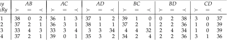
Table 1

Artificial pairwise MT data for four systemsA,B,C,D.xRyrepresents whetherxis preferred to

y(xy), the reverse (x≺y), or no preference (x=y), for four judges J1 . . . J4.

xy AB AC AD BC BD CD

xRy = ≺ = ≺ = ≺ = ≺ = ≺ = ≺

J1 38 0 2 36 1 3 37 1 2 39 1 0 0 2 38 3 0 37

J2 37 2 1 36 3 1 38 1 1 37 2 1 2 2 36 1 0 39

J3 33 4 3 33 3 4 3 3 34 4 4 32 2 4 34 1 0 39

J4 37 2 1 39 0 1 35 3 2 34 2 4 2 2 36 3 1 36

3. Classical Non-Parametric Methods

A classical approach to evaluating preferences is the non-parametric sign test (Sprent and Smeeton 2007). The first issue in applying this test here is ties, or expressions of no preference—these are often ignored when the proportion of ties is small, but for our typical examples of Figure 1, this is not true. Randles (2001) observes, regarding the approach most widely recommended by textbooks of just ignoring ties, that “the constrained number of possible p values and its ‘elimination of zeroes’ has caused concern and controversy through the years.” Randles (2001) and Rayner and Best (2001, chapter 2), reviewing several approaches to handling ties, both advocate splitting ties in various ways depending on the problem setting, for (in Randles’s characterization) “it is desirable that zeros have a conservative influence on declaring preference, but not to the same degree as negative responses.” The key point is that modeling of ties explicitly can be important, although there is no consensus on how this should be done; no approach apart from ignoring ties appears to be in widespread use. The second issue with the sign test is that of multiple judges, where data points are related (e.g., the same items are given to all judges). The Friedman test (Sprent and Smeeton 2007, Section 7.3.1) can be viewed as an extension that can be applied to multiple subjects ranking multiple items (see Bi 2006, Section 5.1.3, for an example). However, Francis, Dittrich, and Hatzinger (2010) note that

[the Friedman test] simply examines the null hypothesis that the median ranks for all items are equal, and does not consider any differences in ranking between respondents. . . . Moreover, if the Friedman test rejects the null hypothesis, no quantitative interpretation, such as the odds of preferring one item over another, is provided. [Further, this] fail[s] both to consider the underlying psychological mechanism for ranking, and to formulate correct statistical models for this mechanism.

4. Methods in Machine Translation

et al. 2008) took the same approach, but noted that in ranking, “[h]ow best to treat these is an open discussion, and certainly warrants further thought,” in particular because of ties “further complicating matters.” Pado et al. (2009) modified the system-level predictions approach to become “tie-aware,” and noted that that this “makes a considerable practical difference, improving correlation figures by 5–10 points.” At around the same time Vilar et al. (2007) examined the use of pairwise comparisons in MT evaluation. They pose the problem as one where, given an order relationship

is-better-thanbetween pairs of systems, the goal is to find an ordering of all the systems: They see this as the fundamental computer science problem of sorting. They define an aggregate evaluation score for comparing systems, estimating expected value and standard error for hypothesis testing. However, in aggregating this way information about ties is lost.

Bojar et al. (2011) critique the earlier WMT evaluations, citing issues with the ignoring of non-top ranks (noted in Section 3 herein also), with ties and also with interannotator agreement. Lopez (2012) extends the analysis of Bojar et al. and casts the problem as “finding the minimum feedback arc set in a tournament, a well-known NP-complete problem.” He advocates using the pairwise rankings themselves, rather than aggregate statistics like Vilar et al. (2007), and aims to minimize the number of violations among these. Koehn (2012) evaluates empirically the approaches of both Bojar et al. (2011) and Lopez (2012), with a focus on determining which systems are statistically distinguishable in terms of performance, defining confidence bounds for this purpose.

Hopkins and May (2013) recently advocated a focus on finding the extent to which particular rankings could be trusted. They proposed a model based on Item Response Theory (IRT), which underlies many standardized tests. They draw an analogy with judges assessing students on the basis of an underlying distribution of the student’s ability, with items authored by students having a quality drawn from the student’s ability distribution. They note in passing that a Gaussian parameterization of their IRT models resembles Thurstone and Bradley-Terry models; this leads us to the topic of Section 5.

Overall, then, there are ongoing discussions about what kind of analysis is appro-priate for preference judgments. Some of this involves moderately heavy-duty compu-tation for bootstrapping; this is suitable for large-scale WMT evaluations with dozens of competing systems, but perhaps less so for the scenarios we envisage in Section 1. More-over, examining what techniques other fields have developed could be useful, especially when they come with ready-made, easy-to-use tools for smaller-scale evaluation.

5. Preferences and Log-Linear Bradley-Terry Methods

In a basic BT model, the probability that objectj(Oj) is preferred to objectk(Ok) from

a set ofJobjects in a particular pairwise comparisonjkis given byp(OjOk|πj,πk)= πj

πj+πk for allj=k, whereπjandπkare non-negative “worth” parameters describing the

location of the object on the scale of preferences for some attribute. Fornobjects, there will ben₂pairwise comparisons.

Log-Linear Models. It is now standard to fit BT models as log-linear models (Agresti 2007, for example), which allows them to be treated in a uniform way with much of modern statistical analysis. Log-linear models are a variety of generalized linear models (GLM), as is, for example, the logistic regression used throughout NLP. GLMs consist of a random component that identifies the response variableYand selects a probability distribution for it; a systematic component that specifies some linear combination of the explanatory variablesxi; and a link functiong(·) applied to the meanμofYrelating μto this linear combination. They thus have the formg(μ)=α+β1x1+. . .+βkxk. For

log-linear models, the response variables are counts that are assumed to follow a Pois-son distribution, and the link function isg(μ)=log(μ) (compare logistic regression’s

g(μ)=log₁₋μ_μ). As an example, Y might be counts of people who hold some belief, and the variousximight be gender, socioeconomic status, and so forth. GLMs are a key tool for modern categorical data analysis, Agresti (2007, p. 65) noting that using models rather than the non-parametric approaches of Section 3 has several benefits:

The structural form of the model describes the patterns of association and interaction. The sizes of the model parameters determine the strength and importance of the effects. Inferences about the parameters evaluate which explanatory variables affect the response variableY, while controlling effects of possible confounding variables. Finally, the model’s predicted values smooth the data and provide improved estimates of the mean ofYat possible explanatory variable values.

In a log-linear model, intuitive log-odds interpretations of making one response relative to another can be derived from the parameters. (Typically, software chooses a reference parameter and other parameter values are relative to that.) Statistical signif-icance scores and standard errors can be calculated for these parameters. In addition, GLMs allow for testing of model fit. There are various model choices (e.g., should we include ties? should we include terms representing interactions?) and goodness-of-fit tests can assess the alternatives (see, e.g., Agresti 2007, Section 7.2.1). The model with a separate parameter for each cell in the associated contingency table is called thesaturated model, and fits the data perfectly, making it a suitable comparator for alternatives. Deviance is a likelihood ratio statistic comparing a proposed model to the saturated one, allowing a test of the hypothesis that parameters not included in the model are zero, via goodness of fit tests; large test statistics and small p-values provide evidence of model lack of fit.

Models with Ties. To set out the representation of LLBT models, we follow the for-mulation of Dittrich and Hatzinger (2009). Let n(jk) be the number of comparisons between objects j and k; and let Y(jk)j be the number of preferences for object j with

respect to k (similarly, Y(jk)k). The outcome of a paired comparison experiment can

also be regarded as a₂J×Jincomplete two-dimensional contingency table: There are _J

2

follow a binomial (more generally, multinomial) distribution. The expected number of preferences of object jwith respect to objectkis denotedm(jk)j and given byn(jk)p(jk)j,

with p(jk)j the binomial probability. So far this is only for binary preferences; there are

various ways to account for ties. We describe the approach of Davidson and Beaver (1977), which appears quite widely used, where there is a common null preference effect for all pairwise comparisons. Then

logm(jk)j=μ(jk)+λOj −λOk

logm(jk)0=μ(jk) +γ logm(jk)k=μ(jk)−λOj +λOk

(1)

where theμ’s are “nuisance” parameters that fix then(jk)marginal distributions, and the

λO_{’s represent object parameters,m}

(jk)0is the expected number of null preferences for pair (jk), andγis the undecided effect. The object parameters are related to the worth parameters of the original definition by logπ=2λO: These represent the log-odds.

In addition to the theoretical reasons for using LLBTs for modeling pairwise com-parisons, a key benefit is the availability of packages inRfor doing the modeling. Two candidates allowing a variety of sophisticated models are by Turner and Firth (2012) and Hatzinger and Dittrich (2012); we use the latter as the current version of the former does not handle ties. We first apply the model described by Equations (1) to the single pairwise data with ties from Section 2 usingR. We refer the reader to the associated data bundle1 _{for the full output; we only excerpt it in the discussion below. Immediately} following is a snippet of the Routput for the ModPref data from Figure 1. o1 is the variableλO

j for the + category,o2for the – category,g1for the null preferences.

Estimate Std. Error z value Pr(>|z|)

o1 0.2778 0.1060 2.620 0.0088 **

o2 0.0000 NA NA NA

g1 -0.6551 0.2300 -2.848 0.0044 **

---Signif. codes: 0 ‘***’ 0.001 ‘**’ 0.01 ‘*’ 0.05 ‘.’ 0.1 ‘ ’ 1 Residual deviance: -6.6614e-15 on 0 degrees of freedom

In the R output, o2 is the reference object, with parameter value set to zero; the negative value of the estimate forg1combined with its statistical significance says that there is a strong tendency for an expression of preference. The positive value of theo1 parameter and its significance indicate that the + group is strongly preferred: The odds in favor of this group with respect to the – group is exp(2×0.2778)=1.74 to 1. Relating this to the description of the data in Section 2, then, there is a strong preference for trans-lations by the proposed system relative to the baseline, even taking into account null preferences. The LLBT model confirms that even small data sets like this can produce meaningful and statistically significant results. For the other artificial preference data of Figure 1, the parameters behave as expected: for EqualPref, parameter estimates are all zero, signifying that they all have the same odds; for NoPref, the positiveg1indicates a strong tendency towards no preference; for StrongPref, the negative g1 indicates a strong tendency towards some preference, but with + or – equally likely. Note that all of these are saturated models: there are three objects and three parameters, so the model fits perfectly (indicated also by zero residual deviance). When we apply them

to the real count data of Figure 1 (c), the results indicate that for the Collins et al. data there is a weak to moderate tendency not to choose (g1estimate 0.303, p = 0.0432), but, given that, there is a significant (0.0001) preference in favor of the reordered system. For the Lewis and Steedman results, the model gives similar results, albeit with a much stronger disposition to null preferences. In the data bundle we also carry out the sign test ignoring ties for each data set for comparison; it gives the same results in each case for the relation of + than –, but does not allow an evaluation of the effect of ties.

We now apply the model described by Equations (1) to the multiple pairwise data of Table 1. In theRoutput, the four systems A, B, C, D correspond to objectso1,o2,o3,o4, andg1again to null preferences. As per the overview of the MT data in Section 2, there is little undecidedness (large negativeg1). The coefficients show that objecto1(system A) is most preferred, followed byo4 (D), theno2(B) ando3 (C). Note also that in this case, the model is not saturated: There is a non-zero residual deviance. As mentioned, log-linear models can be compared in terms of goodness of fit: Dittrich, Hatzinger, and Katzenbeisser (1998) and Dittrich and Hatzinger (2009) discuss this in some detail for LLBT models. Chi-squared statistics can be used to assess goodness of fit based on the residual deviance; the degrees of freedom (d.f.) equal the number of cell counts minus the number of model parameters; both deviance and d.f. are given in theRoutput. For this data deviance is 30.646 on 8 d.f., whereas by contrast if the ties (g1) are left out, it is 221.22 on 9 d.f. A chi-squared test would establish the goodness of fit for each model; but even without consulting the test it can be seen that leaving out the one parameter related to ties (1 d.f.) gives a seven-fold increase in deviance, so clearly inclusion of ties produces a much better model.

Introducing Subject Covariates.The model can also incorporate a range of other factors, a possibility not easily open to non-parametric methods. The one we look at here is the notion of a categorical covariate, introduced into LLBT models in Dittrich, Hatzinger, and Katzenbeisser (1998): This allows the objects (items) to vary with characteristics of the subject (judge). Many types of subject covariates could be added, grouping subjects by native language of the speaker, source of judges (e.g., Mechanical Turk, university), and so forth. Here we add just one, the identity of the subject. (Typically in a GLM this would be a random effect; we treat it as a covariate just for our simple illustration.) We define our categorical covariateS to have levelsl,l=1, 2,. . .,L. Let m(jk)j|l be the

expected number of preferences for object j with respect to object k for subjects in covariate classl. The log-linear representation is then as follows:

logm(jk)j|l =μ(jk)l +λjO −λOk +λlS+λOSjl −λOSkl

logm(jk)0|l =μ(jk)l +λSl +γ

logm_(jk)k|l =μ(jk)l −λjO +λOk +λlS−λOSjl +λOSkl

(2)

As do Dittrich and Hatzinger (2009), we define a reference group, with the λO_j ’s representing the ordering for that group; the orderings for other groups are obtained by adding theλOS_jl ’s specific to grouplto theλO_l ’s for the reference group.μ(jk)l andλSl

are again “nuisance” parameters, the latter representing the main effect of the subject covariate measured on the lth level; λOS

jl ’s are the (useful) subject-object interaction

parameters describing the effect of the subject covariate on the preference for object

of this article to discuss but covered in Dittrich, Hatzinger, and Katzenbeisser (1998). The broad interpretations to draw from the output are that interactionso1:SUBJ3 and o2:SUBJ3are large and significant, and contribute to the model, unlike any others. These correspond to the different pairwise rankings given by judge J3 to system A (relative to D) and to B (relative to C): This is how subject effects are indicated in these LLBT models.

There are many other extensions to these models. Cattelan (2012) gives a state-of-the-art overview of such extensions across a range of approaches, with an emphasis on dependent data. We only note two extensions here that are incorporated into prefmod and relevant to NLP. Withcategorical object covariates, items can be grouped as well, to investigate effects of grouping there, for example, different origins for translation sources. Withnon-pairwise rankings, judges can rank over more than two elements, as in the standard WMT evaluations, although this needs a special treatment in the models.

6. Conclusions

We have looked at the sort of (pairwise) preference data that is encountered often in NLP. A particular characteristic of NLP data is that ties or undecided results may be frequent, and there is often a concern with inter-judge consistency. Reviewing classical non-parametric approaches, we note the opinion that it is important to model ties, and also note that approaches to looking at subject (judge) effects have several issues, such as a lack of quantitative interpretation of results. Among NLP approaches, especially within MT, new techniques are still being derived, which could benefit from views from outside the field. What we present are techniques from the field of sensory preference evaluation, where there has been a long history of development by statistics researchers. Recently, log-linear models have attracted attention. Applying them to sample data, we find that they provide the sort of information and uniform framework for analysis that NLP researchers could find useful. Given both extensive theoretical underpinings and freely available statistical software, we recommend LLBT models as a potential tool.

References

Agresti, Alan. 2007.An Introduction to Categorical Data Analysis. John Wiley, 2nd edition.

Bi, Jian. 2006.Sensory Discrimination Tests and Measurements: Statistical Principles, Procedures and Tables. Blackwell, Oxford, UK.

Bojar, Ondˇrej, Miloˇs Ercegovˇcevi´c, Martin Popel, and Omar Zaidan. 2011. A grain of salt for the WMT manual evaluation. In

Proceedings of WMT, pages 1–11.

Bradley, Ralph and Milton Terry. 1952. Rank analysis of incomplete block designs, I. The method of paired comparisons.

Biometrika, 39:324–345.

Callison-Burch, Chris, Cameron Fordyce, Philipp Koehn, Christof Monz, and Josh Schroeder. 2007. (Meta-) Evaluation of machine translation. InProceedings of WMT, pages 136–158.

Callison-Burch, Chris, Cameron Fordyce, Philipp Koehn, Christof Monz,

and Josh Schroeder. 2008. Further meta-evaluation of machine translation. InProceedings of WMT, pages 70–106.

Cattelan, Manuela. 2012. Models for paired comparison data: A review with emphasis on dependent data.Statistical Science, 27(3):412–423.

Collins, Michael, Philipp Koehn, and Ivona Kucerova. 2005. Clause restructuring for statistical machine translation. InProceedings of ACL, pages 531–540.

Davidson, R. R. and R. J. Beaver. 1977. On extending the Bradley-Terry model to incorporate within-pair order effects.

Biometrics, 33:693–702.

Dittrich, Regina and Reinhold Hatzinger. 2009. Fitting loglinear Bradley-Terry models (LLBT) for paired comparisons using the R package prefmod.

Dittrich, Regina, Reinhold Hatzinger, and W. Katzenbeisser. 1998. Modelling the effect of subject-specific covariates in paired comparison studies with an application to university rankings.

Journal of the Royal Statistical Society, Series C: Applied Statistics,

47:511–525.

Francis, Brian, Regina Dittrich, and Reinhold Hatzinger. 2010. Modeling heterogeneity in ranked responses by nonparametric maximum likelihood: How do Europeans get their scientific knowledge?The Annals of Applied Statistics, 4(4):2181–2202.

Hatzinger, Reinhold and Regina Dittrich. 2012. prefmod: A package for modeling preferences based on paired comparisons, rankings, or ratings.Journal of Statistical Software, 48(10):1–31.

Hopkins, Mark and Jonathan May. 2013. Models of translation competitions. InProceedings of ACL, pages 1,416–1,424.

Koehn, Philipp. 2012. Simulating human judgment in machine translation evaluation campaigns. InProceedings of IWSLT, pages 179–184.

Lawless, Harry T. and Hildegarde Heymann. 2010.Sensory Evaluation of Food: Principles and Practices. Springer, New York, NY 2nd edition.

Lewis, Mike and Mark Steedman. 2013. Unsupervised induction of cross-lingual

semantic relations. InProceedings of EMNLP, pages 681–692.

Lopez, Adam. 2012. Putting human assessments of machine translation systems in order. InProceedings of WMT, pages 1–9.

Pado, Sebastian, Michel Galley, Dan Jurafsky, and Christopher D. Manning. 2009. Robust machine translation evaluation with entailment features. InProceedings of ACL / AFNLP, pages 297–305.

Randles, Ronald H. 2001. On Neutral Responses (zeros) in the sign test and ties in the Wilcoxon-Mann-Whitney test.The American Statistician, 55(2):96–101. Rayner, J. C. W. and D. J. Best. 2001.A

Contingency Table Approach to Nonparametric Testing. Chapman and Hall/CRC, Boca Raton, FL.

Sprent, Peter and Nigel Smeeton. 2007.

Applied Nonparametric Statistical Methods. Chapman and Hall, London, UK. Thurstone, L. L. 1927. A law of comparative

Judgement.Psychological Review, 34:278–286.

Turner, Heather and David Firth. 2012. Bradley-Terry Models in R: The BradleyTerry2 Package.Journal of Statistical Software, 48(9):1–21.