Abstract—In this study, we extend on work on the PtRNASS
algorithm for which we previously only understood the defined maximum region in each substructure. We subsequently discovered another important factor, namely the fact that two results can be affected by a different combination of parameters. All tRNAs are characterized by structures resembling cloverleaves and have lengths mostly within 63-200 bases. Moreover, the sequence usually can be folded into more than one structure prediction. The limitations of these substructures mainly affect computational speed whereas the number of base-pairings achieved mainly affects the algorithm sensitivity. These parameters affect one another. For example, increasing the D-Loop parameter may reduce the length of one or more substructures, thus requiring a suitable combination of these parameters which we determine with a CPSO algorithm. The results provide will allow biologists and researchers to more efficiently locate the tRNA gene.
Index Terms—tRNA Secondary Structure, Particle Swarm
Optimization, Chaos, Parameter Optimization.
I. INTRODUCTION
nderstanding non-coding RNA is very important in terms of the function or role of organisms in cells. In order to understand the functions, RNA has to be constructed as its own stable secondary structure. All transfer RNA (tRNA) molecules can recognize the codons triplet in messenger RNA (mRNA) and carry the respective amino acid to the protein-building machinery. Recent research suggests that the conserved structure in tRNA is involved in some of the earliest and the most profound evolutionary events [1], [2]. Thus, tRNA is an important subject for evolutionary research.
Fig. 1 illustrates tRNA’s secondary structure. The first line shows a predicted tRNA sequence in which the introns and extra bases of the non-numbering system [3] are represented in lower-case letters, and the “GTA” represents the anticodon (see Fig. 1 inset). The second line shows tRNA’s predicted secondary structure with the nested > and < symbols representing the stacked pairings. The four stacked pairs include acceptor stem (A-stem), dihydrouridine stem
L.Y. Chuang is with the Department of Chemical Engineering, I-Shou University , 84001 , Kaohsiung, Taiwan (E-mail: [email protected]) Y.D. Lin is with the Department of Electronic Engineering, National Kaohsiung University of Applied Sciences, 80778, Kaohsiung, Taiwan (E-mail: [email protected])
C.H. Yang is with the Department of Electronic Engineering, National Kaohsiung University of Applied Sciences, 80778, Kaohsiung Taiwan (phone: 886-7-3814526#5639; E-mail: [email protected]). He is also with the Network Systems Department, Toko University, 61363, Chiayi, Taiwan. (E-mail: [email protected]).
(D-stem), anticodon stem (C-stem) and TΨC stem (T-stem), in which their respective general base-pairing length are 7, 4, 5 and 5. The general lengths of the four types of hairpin loops, i.e., TΨC (T-loop), variable (V-loop), anticodon (C-loop), and dihydrouridine (D-loop), are 7, 5, 7 and 8, respectively. The intron may sometimes hide within a C-stem, and it always resides at sequence positions 37 and 38. Table I lists the constraint A, which was found through observation of the characteristics of the irregular tRNA structures and will be optimized in this study.
In previous work we developed a tRNA prediction algorithm [4], [5]. The objective of the current research is to optimize the limited parameters for the regions of tRNA substructures and the minimum numbers of resulting base-pairings, in which they are the loosest limits, as shown in Table I. However, many interactions exist among the parameters, and each parameter has the potential to cause a false prediction. Indeed, all the known tRNAs, which are correctly predicted by our proposed algorithm, are predicted with certainty through the loosest limiting parameters. However, the volume of unnecessary computations also increased, resulting in increased search time. The total number of parameter combinations is 614,718,720, i.e., 2 (A-stem) × 2 (AD-gap) × 11 (D-loop) × 3 (DC-gap) × 28(V-loop) × 6 (T-loop) × 7 (A-stem base-pairing achieved) × 5 (D-stem base-pairing achieved) × 6 (C-stem base-pairing achieved) × 6 (T-stem base-pairing achieved) ×22 (All-stems base-pairing). For our purposes, the best combination has to satisfy all known tRNAs from the Sprinzl database, and should also require fewer computations to predict the tRNA secondary structure. However, finding a suitable parameter to limit tRNA prediction is a key point in the accurate recognition of the tRNA secondary structure. In our research, we used the Chaotic Particle Swarm Optimization (CPSO) algorithm to acquire an optimal parameter from among the large permutation of potential parameter combinations. The resulting parameter successfully achieved our goal for limited-parameter optimization.
Limited-Parameter Optimization for PtRNASS
using Chaotic Particle Swarm Optimization
Li-Yeh Chuang, Yu-Da Lin, and Cheng-Hong Yang, Member, IAENG
Fig.1 tRNA cloverleaf diagram. The illustration shows all substructures of a complete tRNA sequence with primary and secondary structures which include base pairings and loop structures. The “Anticodon” is shown as a block within the C-loop structure, i.e., GTA. The line “Seq.” is a predicted tRNA sequence, in which the introns and extra bases of non-numbering systems are printed in lower-case letters. The next line (Pair) displays the folding of the tRNA with the predicted secondary structure, using the nested > and < symbols to represent based pairings.
I. METHOD
A. Particle Swarm Optimization (PSO)
Particle swarm optimization (PSO) was developed by Kennedy and Eberhart in 1995 [6] as an evolutionary algorithm based on population stochastic optimization techniques. PSO simulates the social behavior of organisms, such as flocks of birds or schools of fish. In PSO, each individual bird within the flock can be candidate for the solution, and PSO identifies which candidate is a particle in the search space. Each particle can make use of its memory and knowledge gained through the particle, thus finding the best solution for the whole swarm. Each particle contains two important properties: (i) its fitness value, which is evaluated with a designed fitness function, and (ii) its velocity, which affects the movement of the particle. During the search, each particle adjusts its position according to its own experience and the experience of a neighboring particle that has achieved the current best position. Other particles can then follow the current best particle in the search space. The operation is iterated until a predefined number of iterations are completed.
In PSO, the position of the ith particle can be represented as
xi = (xi1, xi2, …, xiD), in which D represents the dimensions of
the search space. The velocity of the ith particle can be represented as vi = (vi1, vi2, …, viD). The position X and
velocity V of a particle is respectively confined within [Xmin, Xmax]D and [Vmin, Vmax]D. The best currently visited position of the ith particle is denoted as its individual best position pi =
(p , p , …, p ), referred to as pbest. On achieving the best
fitness amongst all individuals, pbesti is denoted as the
global best position g = (g1, g2, …, gD), or gbest. In PSO, the
position and velocity of the ith particle are updated in the swarm via pbesti and gbest. In PSO, the parameters w, r1 and
r2 are the key factors affecting convergence behavior [7], [8]. The w controls the balance between the global exploration and the local search ability. A large w favors global search, whereas a small w favors local search. For this reason, a w that linearly decreases from 0.9 to 0.4 throughout the search process is widely used [9].
B. Chaotic Particle Swarm Optimizaiton (CPSO)
Chaos has ergodic and stochastic properties; it can be described as a bounded nonlinear system with deterministic dynamic behavior [10]. The “butterfly effect” strategy holds that a small variation in an initial variable will result in huge differences in results after multiple iterations. Mathematically, chaos is random and unpredictable, yet it also possesses an element of regularity. Since logistic maps are frequently used as chaotic behavior maps, the chaotic sequences can be quickly generated and easily stored without need for storing long sequences [11]. In CPSO, sequences generated by a logistic map are substituted for the random parameters r1 and r2 in PSO.
C. The Usages of Database
testing the prediction sensitivity. It contains the most comprehensive tRNA sequences from a wide variety of organisms, and are divided into three different sets of tRNA genes, from Archaea (161 sequences), Bacteria (686 sequences) and Eukaryota (443 sequences).
D. Application of CPSO Algorithm
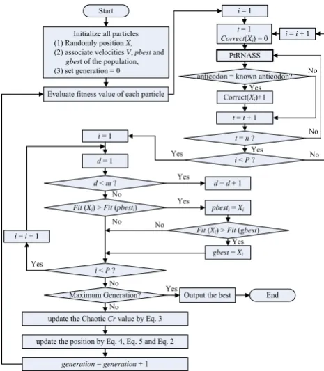
In the CPSO algorithm, each particle represents a candidate solution to the problem. Detailed steps are shown below and in Fig. 2.
a) Initialize the particle swarm
First, all particles P = (AS, ADg, DL, DCg, VL, TL, ASp, DSp, CSp, TSp, AllSp) are randomly generated without duplicates as the initial particle swarm and their values are limited as in Fig. 3. We aim to understand their minimum or maximum length within the substructures. The VL is designed to find V-loop’s maximum length, while the AS, ADg, DL, DCg, and TL are designed to find its minimum length. The ASp, DSp, CSp, TSp, AllSp are designed to find the particle’s optimal limitations allowed for the minimum number of base-pairing. In this step, we intentionally set the loosest limitations to the parts of particles to both exploit all the loosest limiting positions from the designed particles and to guide or expand the particles to promising new areas.
Initialize all particles (1) Randomly position X, (2) associate velocities V, pbest and
gbest of the population, (3) set generation = 0
End Evaluate fitness value of each particle
Maximum Generation? i = 1
d = 1
update the position by Eq. 4, Eq. 5 and Eq. 2 d< m?
Fit(Xi) > Fit(pbesti)
i< P? i= i + 1
d= d + 1
pbesti= Xi
Fit(Xi) > Fit(gbest)
gbest= Xi
generation= generation + 1
Output the best
anticodon = known anticodon?
Correct(Xi)+1
t = 1 Correct(Xi) = 0
PtRNASS
t = n? t = t+ 1 i = 1
i< P?
i= i + 1
Yes No No No No Yes Yes Yes Yes Yes No No Yes No No Yes Start
[image:3.595.60.293.392.659.2]update the Chaotic Cr value by Eq. 3
[image:3.595.301.548.541.653.2]Figure 2. CPSO parameter optimization for tRNA search flowchart.
Figure 3. Encoding of a single particle in PSO.
b) Fitness evaluation
We designed a fitness function to determine whether each particle region satisfies all known tRNA genes. The goal is to find the maximum fitness in the search space, and determine the number of parameters used to design the fitness function. The fitness value of each particle can be computed by the following fitness function:
) AllSp( ) TSp( ) CSp( ) DSp( ) ASp( ) TL( )) VL( -(30 ) DC( ) DL( ) AD( ) AS( ) Correct( * 1000 ) Fitness( P P P P P P P P P P P P P (1 )
where the Correct (P) is used to check for the number of correct predictions. When the anticodon of the predicted tRNA equals the known anticodon, it will give a score of one. The Correct (P) is multiplied by 1000 to differentiate between the number of correct predictions and the size of its substructures. For example, if two different sets of parameters both have the same score (Correct (P)), and then the larger substructure will be selected. The AS (P), AD (P), DL (P), DC (P), VL(P), TL (P), ASp (P), DSp (P), CSp (P), TSp (P) and AllSp (P) is represented as a value corresponding to a given particle’s respective dimensions.
c) Update the velocity and position for each particle in the next iteration.
In PSO, each particle has a memory for its own best experience. Through evaluation, each particle can find its best position and velocity and the global best position and velocity, and thus adjust its direction in the next iteration. When a particle’s fitness is better than that of the pbest, the pbest will be updated in the current iteration. The update equations are:
minmax max min max w Iteration Iteration Iteration w w w i LDW (2)
Cr(t +1) =k
Cr(t)
(1 – Cr(t)) (3)
old
id d old id id old id new
id w v c Cr pbest x c Cr gbest x
v 1 21 (4)
new id old id new
id
x
v
x
(5)In (2), wmax is 0.9, wmin is 0.4 and Iterationmax is the maximum number of allowed iterations [12]. In equations (4) to (5), r1 and r2 are random independent numbers between (0, 1); c1 and c2 are acceleration coefficients (both set at 2) which constantly control how far a particle will move in a single iteration. Velocities new
id
v
and oldid
v
respectively denote the velocities of the new and old particles. oldid
particle position, and new id
x
is the new, updated particle position. In equation (3), Cr (0) is generated randomly for each independent run, with Cr (0) not being equal to {0, 0.25, 0.5, 0.75, 1} and k equal to 4. The parameter k controls the behavior of Cr (t) in the logistic map. In equation (3), Cr is a function based on the logistic map with output values between 0.0 and 1.0.II. RESULTS AND DISCUSSION
A.CPSO Parameter Settings
In our experiment, the maximum iteration was set to 1000; the population size was set to 50. The parameter set was assigned for PSO, i.e. c1=c2=2. Vmax was set equal to (Xmax – Xmin) and Vmin was set equal to – (Xmax – Xmin). The inertia weight w was recommended by Shi and Eberhart [12], and linearly decreased from 0.9 to 0.4.
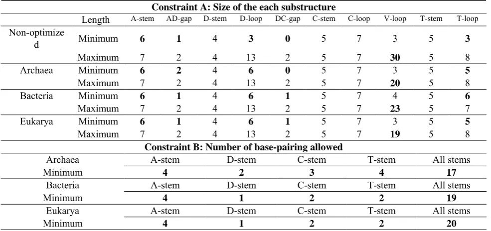
B.Result of Parameter Optimization for the tRNA Substructure and Each Base-pairing Allowed
Table II shows the optimized parameters for the size of each tRNA substructure and the number of each base-pairing allowed. In this section, we compare the non-optimized parameters and optimized parameters in Tables I and II. The
three species are described separately as follows:
(i). Archaea: Four stacked pairs - A-stem is 6 to 7 bp long, D-stem is 4 bp long, C-stem is 5 bp long, T-stem is 5 bp long. Four hairpin loops - T-loop is 5 to 8 bases long, V-loop is 3 to 20 bases long, C-loop is 7 bases long, and D-loop is 6 to 13 bases long. AD-gap is 2 bases long and DC-gap is 0 to 2. Minimum base-pairing achieved in each stem - A-stem is 4 bp, D-stem is 2 bp, C-stem is 3 bp, T-stem is 4 bp and All-stem is 17 bp.
(ii). Bacteria: Four stacked pairs - A-stem is 6 to 7 bp long, D-stem is 4 bp long, C-stem is 5 bp long, T-stem is 5 bp long. Four hairpin loops - T-loop is 6 to 7 bases long, V-loop is 4 to 23 bases long, C-loop is 7 bases long, and D-loop is 6 to 13 bases long. The AD-gap is 1 to 2 bases long and DC-gap is 1 to 2. Minimum base-pairing achieved in each stem - A-stem is 4 bp, D-stem is 1 bp, C-stem is 2 bp, T-stem is 2 bp, and All-stem is 19 bp.
[image:4.595.41.555.432.525.2](iii). Eukarya: Four stacked pairs - A-stem is 6 to 7 bp long, D-stem is 4 bp long, C-stem is 5 bp long, T-stem is 5 bp long. Four hairpin loops - T-loop is 5 to 8 bases long, V-loop is 3 to 19 bases long, C-loop is 7 bases long, and D-loop is 6 to 13 bases long. The AD-gap is 1 to 2 bases long and DC-gap is 1 to 2. Minimum base-pairing achieved in each stem - A-stem is 4 bp, D-stem is 1 bp, C-stem is 2 bp, T-stem is 2 bp, and All-stem is 20 bp.
TABLE I. Non-optimized constraints and parameters in the search of tRNA secondary structure. The loosest constraint A: Substructure length
A-stem AD-gap D-stem D-loop DC-gap C-stem C-loop V-loop T-stem T-loop
Default 6 to 7 2 4 4 to 11 1 5 7 4 to 21 5 4 to 7
Region 6 to 7 1 to 2 4 3 to 13 0 to 2 5 7 3 to 30 5 3 to 8
The loosest constraint B: Number of base-pairing achieved
A-stem D-stem C-stem T-stem All stems
Default 5 2 3 3 15
[image:4.595.53.546.551.783.2]Region 0 to 6 0 to 4 0 to 5 0 to 5 0 to 21
TABLE II. Optimized parameters and constraints. Constraint A: Size of the each substructure
Length A-stem AD-gap D-stem D-loop DC-gap C-stem C-loop V-loop T-stem T-loop
Non-optimize
d Minimum 6 1 4 3 0 5 7 3 5 3
Maximum 7 2 4 13 2 5 7 30 5 8
Archaea Minimum 6 2 4 6 0 5 7 3 5 5
Maximum 7 2 4 13 2 5 7 20 5 8
Bacteria Minimum 6 1 4 6 1 5 7 4 5 6
Maximum 7 2 4 13 2 5 7 23 5 7
Eukarya Minimum 6 1 4 6 1 5 7 3 5 5
Maximum 7 2 4 13 2 5 7 19 5 8
Constraint B: Number of base-pairing allowed
Archaea A-stem D-stem C-stem T-stem All stems
Minimum 4 2 3 4 17
Bacteria A-stem D-stem C-stem T-stem All stems
Minimum 4 1 2 2 19
Eukarya A-stem D-stem C-stem T-stem All stems
C.Comparison of optimized and non-optimized parameter performance efficiency
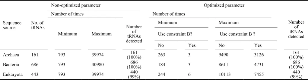
[image:5.595.310.548.68.189.2]The performance comparison of optimized and non-optimized parameters is shown in Table III, which is divided into two parts: results that do and do not use the optimized parameters for prediction of tRNA’s secondary structure. For the number of detected tRNAs, both the non-optimized parameter and the optimized parameters are the same, which indicates that all tRNA genes in the Sprinzl database are effectively predicted by this optimized parameter. Different inputting sequences require different search iterations. Hence, we used the minimum and the maximum numbers of times to demonstrate that the search time is effectively improved. Table III shows promising performance for search time in which the constraint B was used to demonstrate the considerable impact on its parameter. The substructure parameter optimization from Table II does not consider the constraint B. For the minimum number of times, the parameters optimized for the three species are 263, 184, and 244, respectively. For the maximum number of times, the optimized parameters for the three species are 9490, 8611, and 10113, respectively. Next, the constraint B was considered within the substructure parameter optimization from Table II. These numbers of times using the constraint B represent that the combination is satisfied with these constraints, i.e., A-stem, D-stem, C-stem, D-stem, and All-stem allowed. For the minimum number of times, the optimized parameters for the three species are 3, 3, and 6, respectively. For the maximum number of times, the optimized parameters for the three species are 3126, 4731, and 7455, respectively. Thus, the advantage of parameter optimization is clearly displayed with less time required than in the non-optimized situation.
Dynamics of logistic map
0 0.2 0.4 0.6 0.8 1
0 50 100 150 200 250 300
Number of Generations
C
hao
ti
c
Cr
va
lu
[image:5.595.42.553.643.777.2]e
Figure. 4 Chaotic Cr value using a logistic map for 300 iterations; Cr(0) = 0.001
D. Advantage of the Chaos algorithm
The standard PSO, together with each individual and the whole population, evolves towards best fitness in which the fitness function is evaluated with the objective function. Although this scheme has the property to increasing convergence capability (i.e., evolving the population toward better fitness), if the convergence speed is too fast, the population may get stuck in a local optimum since the swarms diversity rapidly decreases. On the other hand, the search speed cannot be set at an arbitrarily slow speed if we want PSO to be effective. The chaotic map is a very powerful tool for avoiding entrapment in local optima, and it does not increase complexity. The computational complexity for CPSO and PSO can be derived as O(PG), where P is the population size and G is the number of iterations. In Eq. 4, the chaotic map is only used to amend the PSO updating equation. Chaos is a non-linear system with ergodic, stochastic and regularity properties, and is very sensitive to its initial conditions and parameters. Consequently, CPSO is more efficient than the standard PSO because of the chaotic property, i.e., a small variation in an initial variable will result in a huge difference in the solutions after several iterations. Fig. 4 shows how the behavior of the chaos system for the logistic map is sensitive to initial conditions. Since logistic maps are frequently used as chaotic behavior maps and the chaotic sequences can be quickly generated and easily stored, there is no need to store long sequences [13].
Table III. Optimized and non-optimized parameter performance comparison.
Sequence
source No. of tRNAs
Non-optimized parameter Optimized parameter
Number of times Number of times
Minimum Maximum
Number of tRNAs detected
Minimum Maximum Number
of tRNAs detected
Use constraint B? Use constraint B ?
No Yes No Yes
Archaea 161 793 39974 (100%)161 263 3 9490 3126 161 (100%)
Bacteria 686 793 40980 (100%)686 184 3 8611 4731 686 (100%)
E.Analysis parameter optimized
The size of the substructures is improved in terms of the search time. During the search process, we noticed that an identical sequence appearing in several different configurations had the same anticodon. This unexpected finding brought our attention to the length of a secondary structure, which suggests that the correct anticodon may be folded through many of the substructures’ combinations and they are all able to satisfy the tRNA rules. Although many published methods use these common features to predict tRNA secondary structures, the substructures’ size from the known tRNA genes are the key to predicting the tRNA’s secondary structure. As seen in Table III, the tRNA characteristic relationship between the number of
times and the number of base-pairs achieved shows an unexpected result, i.e., of the three species, the Archaea has the lowest number of times at 3126. This should not be smaller than the number of times for bacteria because the archaea has to consider the intron structure, in which the archeae’s intron may be from 6 to 121 bases long, whereas bacteria have no introns. In analysis, the limits on the number of base-pairs is achieved is mainly by reducing required computation. The comparison between the bacteria and the eukaryota can also be observed.
F.Summary of contribution of this work to tRNA research field
In summary, the advantages of parameter optimization are as follows:
(i). Based on the tRNA cloverleaf model, this work provides a reliable prediction of tRNA secondary structure. The sizes of the substructures are optimized according to different species to increase the likelihood of detecting any tRNA genes.
(ii). Reliable limits for substructure base-pairing are provided to help tRNA research. Experimental results suggest the need for a deeper investigation when the predictions disagree with different tRNA search tools. For instance, an unknown tRNA gene was predicted by PtRNASS, but the result could be a false state. Hence, other computer programs, e.g., tRNAscan-SE [14], ARAGORN [15], were also used to enhance the completeness and accuracy of the prediction. These programs complement each other by either giving a secondary structure of tRNA identification when predicting the same result, or by suggesting a deeper investigation when the results disagree.
III. CONCLUSION
We have presented a computational method, based on Chaotic Particle Swarm Optimization, for optimizing the substructure and rule restriction allowed in three species. The experimental results demonstrate that this parameter can predict the correct anticodon and to reduce unnecessary computations in the tRNA secondary structure search process. In addition, the base-pairing limits the tRNA cloverleaf folding procedure, in which this parameter is
structure in the Sprinzl database. The results increase the analysis effectiveness of structural accuracy and anticodons from tRNA genes. We believe this work to be first use of artificial intelligence techniques for the task of tRNA parameter optimization, and it allows biologists and researchers to locate tRNA gene with greater efficiency.
REFERENCES
[1] J.R., Macey, J.A., 2nd, Schulte, A., Larson, B.S., Tuniyev, N. Orlov, and T.J. Papenfuss, “Molecular Phylogenetics, tRNA Evolution, and Historical Biogeography in Anguid Lizards and Related Taxonomic Families,” Molecular Phylogenetics and Evolution, Vol.12, No.3, 1999, pp. 250-272.
[2] F.J. Sun, and G. Caetano-Anolles, “Evolutionary patterns in the
sequence and structure of transfer RNA: early origins of archaea and viruses,” PLoS Comput Biol, 4, 2008, e1000018.
[3] M. Sprinzl, and K.S., Vassilenko, “Compilation of tRNA sequences
and sequences of tRNA genes,” Nucleic Acids Research, 33, 2005, pp.139-140.
[4] L.Y., Chuang, Y.D., Lin, and C.H., Yang, “PtRNASS: Prediction of
tRNA Secondary Structure from Nucleotide Sequences,” IAENG
International Journal of Computer Science, 37:3, IJCS_37_3_02,
2010, pp. 204-209.
[5] L.Y., Chuang, Y.D., Lin, and C.H., Yang, “A Method of Predicting
tRNA Secondary Structure from Nucleotide Sequences,” Lecture
Notes in Engineering and Computer Science: Proceedings of The International MultiConference of Engineers and Computer Scientists
2010, IMECS 2010, 17-19 March, 2010, Hong Kong, pp. 223-227. [6] J. Kennedy and R.C. Eberhart, “Particle swarm optimization,” IEEE
International Conference on Neural Networks, Perth, Australia, 1995,
Vol. 4, pp. 1942-1948.
[7] I. C. Trelea, “The particle swarm optimization algorithm: convergence analysis and parameter selection,” Information Processing Letters 85, 2003, pp. 317-325.
[8] S. Naka, T. Genji, T. Yura, Y. Fukuyama, “A hybrid particle swarm optimization for distribution state estimation,” IEEE Transactions on Power Systems 18, 2003, pp. 60-68.
[9] Y. Shi and R.C. Eberhart, “Empirical study of particle swarm
optimization,” Proceedings of Congress on Evolutionary
Computation, Washington, DC, 2002, pp. 1945-1949.
[10] H. G. Schuster, “Deterministic chaos: an introduction, 2nd revised ed.
Weinheim,” Federal Republic of Germany: Physick-Verlag GmnH,
1988.
[11] Z. Lu, L. S. Shieh, G. R. Chen, “On robust control of uncertain chaotic systems: a sliding-mode synthesis via chaotic optimization,” Chaos, Solitons & Fractals 18, 2003, pp. 819-827.
[12] Y. Shi and R.C. Eberhart, “A modified particle swarm optimizer,”
Proceedings of IEEE International Conference on Evolutionary Computation, Anchorage,” AK, May 1998, pp. 69-73.
[13] H. Gao, Y. Zhang, S. Liang, and D. Li, “A new chaotic algorithm for image encryption,” Chaos Solitons & Fractals, Vol. 29, Issue 2, July
2006, pp. 393-399.
[14] Lowe, T.M. and Eddy, S.R. “tRNAscan-SE: a program for improved
detection of transfer RNA genes in genomic sequence,” Nucleic Acids Research, Vol.25, 1997, pp.955-964.
[15] L. Dean and C. Bjorn, “ARAGORN, a program to detect tRNA genes