Abstract— A mathematical analysis is executed with respect to an end-of-period clearance pricing for daily perishable products. In case that supplied products will not be sold out by the end-of-period, the sales floor manager sometimes sells the products at a discount price in order to increase the revenue of the period. At a same time, the reference price of consumers for the products is consequently declined and some consumers would not purchase the products at a regular sales price in the following periods. It is important for the manager to take the reference price effect into account so as to improve long-term profit. This paper formulates the end-of-period inventory clearance problem for a single period with stochastic variations both on demand and on the inventory level at the end-of-period. The expected profit function depends on the consumer’s response against the sales price. A procedure is proposed to derive an optimal clearance price when consumers are loss-neutral. A sufficient condition is shown to simplify a similar procedure to obtain an optimal price for loss-averse and loss-seeking consumers.
Index Terms— clearance, inventory, optimal operation, reference price.
I. INTRODUCTION
Nowadays, a range of prepared foods, such as sushi, sliced raw fish, fried meals, cooked food, salad, are sold in retail stores in many countries. In case that the life of such products only lasts one day due to deterioration of freshness, firms prepare appropriate amount of the products before opening hour with predicting the demand of the day, and sell them just for the day. Unsold products are to be disposed or reused as ingredients for other products. The firms hope to reduce the number of unsold products from both economical and ecological standpoints. When the firms overestimate the demand, they sometimes discount the sales price of products or distribute coupons in order to stimulate consumer spending.
Such actions can improve profit of the day; they might increase the revenue and decrease disposal cost. At the same time, however, the action drops consumers' reference price for the product, with which consumers judge if a sale price is a gain or a loss. The declined reference price reduces the future demand for the products sold at a regular price, which is called the reference price effect on demand, and it might Manuscript received January 18, 2012. This work was partly supported by Grant-in-Aid for Scientific Research(C), 2011, No.22510147 and MEXT, Japan.
Takeshi Koide is with Department of Intelligence and Informatics, Konan University, Kobe 658-8501, Japan (corresponding author, e-mail: [email protected]).
Hiroaki Sandoh is with Department of Management Science and Business Administration, Graduate School of Economics, Osaka University, Toyonaka 560-0043, Japan (e-mail: [email protected])
decrease revenue in the long run. From a long-term business perspective, firms should discount sales prices advisedly.
The reference price is well-known as the reference point in the prospect theory proposed by Kahneman and Tversky [1]. There are some researches studying promotional planning problems with the reference price effect to derive optimal pricing policies to maximize long-term revenues [2, 3, 4]. They targeted frequently purchased commodities and implicitly assumed that the firm could procure enough amounts of products to satisfy demands. In their models, the discount aims to stimulate demand and not to decrease the disposals of unsold products. The inventory quantity of the products is neglected in their models. Petruzzi and Dada discussed the relationship between discount pricing and inventory control [5]. Their model derives both an optimal price and an optimal inventory level, but the reference price effect is not incorporated in their model.
This study analyzes an expected profit function mathematically to treat stochastic demand and inventory level in a single period model as a fundamental study for multi-period optimal pricings. As the results of the analysis, the profit function for loss-neutral consumers is proved to be concave and the optimal clearance price is derived through a first order condition. For loss-averse and loss-seeking consumers, the function could be concave or bimodal and the optimal prices are obtained by a procedure using first order conditions. A sufficient condition is derived to simplify the procedure when target consumers are loss-averse or loss-seeking.
II. BACKGROUNDS AND SETTINGS
A. Optimal Pricing and Inventory Level
Consider a price-setting firm which deals in a single type of perishable products. The firm cannot be sold the unsold products in the following periods. The firm determines the sales price p and the inventory level q to maximize the expected profit in a single period. The optimums p* and q* can be solved within a framework of the famous newsvendor problem [5].
Let D(p) = 0 – 1p + d be the stochastic demand
function with respect to p, where 0 , 1 > 0 and d is a
random variable with mean 0 and range [dL, dH]. When it
holds D(p)q, the q – D(p) products are unsold and be disposed or reused at the unit cost h, where h means the disposal cost if h > 0, and the salvage cost if h < 0. On the other hand, if it holds D(p) > q, the D(p) – q demands are not satisfied and estimated a penalty at the unit cost s > 0. Let c be the unit procurement cost of the products.
Introducing z = q – E[D(p)], so-called stocking factor, the optimal price p* which maximizes the expected profit Π , is given by the following equation [5]:
An Optimal Daily Inventory Clearance Operation
with Consumer’s Reference Price
1 0 * 2 ) ( z p
p , (1)
where (z) is the expected amounts of shortages and p0 is the optimal price which maximizes the riskless expected profit E[(p – c)D(p)]. From (1), the optimum p* only depends on z. With letting p = p*(z), the expected profit (p*(z), z) becomes just a function with respect to z, then the optimal stocking factor z* can be derived, then both p*
and q* are also derived [5].
B. Reference Price Effect
The demand function comprising the reference price effects is modeled as follows:
D(p, r) = 0 – 1p + 2G[r – p]+ – 2L[p – r]+, (2)
where 2G, 2L > 0 and [x]+ = max(x, 0). Consumers perceive
a sold product as a gain if the sales price p is less than their reference prices r, and the demand is increased by 2G(r – p)
from the fundamental demand D(p). If the sales price p is above the reference price r, the demand is decreased by 2L(p – r). When it holds 2G < 2L, 2G = 2L, and 2G > 2L,
the consumers are respectively referred as to loss-averse (LA), loss-neutral (LN), and loss-seeking (LS) [1].
The consumers update their reference prices depending on the sales price. It is assumed that the reference price rt on
period t + 1 is determined by the reference price rt + 1 and the
sales price pt on the previous period:
rt + 1 = rt + (1 – ) pt. (3)
The exponential smoothing represented by (3) is the most commonly adopted in the literature [2, 3, 4]. The smoothing parameter implies how strongly the reference price is affected by past prices, where 01. The consumers with lower have a short-term memory, and they are strongly influenced by recent sales prices. This study does not consider the reference price update since our target in this paper is an optimal operation on single period perishable products.
C. Problem Settings
At a prescheduled time during the operation hours, the store could discount the products to stimulate demand. This study focuses on the optimal discount pricing. The only decision variable in this model is the discount price p in the range [pL, pH], where pH means the regular price of the
products. The firm determines the price p before the prescheduled time with considering uncertain inventory level Q and consumer’s reference price r of the day for the products. If some products are unsold at the prescheduled time, the unsold products are sold at price p from then to closing time. The reference price r exists in the range [pL, pH]. The inventory level Q is assumed to be a random
variable and it is given by Q = q + q, where q is the average
of Q and q is a random factor whose mean is 0 and range is
[qL, qH]. Assume –h < c < pL and D(p, r) > 0 for any
, ∈ ,
III. OPTIMAL PRICING ANALYSIS
A. Optimal Pricing for LN Consumers
This subsection discusses the optimal pricing for LN consumers. Let , then the expected demand function d(p, r) = E[D(p, r)] is given by the following equation: . ) ( ) ( ) ,
(p r 0 1p 2 r p B0 r B1p
d (4)
The both parameters B0(r) and B1 are positive.
In accordance with Petruzzi and Dada [5], define new variables z = q – d(p, r) and = q – d. Note that
Q – D(p, r) = z + . (5)
The average of is 0 and the range of is , where and . Then, the profit (p, q, r) is expressed
, , , 0,
, . (6)
Let ∙ and ∙ be the probabilistic density function and the distribution function of the variable . Define
∙ 1 ∙ . The expected profit Π , , , hence, is obtained by
Π , , ,
+ . (7)
The expected profit (p, q, r) can be rewritten by
Π , , Ψ , , , (8)
Ψ , , , (9)
, Λ Θ , (10)
Λ , (11)
Θ . (12)
In (8), (p, r) and L(p, z) respectively imply the profit for
Q = D(p, r) and the expected cost incurred by excess or deficiency of inventory. The expected volumes of excess and deficiency of inventory are denoted by (z) and (z) defined in (11) and (12), respectively.
Differentiating from (8) to (12) with respect to p yields
, , (13)
Λ
, (14)
Θ
, (15)
,
Θ , (16)
Ψ ,
2 , (17)
, ,
2 Θ ,(18)
, ,
2 . (19)
Using the assumption of h < pL, Equations (18) and (19)
g(p, q, r) = B0(r) – (2p +h)B1 + (p + h + s)B1F(–z) – (–z).(20)
Hence, the following theorem has proved.
Theorem 1. When both the demand function D(p, r) and the inventory level Q are stochastic and consumers are LN, the expected profit (p, q, r) is concave with respect to p. The optimal price p*(q, r) which maximizes (p, q, r) is derived by the following equation:
∗ , min max ̂ , , ,
, (21)
where ̂ , is the unique solution of g(p, q, r)= 0:
Let ̅ be the 2 which satisfies ̂ , then ̅ is
obtained from the equation g(r, q, r) = 0:
̅ ,
, . (22)
Differentiating from Equations (8) to (12) with respect to 2
yields
, (23)
,
, (24)
Ψ ,
, (25)
, ,
2 , (26)
, ,
2 0. (27)
The expected profit Π , , is proved to be concave with respect to 2 from (27). When the following inequality holds
, , (28)
Equation (26) introduces that the expect profit Π , , is increasing, constant, and decreasing with respect to 2 for
p < r, p = r, and p > r, respectively. In other words, the maximum of Π , , is decreasing and increasing with respect to 2 for 2 < ̅ and 2 > ̅ , respectively. Hence, the
next lemma has proved.
Lemma 1. When both the demand function D(p, r) and the inventory level Q are stochastic and consumers are LN, the expected profit (p, q, r) is concave with respect to 2. Furthermore, in case that (28) holds, ̂ , is decreasing with respect to2.
B. Optimal Pricing for Asymmetric Consumers
For asymmetric LA and LS consumers, it holds . The expected profit function (p, q, r), hence, is expressed as
Π , , Π , , if ,
Π , , otherwise (29)
where G(p, q, r) and L(p, q, r) are respectively the profit
(p, q, r) with 2 = 2G and 2 = 2L. The two functions
G(p, q, r) and L(p, q, r) have a common point on p = r.
Let ̂ and ̂ be respectively the prices to maximize G(p, q, r) and L(p, q, r).
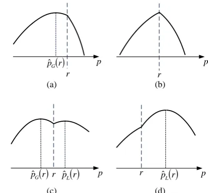
Lemma 1 restricts the possibility of the shape of the expected profit functions (p, q, r) for LA and LS consumers, represented in Fig. 1. The function (p, q, r) is concave except in the case of ̂ ̂
represented in Fig. 1(c), when the function is bimodal. This discussion introduces the following theorem as a procedure to derive the optimal price for the asymmetry consumers. Theorem 2. When both the demand function D(p, r) and the inventory level Q are stochastic and consumers are LA or LS, the optimal price p*(q, r) which maximizes the expected profit (p, q, r) is derived by the following equations:
∗
̂ , ̂
̂
̂
if ̂ ̂ ,
if max ̂ , ̂ , if min ̂ , ̂ , otherwise,
(30)
∗ min max , ̅ , , , | ∈ ∗ . (31) ∗ , argmax
∈ ∗ , , , (32)
Note that the cardinality of ∗ is two in the case of ̂ ̂ . In the other cases, the cardinality is one and (31) explores the optimal price without (32).
If (28) holds, the procedure given by Theorem 2 can be simplified. From lemma 2, it holds ̂ ̂ for LA consumers and ̂ ̂ for LS consumers. Hence, the following corollaries specific to LA and LS consumers are induced.
Corollary 1. When consumers are LA and (28) holds for p = pL, (30) can be replaced with the following equation:
∗
̂ if ̂ ,
if ̂ ̂ ,
̂ otherwise.
(33)
Corollary 2. When consumers are LS and (28) holds for p = pL, (30) can be replaced with the following equation:
∗
̂ if ̂ ,
̂ , ̂ if ̂ ̂ ,
̂ otherwise.
(34)
It is noticeable that (28) can be written as follows:
Pr , , (35)
r
p r
p
r pˆGr pˆL
r p
r pGˆ r pˆL
r p(a) (b)
[image:3.595.313.528.50.249.2](c) (d)
Fig. 1. The feasible shapes of the function (p, q, r). (a) ̂ and
̂ (b) ̂ and ̂ (c) ̂ ̂
(d) ̂ and ̂ .
IV. CONCLUSIONS
This study discussed a clearance pricing optimization in a single period analytically considering consumer’s reference price effect. The expected profit function is concave if target consumers are LN. For LA and LS consumers, the function is concave or bimodal. The optimal price for each type of consumers is derived through the procedures shown in Theorem 1. If (28) holds for p = pL, the
procedures can be simplified as shown in Corollaries 1 and 2.
The optimal prices are dependent on the consumer’s reference price r. The resulting properties with respect to the expected profit function are useful to derive an optimal clearance pricing in a multi-period case, which is the goal of our forthcoming study. The model in this paper can be modified to a combinatorial optimization. The resulting properties with respect to the expected profit function could serve to reduce computational time to explore the optimal solutions.
REFERENCES
[1] D. Kahneman and A. Tversky, “Prospect theory: An analysis of decision under risk,” Econometrica, vol. 47, 1979, pp. 263–291. [2] E. A. Greenleaf, “The impact of reference price effects on the
profitability of price promotions,” Marketing Science, vol. 14, 1995, pp. 82–104.
[3] P. K. Kopalle, A. G. Rao, and J. L. Assuncao, “Asymmetric reference price effects and dynamic pricing policies,” Marketing Science, vol. 15, 1996, pp. 60–85.
[4] I. Popescu and Y. Wu, “Dynamic pricing strategies with reference effects,” Operations Research, vol. 55, 2007, pp. 413–429.
[5] N. C. Petruzzi and M. Dada, “Pricing and the newsvendor problem: A review with extensions,” Operations Research, vol. 47, 1999, pp. 183–194.
[6] G. Kalyanaram and R. S. Winer, “Empirical generalizations from reference price and asymmetric price response research,” Marketing Science, vol. 14, pp. G161-G169, 1995.