Learning Algorithms for Stochastic Dynamic Pricing and Inventory Control.

(1)

Learning Algorithms for

Stochastic Dynamic Pricing and Inventory Control

by Boxiao Chen

A dissertation submitted in partial fulfillment of the requirements for the degree of

Doctor of Philosophy

(Industrial and Operations Engineering) in The University of Michigan

2016

Doctoral Committee:

Professor Xiuli Chao, Co-Chair Professor Hyun-Soo Ahn, Co-Chair Associate Professor Brian Denton Assistant Professor Cong Shi

(2)

c

(3)

ACKNOWLEDGEMENTS

First of all, I would like to thank my dissertation co-chairs Prof. Xiuli Chao and Prof. Hyun-Soo Ahn for their time and effort in guiding me through this Ph.D. journey. Without their support and help, this dissertation would not have been possible. One chapter in the dissertation also involves Prof. Cong Shi, from whom I have learned a lot. I would also like to thank my committee members Prof. Brian Denton and Prof. Xun Wu, for their helpful discussions and feedback.

My gratitude also goes to professors in the IOE department from whose lectures I have learned methodologies and techniques to conduct my research, including Prof. Marina Epelman, Prof. Jon Lee, Prof. Edwin Romeijn, Prof. Romesh Saigal and Prof. Robert Smith. And I also owe my thanks to staff members of the department for their assistance and help.

I appreciate the friendship from Prof. Xiuli Chao’s research group, which includes former members Dr. Xiting Gong, Dr. Jingchen Wu, Dr. Gregory King and Dr. Majid Al-Gwaiz, and current members Huanan Zhang, Sentao Miao and Duo Xu. Their feedback and comments help me a lot in my processes of doing researches and job hunting. I would also like to thank all my other friends for their caring and sharing.

Finally, I would like to thank my dearest parents for their unconditional love that carries my through many difficulties during my Ph.D. study. Their encouragement and support have always been the best source of energy to keep me moving forward, not only in pursuing my Ph.D., but also in life.

(4)

LIST OF FIGURES

Figure

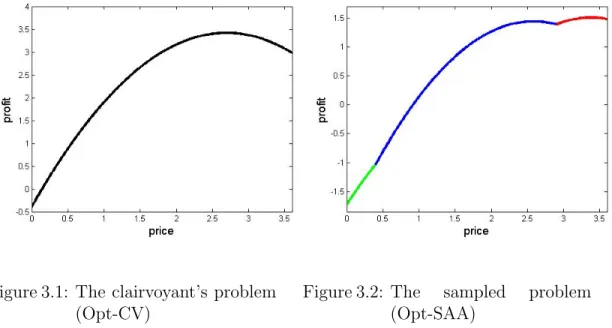
3.1 The clairvoyant’s problem (Opt-CV) . . . 73

3.2 The sampled problem (Opt-SAA) . . . 73

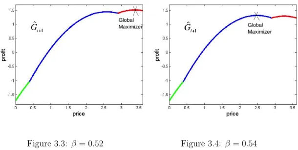
3.3 β = 0.52 . . . 99

3.4 β = 0.54 . . . 99

3.5 Sparse discretization and uniform closeness . . . 104

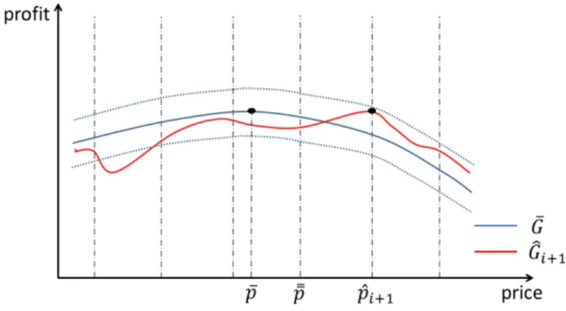
3.6 Choosing ¯p¯to be the closet point on the grid to ¯p, and also on the same side as ˆp(relative to ¯p) . . . 105

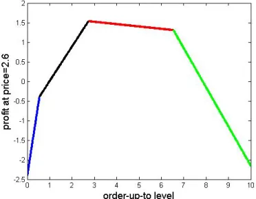
3.7 The sampled profit as a function of order-up-to level y (for a fixed price p= 2.6) in Example III.1 . . . 111

3.8 Choosing ¯p¯to be the closet point on the grid to ¯p, and also on the same side as ˆp(relative to ¯p) . . . 130

(7)

LIST OF TABLES

Table

2.1 Exponential Demand . . . 24

2.2 Logit Demand . . . 24

3.1 Percentage of Profit Loss (%) . . . 97

(8)

ABSTRACT

Learning Algorithms for Stochastic Dynamic Pricing and Inventory Control by

Boxiao Chen

Chair: Xiuli Chao, Hyun-Soo Ahn

This dissertation considers joint pricing and inventory control problems in which the customer’s response to selling price and the demand distribution are not known a priori, and the only available information for decision-making is the past sales data. Data-driven algorithms are developed and proved to converge to the true clairvoyant optimal policy had decision maker known the demand processes a priori, and, for the first time in literature, this dissertation provides theoretical results on the convergence rate of these data-driven algorithms.

Under this general framework, several problems are studied in different settings. Chapter 2 studies the classical joint pricing and inventory control problem with back-logged demand, and proposes a nonparametric data-driven algorithm that learns about the demand on the fly while making pricing and ordering decisions. The per-formance of the algorithm is measured by regret, which is the average profit loss compared with that of the clairvoyant optimal policy. It is proved that the regret vanishes at the fastest possible rate as the planning horizon increases.

(9)

First, due to demand censoring, the firm cannot observe either the realized demand or realized profit in case of a stockout, therefore only biased data is accessible; second, the data-driven objective function is always multimodal, which is hard to solve and establish convergence for. Chapter 3 presents a data-driven algorithm that actively explores in the inventory space to collect more demand data, and designs a sparse dis-cretization scheme to jointly learn and optimize the multimodal data-driven objective. The algorithm is shown to be very computationally efficient.

Chapter 4 considers a constraint that only allows the firm to change prices no more than a certain number of times, and explores the impact of number of price changes on the quality of demand learning. In the data-driven algorithm, we extend the traditional maximum likelihood estimation method to work with censored demand data, and prove that the algorithm converges at the best possible rate for any data-driven algorithms.

(10)

CHAPTER I

Introduction

Firms often integrate inventory and pricing decisions to match demand with sup-ply. For instance, a firm may offer a discounted price when there is excess inventory or raise the price when the inventory level is low. Since the seminal paper of Whitin (1955), the joint pricing and inventory control problems have attracted significant attention in the field (see, e.g., the survey papers by Petruzzi and Dada (1999), El-maghraby and Keskinocak (2003), Yano and Gilbert (2003), Chen and Simchi-Levi (2012)). Almost all papers on this topic assume that the firm knows how the market responds to its selling prices and the exact distribution of uncertainty in customer demand, and the inventory and pricing decisions are made with full knowledge of the underlying demand process. However, in practice, the demand-price relationship is usually not known a priori. Indeed, even with past observed demand data (often censored in the lost-sales case), it remains difficult to select the most appropriate functional form and estimate the distribution of demand uncertainty (see Huh and Rusmevichientong (2009), Huh et al. (2011), Besbes and Muharremoglu (2013), Shi et al. (2015) for more discussions on censored demand in various other inventory systems).

In Chapter 2, we consider a firm (e.g., retailer) selling a single nonperishable prod-uct over a finite-period planning horizon. Demand in each period is stochastic and

(11)

price-dependent, and unsatisfied demands are backlogged. At the beginning of each period, the firm determines its selling price and inventory replenishment quantity, but it knows neither the form of demand dependency on selling price nor the distribution of demand uncertainty a priori, hence it has to make pricing and ordering decisions based on historical demand data. We propose a nonparametric data-driven policy that learns about the demand on the fly and, concurrently, applies learned informa-tion to determine replenishment and pricing decisions. The policy integrates learning and action in a sense that the firm actively experiments on pricing and inventory levels to collect demand information with the least possible profit loss. Besides con-vergence of optimal policies, we show that the regret, defined as the average profit loss compared with that of the clairvoyant optimal solution when the firm had complete information about the underlying demand, vanishes at the fastest possible rate as the planning horizon increases.

In Chapter 3, we consider the classical joint pricing and inventory control prob-lem with lost-sales and censored demand in which the customer’s response to selling price and the demand distribution are not known a priori, and the only available information for decision-making is the past sales data. Conventional approaches, such as stochastic approximation, online convex optimization, and continuum-armed bandit algorithms, cannot be employed since neither the realized values of the profit function nor its derivatives are known. A major difficulty of this problem lies in the fact that the estimated profit function from observed sales data is multimodal even when the expected profit function is concave. We develop a nonparametric data-driven algorithm that actively integrates exploration and exploitation through carefully designed cycles. The algorithm searches the decision space through a sparse discretization scheme to jointly learn and optimize a multimodal (sampled) profit function, and corrects the estimation biases caused by demand censoring. We show that the algorithm converges to the clairvoyant optimal policy as the planning

(12)

hori-zon increases, and obtain the convergence rate of regret. Numerical experiments show that the proposed algorithm performs very well.

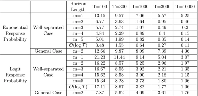
In Chapter 4, we consider a firm selling a product over T periods. Demand in each period is random and price sensitive, and unsatisfied demands are lost and unob-servable. The firm has limited prior knowledge about the demand process and needs to learn it through historical sales data. We consider the scenario where the firm is faced with the business constraint that prevents it from conducting extensive price experimentation. We develop data-driven algorithms for pricing and inventory deci-sions and evaluate their effectiveness using regret, which is the profit loss compared to a clairvoyant who has complete information about the demand process. We study three distinct scenarios and design algorithms that achieve the lowest possible regret rates: First, in a quite general case, when the number of price changes is bounded by a given number, the regret is O(T1/2_{). Second, in a special so-called well-separated}

case, when the number of price changes is limited to m, the regret is O(T1/m+1_).

Third, in the well-separated case allowing more frequent price changes that is limited to O(logT), the regret is O(logT). Numerical results show that these algorithms empirically perform very well.

(13)

CHAPTER II

Coordinating Pricing

and Inventory Replenishment

with Nonparametric Demand Learning

2.1 Introduction

Balancing supply and demand is a challenge for all firms, and failure to do so can directly affect the bottom-line of a company. From the supply side, firms can use operational levers such as production and inventory decisions to adjust inven-tory level in pace of uncertain demand. From the demand side, firms can deploy marketing levers such as pricing and promotional decisions to shape the demand to better allocate the limited (or excess) inventory in the most profitable way. With the increasing availability of demand data and new technologies, e.g., electronic data interchange, point of sale devices, click stream data etc., deploying both operational and marketing levers simultaneously is now possible. Indeed, both academics and practitioners have recognized that substantial benefits can be obtained from coordi-nating operational and pricing decisions. As a result, the research literature on joint pricing and inventory decisions has rapidly grown in recent years, see, e.g., the survey papers by Petruzzi and Dada (1999), Elmaghraby and Keskinocak (2003), Yano and

(14)

Despite the voluminous literature, the majority of the papers on joint optimization of pricing and inventory control have assumed that the firm knows how the market responds to its selling prices and the exact distribution of uncertainty in customer demand for any given price. This is not true in many applications, particularly with demand of new products. In such settings, the firm needs to learn about demand information during the dynamic decision making process and simultaneously tries to maximize its profit.

In this chapter, we consider a firm selling a nonperishable product over a finite-period planning horizon in a make-to-stock setting that allows backlogs. In each period, the firm sets its price and inventory level in anticipation of price-sensitive and uncertain demand. If the firm had complete information about the underlying demand distribution, this problem has been studied by, e.g.,Federgruen and Heching (1999), among others. The point of departure this paper takes is that the firm possesses limited or even no prior knowledge about customer demand such as its dependency on selling price or the distribution of uncertainty in demand fluctuation. We develop a nonparametric data-driven algorithm that learns the demand-price relationship and the random error distribution on the fly. We also establish the convergence rate of the regret, defined as the average profit loss per period of time compared with that of the optimal solution had the firm known the random demand information, and that is fastest possible for any learning algorithm. This work is the first to present a nonparametric data-driven algorithm for the classic joint pricing and inventory control problem that not only shows the convergence of the proposed policies but also the convergence rate for regret.

2.1.1 Literature Review

Almost all early papers in joint pricing and inventory control, e.g.,Whitin (1955), Federgruen and Heching (1999), and Chen and Simchi-Levi (2004a), among others,

(15)

assume that a firm has complete knowledge about the distribution of underlying stochastic demand for any given selling price. The complete information assumption provides analytic tractability necessary for characterizing the optimal policy. The extension to the parametric case (the firm knows the class of distribution but not the parameters) has been studied by, for example, Subrahmanyan and Shoemaker (1996), Petruzzi and Dada (2002), and Zhang and Chen (2006). Chung et al. (2011) also consider the problem of dynamic pricing and inventory planning with demand learning, and they develop learning algorithms using Bayesian method and Markov chain Monte Carlo (MCMC) algorithms, and numerically evaluate the importance of dynamic pricing. An alternative to the parametric approach is to model the firm’s problem in a nonparametric setting. Under this framework, the firm does not make specific assumptions about underlying demand. Instead, the firm makes decisions solely based on the collected demand data, seeBurnetas and Smith (2000). Our work falls into this category.

To our best knowledge,Burnetas and Smith(2000) is the only paper that considers the joint pricing and inventory control problem in a nonparametric setting. The authors consider a make-to-stock system for a perishable product with lost sales and linear costs, and propose an adaptive policy to maximize average profit. They assume that the price is chosen from a finite set and formulate the pricing problem as a multi-armed bandit problem, and show that the average profit under their approximation policy converges in probability. No convergence rate or performance bound is obtained for their algorithm.

Other approaches in the literature on developing nonparametric data-driven algo-rithms include online convex optimization (Agarwal et al. (2011), Zinkevich (2003), Hazan et al.(2007)), continuum-armed bandit problems (Auer et al.(2007),Kleinberg (2005), Cope (2009)), and stochastic approximation (Kiefer and Wolfowitz (1952b), Lai and Robbins (1981), and Robbins and Monro (1951)). In fact, Burnetas and

(16)

Smith (2000) is an example of implementing such algorithms to the joint pricing and inventory control problem. However, these methodologies require that the pro-posed solution be reachable in each and every period, which is not the case with our problem. This is because, in a demand learning algorithm of joint pricing/inventory control problem, in each period the algorithm utilizes the past demand data to pre-scribe a pricing decision and an order up-to level. However, if the starting inventory level of the period is already higher than the prescribed order up-to level, then the prescribed inventory level for the period cannot be reached. Actually, that is pre-cisely the reason that Burnetas and Smith (2000) focused on the case of perishable product (hence the firm has no carry-over inventory and the inventory decision ob-tained by Burnetas and Smith (2000) based on multi-armed bandit process can be implemented in each period). Agarwal et al. (2011),Auer et al.(2007), andKleinberg (2005) propose learning algorithms and obtain regrets that are not as good as ours in this chapter. Zinkevich (2003) and Hazan et al. (2007) present machine learning algorithms in which the the exact gradient of the unknown objective function at the current decision can be computed, and their results have been applied to dynamic inventory control inHuh and Rusmevichientong (2009). However, in the joint pricing and inventory control problem with unknown demand response, the gradient of the unknown objective function cannot be obtained thus the method cannot be applied.

2.1.2 Contributions and Comparison with Closely Related Literature

The closest related research works to ours are Besbes and Zeevi (2015),Levi et al. (2007) and Levi et al. (2011), offering nonparametric approaches to pure pricing problem (with no inventory) and pure inventory control problem (with no pricing), respectively.

Besbes and Zeevi (2015) consider a dynamic pricing problem in which a firm chooses its selling price to maximize expected revenue. The firm does not know

(17)

the deterministic demand curve (i.e., how the average demand changes in price) and learns it through noisy demand realizations, and the authors establish the sufficiency of linear approximations in maximizing revenue. They assume that the firm has infinite supply of inventory, or, alternatively, the seller has no inventory constraint. In this case, since the expected revenue in each period depends only on its mean demand, the distribution of random error is immaterial in their learning algorithm and analysis. On the other hand, in the dynamic newsvendor problem considered in Levi et al. (2007, 2010), the essence for effective inventory management is to strike a balance between overage cost and underage cost, for which the distribution of uncertain demand plays a key role. Levi et al. (2007) and Levi et al. (2011) apply Sample Average Approximation (SAA) to estimate the demand distribution and average cost function, and they analyze the relationship between sample sizes and accuracy of estimations and inventory decisions.

Our problem has both dynamic pricing and inventory control, and the firm knows neither the relationship between demand and selling price nor the distribution of demand uncertainty. In Besbes and Zeevi (2015), the authors only need to estimate the average demand curve in order to maximize revenue, and demand distribution information is irrelevant. In a remark, Besbes and Zeevi (2015) state that their method of learning the demand curve can be applied to maximizing more general forms of objective functions beyond the expected revenue which, however, does not apply to our setting. This is because, in the general form presented inBesbes and Zeevi (2015), the objective function still has to be a known function in terms of price and the demand curve for a given price and a given demand curve. Thus the firm must know the exact expression of the objective function when the estimate of a demand curve is given. In our problem, even with a given price and inventory level and a given demand curve, the objective function cannot be written as a known deterministic function. Indeed, this function contains the expected inventory holding and backorder costs

(18)

that depend on the distribution of demand fluctuation, which is also unknown to the firm. In fact, the latter is a major technical challenge encountered in this chapter because, as we will explain below, the estimation of the demand uncertainty, therefore also of the expected holding/shortage cost, cannot be decoupled with the estimation of the average demand curve, which is gathered through price experimentation.

Standard SAA method is implemented to the newsvendor problem by Levi et al. (2007) and Levi et al. (2011) which, however, cannot be applied to our setting for determining inventory decisions. InLevi et al.(2007) andLevi et al.(2011), dynamic inventory control is studied in which pricing is not a decision and it is assumed (implic-itly) to be given. The only information the firm is uncertain about is the distribution of random fluctuation. Therefore, the firm can observe true realizations of demand fluctuation which are used to build an empirical distribution. In our model, however, the firm knows neither how average demand responds to the selling price (demand curve) nor the distribution of fluctuating demand, but both of them affect demand re-alizations. For any estimation of average demand curve, the error of this estimate will affect the estimation of distribution of random demand fluctuation. Hence, through the realization of random demand we are unable to obtain a true realization of ran-dom demand error without knowing the exact average demand function. As a result, the standard SAA analysis is not applicable in our setting because unbiased samples of the random error cannot be obtained.

Because the firm does not know the exact demand curve a priori, its estimate of error distribution using demand data is inevitably biased, and as a result, the data-driven optimization problem constructed to compute the pricing and ordering strategies is also biased. Because of this bias, it is no longer true that the solution of the data-driven problem using SAA must converge to the true optimal solution. Fortunately, we are able to show that as the learning algorithm proceeds, the biases will be gradually diminishing and that allows us to prove that our learning algorithm

(19)

still converges to the true optimal solution. This is done by establishing several important properties of the newsvendor problem that bound the errors of biased samples. One main contribution of this chapter is to explicitly prove that the solution obtained from a biased data-driven optimization problem still converges to the true optimal solution.

Finally, we highlight on the result of the convergence rate of regret. Besbes and Zeevi (2015) obtain a convergence rate of T−1/2(logT)2 for their dynamic pricing problem, whereT is the length of the planning horizon. For the pure dynamic inven-tory control problem, Huh and Rusmevichientong (2009) present a machine learning algorithm with convergence rate T−1/2_{. For the joint pricing and inventory problem,}

we show that the regret of our learning algorithm converges to zero at rate T−1/2_,

which is also the theoretical lower bound. Thus, this chapter strengthens and extends the existing work by achieving the tightest convergence rate for the problem with joint pricing and inventory control. One important implication of our finding is that the linear demand approximation scheme ofBesbes and Zeevi (2015) actually achieves the best possible convergence rate of regret, which further improves the result of Besbes and Zeevi (2015). That is, nothing is lost in the learning algorithm in approximating the demand curve by a linear model.

2.1.3 Organization

The rest of this chapter is organized as follows. Section 2.2 formulates the problem and describes the data-driven learning algorithm for pricing and inventory control decisions. The following two sections (Sections 3 and 4) present our major theoretical results together with a numerical study, and the main steps of the technical proofs, respectively. The chapter concludes with a few remarks in Section 5. Finally, the details of the mathematical proofs are given in the Appendix.

(20)

2.2 Formulation and Learning Algorithm

We consider an inventory system in which a firm (e.g., a retailer) sells a nonper-ishable product over a planning horizon ofT periods. At the beginning of each period t, the firm makes a replenishment decision, denoted by the order-up-to level,yt, and a pricing decision, denoted by pt, where yt ∈ Y = [yl, yh] andpt∈ P = [pl, ph] for some known lower and upper bounds of inventory level and selling price, respectively. We assume ph _{> p}l _{since otherwise, the problem is the pure inventory control problem} and learning algorithms have been developed in Huh and Rusmevichientong (2009), Levi et al.(2007), andLevi et al.(2011). During periodtand when the selling price is set to pt, a random demand, denoted by ˜Dt(pt), is realized and fulfilled from on-hand inventory. Any leftover inventory is carried over to the next period, and in case the demand exceeds yt, the unsatisfied demand is backlogged. The replenishment lead-time is zero, i.e., an order placed at the beginning of a period can be used to satisfy demand in the same period. Let h and b be the unit holding and backlog costs per period, and the unit purchasing cost is assumed, without loss of generality, to be zero. The model as described above is the well-known joint inventory and pricing deci-sion problem studied in Federgruen and Heching (1999), in which it is assumed that the firm has complete information about the distribution of ˜Dt(pt). In this chapter we consider a setting where the firm does not have prior knowledge about the demand distribution.

In general, the demand in periodtis a function of selling priceptin that period and some random variable ˜t, and it is stochastically decreasing in pt. The most popular demand models in the literature are the additive demand model ˜Dt(pt) = ˜λ(pt) + ˜t and multiplicative demand model ˜Dt(pt) = ˜λ(pt) ˜t, where ˜λ(·) is a strictly decreas-ing deterministic function and ˜t, t = 1,2, . . . , T, are independent and identically distributed random variables. In this chapter, we shall study both additive and the

(21)

nor the distribution function of random variable ˜t. The firm has to learn from his-torical demand data, that are the realizations of market responses to offered prices, and use that information as a basis for decision making. Suppose ˜thas finite support [l, u], with l ≥0 for the case of multiplicative demand.

To define the firm’s problem, we letxt denote the inventory level at the beginning of period t before replenishment decision. We assume that the system is initially empty, i.e., x1 = 0. The system dynamics are xt+1 =yt−Dt(pt) for all˜ t= 1, . . . , T.

An admissible policy is represented by a sequence of prices and order-up-to levels, {(pt, yt), t ≥1}, where (pt, yt) depends only on realized demand and decisions made prior to period t, and yt ≥ xt, i.e., (pt, yt) is adapted to the filtration generated by {(ps, ys),D˜s(ps);s= 1, . . . , t−1}. The firm’s objective is to find an admissible policy to maximize its total profit.

If both the function of ˜λ(·) and the distribution of ˜t are known a priori to the firm (complete information scenario), then the optimization problem the firm wishes to solve is max (pt, yt)∈ P × Y yt≥xt T X t=1 ptE[ ˜Dt(pt)]−hE[yt−D˜t(pt)]+−bE[ ˜Dt(pt)−yt]+ , (2.1)

where_Estands for mathematical expectation with respect to random demand ˜Dt(pt), and x+ _{= max{x,}_0} _{for any real number} _{x. However, since in our setting the firm}

does not know the demand distribution, the firm is unable to evaluate the objective function of this optimization problem.

We develop a data-driven learning algorithm to compute the inventory control and pricing policy. It will be shown in Section 3 that the average profit of the algorithm converges to that of the case when complete demand distribution information is known a priori, and that the pricing and inventory control parameters also converge to that of the optimal control policy for the case with complete information as the

(22)

planning horizon becomes long. To save space we shall only present the algorithm and analytical results for the multiplicative demand model. The results and analyses for the additive demand case are analogous, and we only highlight the main differences at the end of this section.

Remark 1. For ease of exposition, in this chapter we assume the support of

un-certainty ˜t is bounded. This can be relaxed, and all the results hold as long as we assume the moment generating functions of the relevant random variables are finite in a small neighborhood of 0, or light tailed.

Case of complete information about demand. In the case of complete

infor-mation in which the firm knows ˜λ(·) and the distribution of ˜t, it follows from (2.1) that, if (p∗, y∗) is the optimal solution of each individual term

max p∈P,y∈Y n p_E[ ˜Dt(p)]−h_E[y−Dt(p)]˜ +−b_E[ ˜Dt(p)−y]+ o . (2.2)

and that this solution is reachable in every period, i.e., xt≤y∗ for all t, then (p∗, y∗) is the optimal policy for each period. We refer to p∗ and y∗ as the optimal price and optimal order up-to level (or optimal base-stock level), respectively. It is clear that the reachability condition is satisfied if the system is initially empty, which we assume.

We find it convenient to analyze (2.2) using a slightly different but equivalent form. Taking logarithm on both sides of ˜Dt(pt) = ˜λ(pt)˜t, we obtain

log ˜Dt(pt) = log ˜λ(pt) + log ˜t, t = 1, . . . , T.

Denote Dt(pt) = log ˜Dt(pt), λ(pt) = log ˜λ(pt) and t = log ˜t. Then, the logarithm of demand can be written as

(23)

We shall refer to λ(·) as the demand-price function (or demand-price curve) and t as random error (or random shock). Clearly, λ(·) is also strictly decreasing in p ∈ P. Hence, in the case of complete information, the firm knows the function λ(·) and the distribution of t, and when the firm does not know function λ(·) and the distribution of t, which is our case, the firm will need to learn about them. Without loss of generality, we assume_E[t] =E[log ˜t] = 0. If this is not the case, i.e., E[log ˜t] = a 6= 0, then E[log(e−αt)] = 0, thus if we let ˆ˜ λ(·) = eaλ(·) and ˆ˜ t =e−a˜t, then ˜Dt(pt) = ˆλ(pt)ˆt, and ˆλ(·) and ˆt satisfy the desired properties.

For convenience, letbe a random variable distributed as1. In terms ofλ(·) and

, we define

G(p, y) = peλ(p)_Ee−nh_Ey−eλ(p)e++b_Eeλ(p)e−y+o. Then problem (2.2) can be re-written as

Problem CI: max

p∈P,y∈YG(p, y) (2.4) = max p∈P n peλ(p)_Ee−min y∈Y n h_Ey−eλ(p)e++b_Eeλ(p)e−y+o o. The inner optimization problem (minimization) determines the optimal order-up-to level that minimizes the expected inventory and backlog cost for given pricep, and we denote it byy eλ(p)

. The outer optimization solves for the optimal price p. Let the optimal solution for (2.4) be denoted by p∗ and y∗, then they satisfy y∗ =y(eλ(p∗)_).

The analysis above stipulates that the firm knows the demand-price curve λ(p) and the distribution of , thus we refer to it as problem CI (complete information).

Learning algorithm. In the absence of the prior knowledge about the demand

process, the firm needs to collect the demand information necessary to estimateλ(p) and the empirical distribution of random error , thus price and inventory decisions

(24)

ficulty lies in that, the estimations of demand-price curve λ(p) and the distribution of random error cannot be decoupled. This is because, the firm only observes real-ized demands, hence with any estimation of demand-price curve, the estimation error transfers to the estimation of the random error distribution. Indeed, we are not even able to obtain unbiased samples of the random error t.

In our algorithm below we approximate λ(p) by an affine function, and construct an empirical (but biased) error distribution using the collected data. We divide the planning horizon into stages whose lengths are exponentially increasing (in the stage index). At the start of each stage, the firm sets two pairs of prices and order-up-to levels based on its current linear estimation of demand-price curve and (biased) empirical distribution of random error, and the collected demand data from this stage are used to update the linear estimation of demand-price curve and the biased empirical distribution of random error. These are then utilized to find the pricing and inventory decision for the next stage.

The algorithm requires some input parameters v, ρ and I0, with v > 1, I0 > 0,

and 0< ρ≤2−3/4_(ph₋_pl_)I1/4

0 . To initiate the algorithm, it sets {ˆp1,yˆ11,yˆ12}, where

ˆ

p1 ∈ P,yˆ11 ∈ Y,yˆ12 ∈ Y are the starting pricing and order-up-to levels. For i≥1, let

Ii =bI0vic, δi =ρ(2Ii−1)− 1 4, and t i = i−1 X k=1 2Ik with t1 = 0, (2.5)

where bI0vic is the largest integer less than or equal to I0vi.

The following is the detailed procedure of the algorithm. Recall that xt is the starting inventory level at the beginning of period t, pt is the selling price set for period t, and yt (≥ xt) is the order-up-to inventory level for period t, t = 1, . . . , T. The number of learning stages is n = llog_v₂v_I−1

0vT + 1

m

, where dxe denotes the smallest integer greater than or equal to x.

(25)

Step 0. Initialization. Choose v > 1, ρ > 0 and I0 > 0, and ˆp1,yˆ11,yˆ12.

Compute I1 =bI0vc, δ1 =ρ(2I0)−

1

4, and ˆp₁+δ₁.

Step 1. Setting prices and order-up-to levels for stage i. Fori= 1, . . . , n, set prices pt, t=ti+ 1, . . . , ti + 2Ii, to

pt= ˆpi, t=ti+ 1, . . . , ti+Ii,

pt= ˆpi+δi, t=ti+Ii+ 1, . . . , ti+ 2Ii;

and for t=ti+ 1, . . . , ti+ 2Ii, raise the inventory levels to

yt = max{ˆyi1, xt}, t=ti+ 1, . . . , ti+Ii, yt = max{ˆyi2, xt}, t=ti+Ii+ 1, . . . , ti+ 2Ii.

Step 2. Estimating the demand-price function and random errors us-ing data from stage i. Let Dt = log ˜Dt(pt) be the logarithm of demand realizations fort =ti+ 1, . . . , ti+ 2Ii, and compute

( ˆαi+1,βˆi+1) = argmin α,β ti+2Ii X t=ti+1 Dt−(α−βpt) 2 , (2.6)

ηt=Dt−( ˆαi+1−βiˆ+1pt), for t=ti+ 1, . . . , ti+ 2Ii. (2.7)

Step 3. Defining and maximizing the proxy profit function, denoted by

GDD_i₊₁(p, y). Define GDD_i₊₁(p, y) =peαî+1−βî+1p 1 2Ii ti+2Ii X t=ti+1 eηt ₋ 1 2Ii ti+2Ii X t=ti+1 hy−eαî+1−βî+1p_eηt + +beαî+1−βî+1p_eηt ₋_y + .

(26)

Then the data-driven optimization is defined by Problem DD: max (p,y)∈P×YG DD i+1(p, y) (2.8) = max p∈P peαî+1−βî+1p 1 2Ii ti+2Ii X t=ti+1 eηt −min y∈Y 1 2Ii ti+2Ii X t=ti+1 hy−eαî+1−βî+1p_eηt + +beαî+1−βî+1p_eηt₋_y + .

Solve problem DD and set the first pair of price and inventory level to

(ˆpi+1,yˆi+1,1) = arg max (p,y)∈P×YG

DD i+1(p, y),

and set the second price to ˆpi+1+δi+1 and the second order-up-to level to

ˆ

yi+1,2 = arg max

y∈Y G

DD

i+1(ˆpi+1+δi+1, y).

In case ˆpi+1+δi+1 6∈ P, set the second price to ˆpi+1−δi+1.

Remark 2. When ˆβi+1 > 0, the objective function in (2.8) after minimizing over

y ∈ Y is unimodal in p. To see why this is true, let d = eαˆi+1−βˆi+1p _{and thus}

p = αˆi+1−logd

ˆ

βi+1 with d ∈ D = [d

l_{, d}h_{], where} _dl ₌ _eαî+1−βî+1ph _and _dh ₌ _eαî+1−βî+1pl_.

Then the optimization problem (2.8) is equivalent to

max d∈D ( dαˆi+1−logd ˆ βi+1 1 2Ii ti+2Ii X t=t1+1 eηt ! −min y∈Y ( 1 2Ii ti+2Ii X t=ti+1 h(y−deηt₎+₊_b(deηt ₋_y)+ )) .

The objective function of this optimization problem is jointly concave in (y, d) hence it is concave in d after minimizing over y∈ Y. Thus, it follows from p= αˆi+1−logd

ˆ

βi+1 is

(27)

Remark 3. In Step 3 of DDA, the second price is set to ˆpi+1−δi+1 when ˆpi+1+δi+1 >

ph_{. In this case our condition} _ρ _≤ ₂−3/4_(ph ₋_pl_)I1/4

0 ensures that ˆpi+1−δi+1 ≥ pl,

thus ˆpi+1−δi+1 ∈ P.This is because, when ˆpi+1 > ph−δi+1, we have

ˆ

pi+1−δi+1> ph−2δi+1 ≥ph −2δ1 =ph−2ρ(2I0)−1/4 ≥pl,

where the last inequality follows from the condition onρ.

Discussion of algorithm and its connections with the literature. In our

algorithm above, iteration ifocuses on stagei that consists of 2Ii periods. In Step 1, the algorithm sets the ordering quantity and selling price for each period in stage i, and they are derived from the previous iteration. In Step 2, the algorithm uses the realized demand data and least-squares method to update the linear approximation,

ˆ

αi+1 −βˆi+1p, of λ(p) and computes a biased sample ηt of random error t, for t = ti+ 1, . . . , ti+ 2Ii. Note thatηtis not a sample of the random errort. This is because t = Dt(pt)−λ(pt) and the (logarithm of) observed demand is Dt(pt). However as we do not know λ(p), it is approximated by ˆαi+1−βˆi+1p, therefore

ηt =Dt(pt)−( ˆαi+1−βiˆ+1pt)6=Dt(pt)−λ(pt) =t.

For the same reason, the constructed objective function for holding and shortage costs is not a sample average of the newsvendor problem.

In the traditional SAA, mathematical expectations are replaced by sample means, see e.g., Kleywegt et al. (2002). Levi et al. (2007) and Levi et al. (2011) apply SAA method in dynamic newsvendor problems. The argument above shows that the tra-ditional analyses that show SAA leads to the optimal solution is not applicable to our setting. Indeed, in our inner layer optimization, we face a newsvendor problem for which the firm needs to balance holding and shortage cost, and the knowledge about demand distribution is critical. However, the lack of samples of random error

(28)

t makes the inner loop optimization problem significantly different from Levi et al. (2007) and Levi et al. (2011), which consider pure inventory control problems and samples of random errors are available for applications of SAA result and analysis. Because of this, it is not guaranteed that the SAA method will lead to a true optimal solution.

The DDA algorithm integrates a process of earning (exploitation) and learning (exploration) in each stage. The earning phase consists of the firstIi periods starting at ti+ 1, during which the algorithm implements the optimal strategy for the proxy problemGDD

i (p, y). In the nextIiperiods of learning phase that starts fromti+Ii+1, the algorithm uses a different price ˆpi +δi and its corresponding order-up-to level. The purpose of this phase is to allow the firm to obtain demand data to estimate the rate of change of the demand with respect to the selling price. Note that, even though the firm deviates from the optimal strategy of the proxy problem in the second phase, the policies, (ˆpi+δi,yˆi,2) and (ˆpi,yˆi,1), will be very close to each other asδi diminishes to zero. We will show that they both converge to the true optimal solution and the loss of profit from this deviation converges to zero.

The pricing part of our algorithm is similar to the pure pricing problem considered by Besbes and Zeevi (2015) as we also use linear approximation to estimate the demand-price function then maximize the resulting proxy profit function. Although our algorithm is heavily influenced by their work, there is a key difference. Besbes and Zeevi (2015) consider a revenue management problem and they only need to estimate the deterministic demand-price function, and the distribution of random errors is immaterial in their analysis. In our model, however, due to the holding and backlogging costs, the distribution of the random error is critical and that has to be learned during the decision process, but it cannot be separated from the estimation of demand-price curve, as discussed above.

(29)

learn-ing of demand-price curve and the random error distribution cannot be decoupld, we are not able to prove that the DDA algorithm converges to the true optimal solution by using the approaches developed inBesbes and Zeevi (2015) for the pricing problem and in Levi et al. (2007) for the newsvendor problem. To overcome this difficulty, we construct several intermediate bridging problems between the data-driven problem and the complete information problem, and perform a series of convergence analyses to establish the main results.

Performance Metrics. To measure the performance of a policy, we use two

metrics proposed in Besbes and Zeevi (2015): consistency and regret. An admissible policy π = ((pt, yt), t ≥1) is said to be consistent if (pt, yt) →(p∗, y∗) in probability as t → ∞. The average (per-period) regret of a policy π, denoted by R(π, T), is defined as the average profit loss per period, given by

R(π, T) =G(p∗, y∗)− 1 TE " _T X t=1 G(pt, yt) # . (2.9)

Obviously, the faster the regret converges to 0 as T → ∞, the better the policy. In the next section, we will show that the DDA policy is consistent, and we will also characterize the rate at which the regret converges to zero.

2.3 Main Results

In this section, we analyze the performance of the DDA policy proposed in the previous section. We will show that under a fairly general assumption on the underly-ing demand process, which covers a number of well-known demand models includunderly-ing logit and exponential demand functions, the regret of DDA policy converges to 0 at rate O(T−1/2_{). We also present a numerical study to illustrate its effectiveness.}

Recall that the demand in period tis ˜Dt(pt) = ˜λ(pt)˜t. As ˜λ(p) is strictly decreas-ing, it has strictly decreasing inverse function. Let ˜λ−1(d) be the inverse function

(30)

of ˜λ(p), which is defined on d ∈ [dl_{, d}h_{] =} _˜

λ(ph_),_λ(p_˜ l₎

. We make the following assumption.

Assumption 1. The function ˜λ(p) satisfies the following conditions: (i) The revenue function dλ˜−1_{(d) is concave in}_d_∈

dl_{, d}h . (ii) 0< ˜ λ00(p)˜λ(p) (˜λ0_(p))2 <2 for p∈ pl, ph.

The first condition is a standard assumption in the literature on joint optimization of pricing and inventory control (see e.g., Federgruen and Heching (1999), and Chen and Simchi-Levi (2004b)), and it guarantees that the objective function in problem CI after minimizing over y is unimodal in p. The second assumption imposes some shape restriction on the underlying demand function, and similar assumption has been made in Besbes and Zeevi (2015). Technically, this condition assures that the prices converge to a fixed point through a contraction mapping. Some examples that satisfy both conditions of Assumption 1 are given below.

Example 1. The following functions satisfy Assumption 1.

i) Exponential models: ˜λ(p) =ek−mp, m >0.

ii) Logit models: ˜λ(p) =a₁₊ek_e−k−mpmp for a >0, m >0, and k−mp <0 for p∈ P.

iii) Iso-elastic (constant elasticity) models: ˜λ(p) =kp−m _for_{k >} _{0 and}_{m >}_1. We now present the main results of this chapter. Recall that p∗ and y∗ are the optimal pricing and inventory decisions for the case with complete information.

Theorem II.1. (Policy Convergence) Under Assumption 1, the DDA policy is

consistent, i.e., (pt, yt)→(p∗, y∗) in probability as t→ ∞.

Theorem II.1 states that both pricing and ordering decisions from the DDA al-gorithm converge to the true optimal solution (p∗, y∗) in probability. Note that the

(31)

up-to levels ˆyi,1 →y∗and ˆyi,2 →y∗. This is because, the order up-to levels may or may

not be achievable for each period, thus the resulting inventory levels may “overshoot” the targeting order up-to levels. Theorem II.1 shows that, despite these overshoots, the realized inventory levels converge to the true optimal solution in probability.

Convergence of inventory and pricing decisions alone does not guarantee the per-formance of DDA policy is close to optimal. Our next result shows that DDA is asymptotically optimal in terms of maximizing the expected profit.

Theorem II.2. (Regret Convergence Rate) Under Assumption 1, the DDA

pol-icy is asymptotically optimal. More specifically, there exists some constant K > 0 such that R(DDA, T) = G(p∗, y∗)− 1 TE " _T X t=1 G(pt, yt) # ≤KT−12. (2.10)

Theorem II.2 shows that as the length of planning horizon,T, grows, the regret of DDA policy vanishes at the rate ofO T−1/2, hence DDA policy is asymptotically op-timal asT goes to infinity. Thus, even though the firm does not have prior knowledge about the demand process, the performance of the data-driven algorithm approaches the theoretical maximum as the planning horizon becomes long. InKeskin and Zeevi (2014), the authors consider a parametric data-driven pricing problem (with no in-ventory decision) where the demand error term is additive and the average demand function is linear, and they prove that no learning algorithm can achieve a conver-gence rate better than O(T−1/2_{). Our problem involves both pricing and inventory}

decisions, and the firm does not have prior knowledge about the parametric form of the underlying demand-price function or the distribution of the random error, and our algorithm achieves O T−1/2

, which is the theoretical lower bound. One interesting implication of this finding is that, linear model in demand learning achieves the best regret rate one can hope for, thus our result offers further evidence for the sufficiency of Besbes and Zeevi’s linear model.

(32)

A numerical Study. We perform a numerical study on the performance of the DDA algorithm, and present our numerical results on the regret. We consider two demand curve environments for ˜λ(p):

1) exponential ek−mp_: _k _∈ _{[k, k], m} _∈ _{[m, m], where [k, k] = [0.1,}_1.7],_{[m, m] =} [0.3,2],

2) logit ₁₊ek_e−k−mpmp: k ∈[k, k], m∈[m, m], where [k, k] = [−0.3,1],[m, m] = [2,2.5].

And we consider five error distributions for ˜t:

i) truncated normal on [0.5,1.5] with mean 1 and variance 0.1, ii) truncated normal on [0.5,1.5] with mean 1 and variance 0.25, iii) truncated normal on [0.5,1.5] with mean 1 and variance 0.35, iv) truncated normal on [0.5,1.5] with mean 1 and variance 0.5,

v) uniform on [0.5,1.5].

Here truncated normal on [a, b] with mean µ and variance σ2 _{is defined as random}

variable X conditioning on X ∈[a, b], whereX is normally distributed with mean µ and variance σ2_.

Following Besbes and Zeevi (2015), for each combination of the above demand curve-error distribution specifications, we randomly draw 500 instances from the pa-rameters k and m according to a uniform distribution on [k, k] and [m, m]. For each draw, we compute the percentage of profit loss per period defined by

R(π, T)

G(p∗_{, y}∗₎ ×100%.

(33)

3, b = 1, h = 0.1, I0 = 1, and initial price ˆp1 = 1, initial inventory order up-to level

ˆ

y11= 1, yˆ12= 0.3. We test two values of ρ, ρ= 0.5 and ρ = 0.75, and two values of

v, namely, v = 1.3 andv = 2.

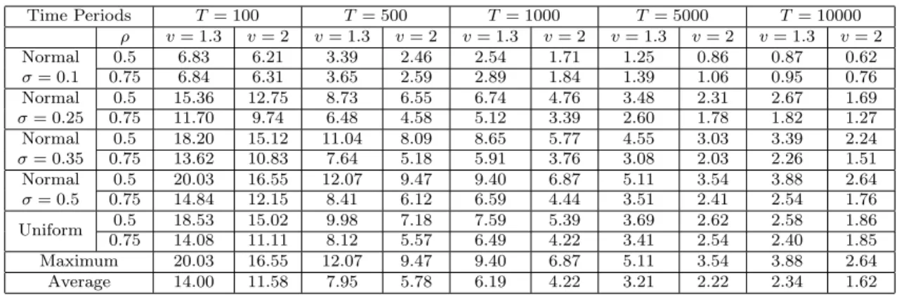
Table 2.1:Exponential Demand

Time Periods T = 100 T= 500 T = 1000 T= 5000 T = 10000 ρ v= 1.3 v= 2 v= 1.3 v= 2 v= 1.3 v= 2 v= 1.3 v= 2 v= 1.3 v= 2 Normal σ= 0.1 0.5 6.83 6.21 3.39 2.46 2.54 1.71 1.25 0.86 0.87 0.62 0.75 6.84 6.31 3.65 2.59 2.89 1.84 1.39 1.06 0.95 0.76 Normal σ= 0.25 0.5 15.36 12.75 8.73 6.55 6.74 4.76 3.48 2.31 2.67 1.69 0.75 11.70 9.74 6.48 4.58 5.12 3.39 2.60 1.78 1.82 1.27 Normal σ= 0.35 0.5 18.20 15.12 11.04 8.09 8.65 5.77 4.55 3.03 3.39 2.24 0.75 13.62 10.83 7.64 5.18 5.91 3.76 3.08 2.03 2.26 1.51 Normal σ= 0.5 0.5 20.03 16.55 12.07 9.47 9.40 6.87 5.11 3.54 3.88 2.64 0.75 14.84 12.15 8.41 6.12 6.59 4.44 3.51 2.41 2.54 1.76 Uniform 0.5 18.53 15.02 9.98 7.18 7.59 5.39 3.69 2.62 2.58 1.86 0.75 14.08 11.11 8.12 5.57 6.49 4.22 3.41 2.54 2.40 1.85 Maximum 20.03 16.55 12.07 9.47 9.40 6.87 5.11 3.54 3.88 2.64 Average 14.00 11.58 7.95 5.78 6.19 4.22 3.21 2.22 2.34 1.62

Table 2.2: Logit Demand

Time Periods T = 100 T= 500 T = 1000 T= 5000 T = 10000 ρ v= 1.3 v= 2 v= 1.3 v= 2 v= 1.3 v= 2 v= 1.3 v= 2 v= 1.3 v= 2 Normal σ= 0.1 0.5 6.80 5.62 4.35 2.30 2.63 1.63 1.26 0.89 0.85 0.63 0.75 10.09 8.34 3.42 3.67 4.42 2.67 2.15 1.60 1.45 1.15 Normal σ= 0.25 0.5 13.72 9.57 6.83 4.44 4.98 3.17 2.34 1.56 1.66 1.10 0.75 12.58 9.86 6.89 4.51 5.42 3.30 2.67 1.87 1.81 1.35 Normal σ= 0.35 0.5 17.13 12.52 8.65 6.01 6.52 4.10 3.04 1.98 2.12 1.41 0.75 13.84 10.49 7.49 4.85 5.82 3.55 2.85 2.00 1.96 1.43 Normal σ= 0.5 0.5 19.38 13.75 9.99 6.52 7.31 4.57 3.35 2.18 2.34 1.57 0.75 14.49 11.30 7.84 5.24 6.07 3.79 3.00 2.11 2.05 1.51 Uniform 0.5 21.20 15.29 9.51 6.20 7.16 4.46 3.36 2.39 2.29 1.72 0.75 17.46 14.63 10.44 6.97 8.74 5.35 4.81 3.63 3.38 2.73 Maximum 21.20 15.29 10.44 6.97 8.74 5.35 4.81 3.63 3.38 2.73 Average 14.67 11.14 7.54 5.07 5.91 3.66 2.88 2.02 1.99 1.46

Table 2.1 summarizes the results when the underlying demand curve is exponen-tial, and Table 2.2 displays the results when the underlying demand curve is logit. Combining both tables, one sees that whenT = 100 periods, on average the profit loss from the DDA algorithm falls between 11% and 14% compared to the optimal profit under complete information, in which DDA starts with no prior knowledge about the underlying demand. When T = 500, the profit loss is further reduced to between 5% and 8%. The performance gets better and better when T becomes larger. Also, it

(34)

is seen from the table that the overall performance of algorithm is better when the variance of the demand is smaller, which is intuitive.

As mentioned earlier, Theorems II.1 and II.2 continue to hold for the additive demand model ˜Dt(pt) = ˜λ(pt) + ˜t with minor modifications. Specifically, we need to modify Assumption 1 to Assumption 1A below.

Assumption 1A. The demand-price function ˜λ(p) satisfy the following conditions: (i0) pλ(p) is unimodal in˜ pon p∈ P.

(ii0) −1< ˜λ00(p)˜λ(p)

2(˜λ0₍_p₎₎2 <1, for all p∈ P.

Note that these are exactly the same assumptions made inBesbes and Zeevi (2015) for the revenue management problem, and examples that satisfy Assumption 1A include (a) linear withλ(p) = k−mp,m >0, (b) exponential withλ(p) = ek−mp_{, m >} 0, and (c) logit with λ(p) = ₁₊ek_e−k−mpmp, m >0, e

k−mp_<_{3 for all} _p_{∈ P}_.

The learning algorithm for the additive demand model is similar to that of the multiplicative demand case, except that there is no need to transform it using the logarithm of the deterministic portion of demand and the logarithm of random de-mand error. Instead, the algorithm directly estimates ˜λ(p) using affine function and computes the biased samples of the random demand error in each iteration.

2.4 Sketches of the Proof

In this section, we present the main ideas and steps in proving the main results of this chapter. In the first subsection, we elaborate on the technical issues encountered in the proofs. The key ideas of the proofs are discussed in Subsection 4.2, and the major steps for the proofs of Theorems 1 and 2 are given in Subsections 4.3 and 4.4, respectively.

(35)

2.4.1 Technical Issues Encountered

To prove Theorem 1, we will need to show

E(ˆpi+1−p∗)2 →0, _E (ˆpi+1+δi+1−p∗)2 →0, asi→ ∞; (2.11) E[(y∗−yˆi+1,1)2]→0, E[(y∗−yˆi+1,2)2]→0, as i→ ∞, (2.12)

where p∗ is the optimal solution of

max p∈P Q(p, λ(p)) = maxp∈P n peλ(p)_Ee−J(λ(p))o, where J(λ(p)) is defined as J(λ(p)) = min y∈Y n h_Ey−eλ(p)e++b_Eeλ(p)e−y+o.

However, both Q(·,·) and J(·) are unknown to the firm because all the expectations cannot be computed. To estimate J(·), in (2.8) of the learning algorithm we use the data-driven biased estimation of

J_iDD₊₁( ˆαi+1−βî+1p) = min y∈Y 1 2Ii ti+2Ii X t=ti+1 hy−eαî+1−βî+1p_eηt + +beαî+1−βî+1p_eηt₋_y + ,

and ˆpi+1 is the optimal solution of

max p∈P Q DD i+1(p,αî+1−βî+1p) = max p∈P peαî+1−βî+1p 1 2Ii ti+2Ii X t=ti+1 eηt ₋_JDD i+1( ˆαi+1−βî+1p) , in which QDD

i+1(·,·) is random and is constructed based on biased random samples ηt. To prove the convergence of the data-driven solutions to the true optimal solution, we face two major challenges. The first one is the comparison between JDD

i+1( ˆαi+1−

ˆ

(36)

replaced by a linear estimation and, due to lack of knowledge about distribution of random error, the expectation is replaced by an arithmetic average from biased samples ηt not true samples of random error t. To put it differently, the objective function forJDD

i+1 is not a sample average approximation, but a biased-sample average

approximation. The second challenge lies in the comparison of QDD

i+1(p,αˆi+1−βˆi+1p)

and Q(p, λ(p)). Since QDD_i₊₁ is a function of J_iDD₊₁ that is minimum of a biased-sample average approximation, the errors in replacing t byηt carry over toQDD_i₊₁, making it difficult to compare (ˆpi+1,yiˆ+1,1) and (ˆpi+1+δi+1,yiˆ+1,2) with (p∗, y∗). To overcome the

first difficulty, we establish several important properties of the newsvendor problem and bound the errors of biased samples (Lemmas A2, A3, A4, A8 in the Appendix). For the second, we identify high probability events in which uniform convergence of the data-driven objective functions can be obtained (Lemmas A1, A5, A6, and A7 in the Appendix).

We note that in the revenue management problem setting,Besbes and Zeevi(2015) also prove the convergence result (2.11). InBesbes and Zeevi (2015),p∗ is the optimal solution of maxp∈PQ(p, λ(p)), and ˆpi+1 is the optimal solution of maxp∈PQ(p,αˆi+1−

ˆ

βi+1p), where Q(·,·) is a known and deterministic function Q(p, λ(p)) = pλ(p). As

Besbes and Zeevi (2015) point out, their analysis extends to more general function Q(p, λ(p)) in which Q(·,·) is a known deterministic function. This, however, is not true in our setting asQ(·,·) is not known, and as a matter of fact, one cannot even find an unbiased sample average to estimate Q(·,·). Therefore, the challenges discussed above were not present in Besbes and Zeevi (2015).

2.4.2 Main Ideas of the Proof

To compare the policy and the resultant profit of DDA algorithm with that of the optimal solution, we first note that these two problems differ along several dimensions. For example, in DDA we approximate λ(p) by an affine function and estimate the

(37)

parameters of the affine function in each iteration, and we approximate the expected revenue and the expected holding and shortage costs using biased sample averages. These differences make the direct comparison of the two problems difficult. Therefore, we introduce several “intermediate” bridging problems, and in each step we compare two “adjacent” problems that differ just in one dimension.

For convenience, we follow Besbes and Zeevi (2015) to introduce notation

˘

α(z) = λ(z)−λ0(z)z, β(z) =˘ −λ0(z), z ∈ P. (2.13)

We proceed to prove (2.11) as follows:

E(p∗−pˆi+1)2 ≤ _E p ∗₋ p α(ˆ˘ pi),β(ˆ˘ pi) | {z }

Comparison of problems CI and B1 Lemma A1 (2.14) + p α(ˆ˘ pi), ˘ β(ˆpi) −p˜i+1 ˘ α(ˆpi),β(ˆ˘ pi) | {z }

Comparison of problems B1 and B2 Lemma A5 + + p˜i+1 ˘ α(ˆpi),β(ˆ˘ pi) −pˆi+1 | {z }

Comparison of problems B2 and DD Lemma A6 and Lemma A7

2

,

where the two new pricesp ·,·) and ˜pi+1(·,·) are the optimal solutions of two bridging

problems. Specifically, we letp α, β

denote the optimal solution for the first bridging problem B1 defined by Bridging Problem B1: max p∈P ( peα−βp_Ee−min y∈Y h_Ehy−eα−βpei + +b_Eheα−βpe−yi +) , (2.15)

(38)

defined by Bridging Problem B2: max p∈P ( peα−βp 1 2Ii ti+2Ii X t=ti+1 et ! (2.16) −min y∈Y 1 2Ii ti+2Ii X t=ti+1 h y−eα−βpet+₊_{b e}α−βp_et ₋_y+ ) .

Moreover, for given p ∈ P, we let y(eα−βp_{) denote the optimal order-up-to level for} problem B1, and ˜yi+1(eα−βp) denote the optimal order-up-to level for problem B2.

By Lemma A2 in the Appendix, the objective functions for problems B1 and B2 are unimodal in p after minimizing overy ∈ Y when β >0.

Comparing (2.15) with (2.4), it is seen that problem B1 simplifies problem CI by replacing the demand-price functionλ(p) by a linear functionα−βp, while problem B2 is obtained from problem B1 after replacing the mathematical expectations in problem B1 by their sample averages, i.e., problem B2 is the SAA of problem B1. Comparing (2.16) with (2.8), it is noted that problems B2 and DD differ in the coefficients of the linear function as well as the arithmetic averages. More specifically, in B2 the real random error samplest,t=ti+ 1, . . . , ti+ 2Ii, are used, while in problem DD, biased error samplesηtare used in place oft, t=ti+ 1, . . . , ti+ 2Ii. Furthermore, note that the optimal prices for problems CI and B1, p∗ and p α(ˆ˘ pi),β(ˆ˘ pi)

, are deterministic, but the optimal solutions of problems B2 and DD, ˜pi+1 α(ˆ˘ pi),β(ˆ˘ pi)

and ˆpi+1, are

random. Specifically, ˜pi+1 α(ˆ˘ pi),β(ˆ˘ pi)

is random because t is random, while ˆpi+1

is random due to demand uncertainty from periods 1 to ti+1. Hence, to show the

right hand side of (2.14) converges to 0, we will first develop an upper bound for

p∗−p α(ˆ˘ p_i),β(ˆ˘ p_i)

by comparing problems CI and B1, and the result is presented

in Lemma A1. Since ˜pi+1( ˘α(ˆpi),β(ˆ˘ pi) is random, we compare the two problems B1 and

B2 and show the probability that p α(ˆ˘ pi),β(ˆ˘ pi)

−pi˜+1 α(ˆ˘ pi),β(ˆ˘ pi)

(39)

small number diminishes to 0 in Lemma A5. Similarly, in Lemma A6 and Lemma A7 we compare problems B2 and DD and show the probability thatp˜i+1 α(ˆ˘ pi),β(ˆ˘ pi)

− ˆ

pi+1

exceeds some small number also diminishes to 0. Finally, we combine these

several results to complete the proof of (2.11). The idea for proving (2.12) is similar, and that also relies heavily on the two bridging problems (Lemmas A6, A7, and A8). The detailed proofs for Theorem 1 and Theorem 2 are given in Subsections 4.3 and 4.4.

In the subsequent analysis, we assume that the space for feasible price, P, and the space for order-up-to level, Y, are large enough so that the optimal solutions p∗ and optimaly(eλ(p)_{) over}

R+for givenp∈ P for problem CI fall intoP andY, respectively;

and for given q ∈ P, the optimal solutions p α(q),˘ β(q)˘ and y eα˘(q)−_β˘₍_q₎_p

for given p ∈ P over _R+ for problem B1 fall into P and Y, respectively. Note that both

problem CI and problem B1 depend only on primitive data and do not depend on random samples, hence these are mild assumptions. We remark that our results and analyses continue to hold even if these assumptions are not satisfied as long as we modify Assumption 1(ii) to ∂p α(z),˘ β(z)˘

/∂z < 1 for z ∈ P. This condition

reduces to Assumption 1(ii) if the optimal solutions for problem CI and problem B1 satisfy the feasibility conditions described above.

We end this subsection by listing some regularity conditions needed to prove the main theoretical results.

Regularity Conditions:

(i) y(eλ(q)) and y eα˘(q)−β˘(q)p are Lipschitz continuous on q for given p ∈ P, i.e., there exists some constant K1 >0 such that for any q1, q2 ∈ P,

y(eλ(q1))−y(eλ(q2)) ≤K₁|q₁−q₂|, (2.17) y e ˘ α(q1)−β˘(q1)p₋_{y e}α˘(q2)−β˘(q2)p ≤K1|q1−q2|. (2.18)

(40)

(ii) G(p,y(e¯ λ(p)_{)) has bounded second order derivative with respect to} _p_{∈ P}_.

(iii) _E[Dt(p)]>0 for any price p∈ P.

(iv) λ(p) is twice differentiable with bounded first and second order derivatives on p∈ P.

(v) The probability density function f(·) of ˜t satisfies min{f(x), x∈[l, u]}>0. It can be seen that all the functions in Example 1 satisfy the regularity conditions above with appropriate choices ofpl _and _ph_.

2.4.3 Proof of Theorem 1

The proofs for the convergence results are technical and rely on several lemmas that are provided in the Appendix. In this subsection, we outline the main steps in establishing the first main result, Theorem 1.

Convergence of pricing decisions. To prove the convergence of pricing

deci-sions, we continue the development in (2.14) as follows:

E(p∗−pî+1)2 ≤ _Eh p ∗₋ p α(ˆ˘ pi),β(ˆ˘ pi) + p α(ˆ˘ pi), ˘ β(ˆpi) −p˜i+1 α(ˆ˘ pi),β(ˆ˘ pi) + p˜i+1 α(ˆ˘ pi), ˘ β(ˆpi) −pî+1 2i ≤ _Ehγ|p∗−pî|+ p α(ˆ˘ pi), ˘ β(ˆpi) −p˜i+1 α(ˆ˘ pi),β(ˆ˘ pi) + p˜i+1 α(ˆ˘ pi), ˘ β(ˆpi) −pî+1 2i ≤ 1 +γ2 2 E(p∗ −pî)2 +K2E p α(ˆ˘ pi), ˘ β(ˆpi) −p˜i+1 α(ˆ˘ pi),β(ˆ˘ pi) + p˜i+1 α(ˆ˘ pi), ˘ β(ˆpi) −pî+1 2 ≤ 1 +γ2 2 E(p∗ −pî)2 +K3E p α(ˆ˘ pi), ˘ β(ˆpi) −p˜i+1 α(ˆ˘ pi),β(ˆ˘ pi) 2 ˘ 2

(41)

where the first inequality follows from the expansion in (2.14), the second inequality follows from Lemma A1, and the third inequality is justified by γ <1 in Lemma A1 and some constant K2, and the last inequality holds for some appropriately chosen

K3 because of the inequality (a+b)2 ≤2(a2+b2) for any real numbersa and b.

To bound _Ep α(ˆ˘ p_i),β(ˆ˘ p_i) −p˜i+1 α(ˆ˘ pi),β(ˆ˘ pi) 2 in (2.19), by Lemma A5 one has, for some constant K4,

E p α(ˆ˘ pi), ˘ β(ˆpi) −p˜i+1 α(ˆ˘ pi),β(ˆ˘ pi) 2 ≤K₄2 +∞ Z 0 5e−4Iiξ2_dξ ₌ 5π 1 2K2 4 4I 1 2 i . (2.20) And to bound _E pi˜+1 α(ˆ˘ pi), ˘ β(ˆpi)−piˆ+1 2

in (2.19), by Lemma A6 and Lemma A7, wheniis large enough (greater than or equal to i∗ defined in the proof of Lemma A7), for some positive constants K5, K6, and K7 one has

Substituting (2.20) and (2.21) into (2.19), one has

E(p∗−pˆi+1)2 ≤ 1 +γ2 2 E(p∗−pˆi)2 +K8I −1 2 i .

(42)

Letting 1+₂γ2 =θ, we further obtain E(ˆpi+1−p∗)2 ≤ θi(ˆp1−p∗)2+K8 i−1 X j=0 θjI− 1 2 i−j ≤K9(v− 1 2)i i−1 X j=0 θj(v12)j.(2.22)

We choosev >1 that satisfiesθv12 <1, then there exists a positive constantK₁₀such

that Pi−1

j=0θ

j_(v1₂₎j _≤_K

10, therefore, for some constants K11 and K12,

E(ˆpi+1−p∗)2 ≤K11(v− 1 2)i ≤K 12I −1 2 i . (2.23)

Moreover, we have, for some positive constant K13,

E(ˆpi+1+δi+1−p∗)2 ≤2_E(ˆpi+1−p∗)2 + 2δ2_i₊₁ ≤K13I −1 2 i →0, as i→ ∞. (2.24) This completes the proof of (2.11). Because mean-square convergence implies convergence in probability, this shows that the pricing decisions from DDA converge top∗ in probability.

Convergence of inventory decisions. To prove yt converges to y∗ in

(43)

K14, we have E h y∗ −yˆ_i₊₁_,₁ 2i ≤ _Eh y e λ(p∗) −y(eλ( ˆpi+1)₎ + y e λ( ˆpi+1)₋_{y e}α˘( ˆpi+1)−β˘( ˆpi+1) ˆpi+1₎ + y e ˘ α( ˆpi+1 −_β˘_{( ˆ}_p_i₊₁_{) ˆ}_p_i₊₁ )−y eα˘( ˆpi)−β˘( ˆpi) ˆpi+1 + y e ˘ α( ˆpi)−β˘( ˆpi) ˆpi+1₋_y_˜ i+1 eα˘( ˆpi)− ˘ β( ˆpi) ˆpi+1 + y˜i+1 e ˘ α( ˆpi)−β˘( ˆpi) ˆpi+1₋_y_ˆ i+1,1 2i ≤ K14E h y e λ(p∗₎ −y(eλ( ˆpi+1)₎ 2 | {z }

Difference betweenp∗and ˆpi+1

+ y e λ( ˆpi+1)₋_{y e}α˘( ˆpi+1)−β˘( ˆpi+1) ˆpi+1₎ 2 | {z } Zero (2.25) + y e ˘ α( ˆpi+1)−β˘( ˆpi+1) ˆpi+1₋_{y e}α˘( ˆpi)−β˘( ˆpi) ˆpi+1 2 | {z }

Difference between ˆpi+1and ˆpi

+ y e ˘ α( ˆpi)−β˘( ˆpi) ˆpi+1₋_y_˜ i+1 eα˘( ˆpi)− ˘ β( ˆpi) ˆpi+1 2 | {z }

Comparison of problems B1 and B2 Lemma A8 + y˜i+1 e ˘ α( ˆpi)−β˘( ˆpi) ˆpi+1₋_y_ˆ i+1,1 2 | {z }

Comparison of problems B2 and DD Lemma A6 and Lemma A7

i

.

We want to upper bound each term on the right hand side of (2.25). First, it follows from (2.17) that, for some constantK15 it holds

E y e λ(p∗₎ −y eλ( ˆpi+1) 2 ≤K15E|p∗−piˆ+1 |2 .

By definition of ˘α(p) and ˘β(p) in (2.13) one has ˘α(ˆpi+1)−β(ˆ˘ pi+1)ˆpi+1 =λ(ˆpi+1), thus

the second term on the right hand side of (2.25) vanishes. For the third term, we apply the Lipschitz condition ony eα˘(q)−β˘(q)p

in (2.18) to obtain, for some constants K16 and K17, E y e ˘ α( ˆpi+1)−β˘( ˆpi+1) ˆpi+1₋_{y e}α˘( ˆpi)−β˘( ˆpi) ˆpi+1 2 ≤ K16E |pˆi+1−pˆi |2 ≤ K17E |p∗−piˆ |2 +|p∗−piˆ+1 |2 .

(44)

By Lemma A8, we have, for some constants K18 and K19, E y e ˘ α( ˆpi)−β˘( ˆpi) ˆpi+1₎₋_y_˜ i+1 eα˘( ˆpi)− ˘ β( ˆpi) ˆpi+1 2 ≤ K₁₈2 +∞ Z 0 2e−4Iiξ_dξ_≤ K19 Ii , (2.26)

and by Lemma A6 and Lemma A7 one has, for some constant K20,

Summarizing the analyses above we obtain, for some constants K21 and K22,

E h y∗−yî+1,1 2i ≤ K21E |p∗−pî+1 |2 +|p∗−pî |2 +K21I −1 2 i ≤ K22I −1 2 i (2.27) → 0 as i→ ∞,

where the second inequality follows from the convergence rate of the pricing decisions. Similarly, we obtain E h y∗−yˆi+1,2 2i ≤K22I −1 2 i →0, as i→ ∞.

We next show that _E[(y∗−yt)2]→0 ast→ ∞. It suffices to prove this for (a)t∈ {ti+1+ 1, . . . , ti+1+Ii+1},i= 1,2, . . ., and for (b)t∈ {ti+1+Ii+1+ 1, . . . , ti+1+ 2Ii+1},

i= 1,2, . . .. We will only provide the proof for (a).

The inventory order up-to level prescribed from DDA for periods t ∈ {ti+1 +

(45)

t. Consider the event that the second order up-to level of learning stage i, ˆyi,2, is

achieved during periods {ti +Ii + 1, . . . , ti + 2Ii}. Since ˜λ(ph)l ≤ Dt ≤ λ(p˜ l)u, it follows from Hoeffding inequality1 _{that for any} _{ζ >}_0,

P ( _t_i₊₂_I_i X t=ti+Ii+1 Dt≥E " _t_i₊₂_I_i X t=ti+Ii+1 Dt # −ζ ) ≥1−exp − 2ζ 2 Ii(˜λ(pl)u−λ(p˜ h)l)2 .(2.28) Letζ = ˜λ(pl)u−˜λ(ph)l(Ii) 1 2 _(log_I i) 1

2 _{in (2.28), then one has}

P ( _t_i₊₂_I_i X t=ti+Ii+1 Dt ≥IiE[Dti+Ii+1]− λ(p˜ l )u−˜λ(ph)l(Ii) 1 2 _(log_I i) 1 2 ) ≥1− 1 I2 i . (2.29)

By regularity condition (iii), _E[Dti+Ii+1]>0, thus when iis large enough, we will

have 1 2IiE[Dti+Ii+1]≥ ˜λ(p l_)u₋_λ(p_˜ h_)l (Ii) 1 2 (logI i) 1 2 .

Hence it follows from (2.29) that, wheni is large enough, we will have

P ( _t i+2Ii X t=ti+Ii+1 Dt≥ 1 2IiE[Dti+Ii+1] ) ≥1− 1 I2 i . (2.30) Define event A1 = ( ω : ti+2Ii X t=ti+Ii+1 Dt≥ 1 2IiE[Dti+Ii+1] ) ,

then (2.30) can be rewritten as

P(A1)≥1−

1 I2

i .

1_{If the random demand is not bounded, then the same result is obtained under the condition}