A Survey on Different Machine Learning Techniques for Air Quality Forecasting for Urban Air Pollution

A Survey on Different Machine Learning

Techniques for Air Quality Forecasting for Urban

Air Pollution

Sayali Nemade1, Chandrashekhar Mankar2 2

Assist. Prof., 1Department of CSE, SSGMCE, Shegaon, SGBAU University, Amravati, Maharashtra, India

Abstract: The delinquent of air pollution has become a staid concern in developed as well as developing republics. Distressing human’s respiratory and cardiovascular system, air pollution is the origin for increased impermanence and increased risk for diseases for the inhabitants.Particulate matter (PM 2.5) needs more responsiveness. When its level is in elevation in the air, it causes solemn issues on people’s health. Hence, we need to control it by uncompromisingly keeping a trail of its levels in air.

With cumulative air pollution, we need to implement proficient air quality monitoring models which collect evidence about the deliberation of air pollutants and provide assessment of air pollution in apiece expanse. Hence, evaluating air quality and its

prediction is an imperative research capacity. This paper is basically a little contribution towards this challenge. We compare

four unpretentious machine learning algorithms, linear regression, naïve bayes, support vector machine and random forest. Enactment of these algorithms can undeniably be helpful to predict air pollutants levels ahead of time.

Keywords: Air Quality, Machine Learning, Linear Regression, Naïve Bayes, Support Vector machine, Random Forest.

I. INTRODUCTION

Air is the integral fragment for the way of life and endurance of the entire life on this planet. The whole shebang including animals, plants and humans need air for their subsistence. Thus, all living organisms need virtuous quality of air which is deprived of damaging experiences to carry on their life. It is found that the elder people and fledgling children are affected by air effluence in inordinate amounts. Foremost outdoor air pollutants in conurbations take account of ozone (O3), particle matter (PM), sulphur dioxide (SO2), carbon monoxide (CO), nitrogen oxides (NOx), volatile organic compounds (VOCs), pesticides, and metals, among others [1,2]. Air pollutants cause pro tem effects such as eye, snozzle, and oesophagus irritation, nuisances, hypersensitive reactions, and upper respirational toxicities. Abiding health effects caused by air pollution include lung malignancy, brain mutilation, liver impairment, kidney destruction, heart ailment, and breathing sickness. It also complements to the diminution of the ozone stratum, which protects the Globe from sun's UV flickers. Increased impermanence and indisposition rates have been found in connotation with augmented air pollutants (such as O3, PM and SO2) concentrations [2–4]. Bestowing to the testimony from the American Lung Association [5], a 10 parts per billion (ppb) increase in the O3 mingling ratio might cause over 3700 premature bereavements per annum in the United States (U.S.). Chicago, as intended for many other megacities in U.S., has thrashed with air pollution as an upshot of industrialization and urbanization. Although Ozone forerunners (such as VOCs, NOx, and CO) emanations have ominously decreased ever since the late 1970s, O3 levels in Chicago have not been in acquiescence with standards customary by the Environmental Protection Agency (EPA) to care for community health [5]. Particulate matter can be either imitation or sincerely befalling. Some specimens include dirt, cinders and sea-spray. Particulate matter is emanated during the incineration of fuels, such as for power generation, inland heating and in means of transportation engines. Particulate matter fluctuates in magnitude (i.e. the diameter or thickness of the particle). PM2.5 refers to the bulk per cubic meter of air of constituent part with a size (span) by and

large less than 2.5 micrometers (μm) [6]. PM2.5 which is readily known as suspended fine particulate matter (2.5 micrometers is

one 400th of a millimeter). Particle proportions is perilous in seminal the particle deposition whereabouts in the human respiratory system [6]. PM2.5, stating to particles with a diameter less than or equal to 2.5 µm, has been an amassed concern, as these particles can be deposited into the lung gas-exchange region, the alveoli [7]. Hence, air pollution is one of the most important and serious disquiet for us in our day. So directing on this dispute, in the former decades, many researchers have spent lots of time on revising

and developing different models and methods in air quality exploration and evaluation. Evaluation of air quality has been

shepherded usingunadventurous approaches in all these eons.

Machine Learning is the prevalent upswing now. Machine learning is an important turf where system which apparatuses artificial

machine learning to predict air quality index, was this knack of acclimatizing of machine learning (ML) algorithms. Machine learning approaches have been rising in excess of 60 years and have accomplished remarkable success in multiplicity of areas

[8-13].In this paper four machine learning techniques are paralleled. It is sustained by recent literature review and study on the existing

publicationswhich focused on air quality evaluation and prediction via these approaches. The foremost focus is to provide a an inclusive picture of the cosmic research work and useful criticism on thecurrent up-to-the-minute on pertinent big data approaches andmachine learning techniques for air quality evaluation andextrapolation.

II. AIR QUALITY EVALUATION A. Sorts of Air Pollutants

Appraising air quality is an important way to monitor and control air contamination. The peculiarity of air quality affect its appropriateness for a certain employment. An explicit clutch of air contaminants, called criteria air pollutants, are conjoint all the way through the United States. These pollutants can root health issues, can harm the environs and can cause health deterioration. Majorly heart-rending contaminants are [14]:-

1) Carbon monoxide: Carbon monoxide is a color-depriving and smell-depriving gas. It builds up in air when fuels containing

carbon are parched in depressed oxygen conditions. Carbon monoxide syndicates with other pollutants in the air to form treacherously detrimental ground-level ozone. It does not have any good impression on atmosphere at a widespread level. Gulp of air of carbon monoxide at high concentrations can be terminal because it thwarts the conveyance of oxygen in the blood all over the body.

2) Sulphur dioxide: It is imperceptible and has a nauseating, sharp aroma. It is twisted mostly by burning of fossil fuels

particularly from power stations, converting wood mush to paper, manufacturing of sulphuric acid, incineration of refused products and casting. Sulphur dioxide when huffed exasperates the nose, gullet, and air lane to cause coughing, wheeziness, quickness of breath, or a snug feeling in the chest. The effects of sulphur dioxide are felt very hastily and most people would feel the foulest threatening signs in 10 or 15 minutes subsequently inhaling it. Those most at risk of emergent problems if they are bare to sulphur dioxide are people with asthma or analogous conditions.

3) Nitrogen Dioxide: Its manifestation in air can be prime to the realization and amendment of other air pollutants, such as ozone

and particulate matter, and acid deluge. Readings on human populations indicate that long-term exposure to NO2 levels possibly will drop lung function and increase the risk of respirational indications such as acute bronchitis and cough and imperturbability, particularly in progenies and also affect transience. Folks with asthma and children in broad-spectrum, are painstaking to be further predisposed to NO2 exposure.

4) Particulate matter (PM): It is a concoction of compacted constituent part and liquefied condensations found in the air. Some

particles, such as dust, dirt, soot, or smoke, are large enough to be discernible by way of the bare eye. Others are so trifling that they can only be spotted using a compound microscope.

a) PM 10: inhalable particles, with diameters that are by and large 10 micrometres and less significant.

b) PM 2.5: fine inhalable specks, with diameters that are in the main 2.5 micrometres and less important. Particulate matter contains so minuscule solid or liquid droplets that are so trivial that they can be gulped and cause serious wellbeing problems. Particles less than 10 micrometres in diameter cause the biggest problems because they can get to the bottom of your lungs, and some can even get into your blood vessels.

B. Air Quality Criterions

EPA curriculums are basically bring about by OAQPS to mend air quality in capacities where the in progress eminence is not

obnoxious and to prevent depreciation in areas where the air is at liberty of impureness. Intended for this very reason OAQPS

established the National Ambient Air Quality Standard (NAAQS) for each of the criteria of air noxious waste. There are basically

two natures of standards - primary and secondary.

1) Primary Standards: They protect in contradiction of detrimental health paraphernalia;

2) Secondary Standards: They protect in contradiction of impairment to farm yields and plant life and destruction to edifices. Paraphernalia of different pollutants are altered so the NAAQS standards are also different for different pollutants. Some pollutants

have standards for both long-standing and stop gap effects. As different pollutants have different effects, the NAAQS [15] standards

According to the researchers E. Kalapanidas and N. Avouris [16], illustration of air pollution singularities till now has been predominantly based on dispersal models that deliver juxtaposition of the physicochemical manners counted in. As the convolution of these models have augmented since the preceding ages, use of these techniques in the edging of real-time atmospheric pollution specialist care seems to be not apposite in terms of performance, input statistics requirements and conformism with the time constrictions of the problem. In its place, human connoisseurs’ knowledge has been basically smeared in Air Quality Operational Centres for the real-time decrees required, while mathematical models have been used customarily for off-line trainings of the trepidations involved. As per them, air pollution portent have been measured by using physical veracity as the start theme. Kalapanidas et al. [16] expounded effects on air pollution solitarily from meteorological topographies such as temperature, wind, precipitation, solar radiation, and humidity and classified air pollution into different levels (low, med, high, and alarming) by means

of an easy learning methodology, the case-based reasoning (CBR) system. Athanasiadis et al. [17] has given the α-fuzzy lattice

classifier to foretell and catalog Ozone deliberations into three echelons (low, mid, and high) on the foundation of meteorological features and other pollutants such as SO2, NO, NO2, and so on.

Table I: NAAQS Table Grades ALL Criteria Contaminants and Standards [15]

Pollutant Primary/

Secondary

Averaging Time Level Form

Carbon

Monoxide (CO)

Primary Standard 8 Hrs 9 parts per

million

Should not be exceeded more than once per year

1 Hr 35 parts per

million

Lead (Pb) Both Primary and

Secondary

Undulating 3 month mediocre

0.15 µg/m3 Should not be exceeded

Nitrogen Dioxide (NO2)

Primary Standard 1 Hr 100 parts per

billion

98th percentile of 1-hr day-to-day Concentrated concentrations, be more or less over 3 years

1 Yr 53 parts per

billion

Yearly Mean

Ozone (O3) Both Primary and

Secondary Standard

8 Hrs 0.07 parts per

million

Twelve-monthly fourth-highest daily maximum 8 hrs

concentration, be in the region of over 3 years

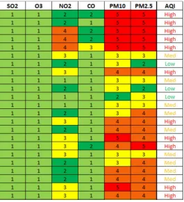
Kurt and Oktay [18] modelled topographical acquaintances into a neural linkage model and predicted per diem concentration levels of SO2, CO, and PM10 3 days in advance. Other researchers have toiled on prophesying concentrations of contaminants. Corani [19] drove on training neural network models to envisage hourly O3 and PM10 concentrations on the foundation of facts from the aforementioned day. We have one central factor called air quality index (AQI) which measures air quality in a constituency as revealed in Table II. It is ultimately a numeral used by government bureaus to let know the public on how adulterated the air is currently or how polluted it will be in nigh future. As the AQI increases, an expectedly hefty percentage of the human population is in the offing to be exposed, and people may experience progressively more severe health issues. Different republics have their vastly regarded air quality indices, corresponding to different national air quality criterions.

TABLE II: AQI TAXONOMY [15]

AQI Air Pollution Level

0-50 Excellent

51-100 Good

101-150 Lightly Polluted

151-200 Moderately Polluted

201-300 Heavily Polluted

Figure 1 AQI according to attribute values

III.LINEAR REGRESSION

Beforehand we get familiar with what in point of fact linear regression is, we need get ourselves at ease with regression. Regression is a method of signifying a target value grounded on sovereign clairvoyants. This method is habitually used for foretelling and finding out cause-and-effect liaison flanked by variables. Regression modus operandi for all intents and purposes show a discrepancy in the face of the variety of relationship we fixed up between dependent and independent variables and the number of independent variables jumble-saled.

Figure 2. Linear Regression

A. Cost Function

The cost function arrange for great backing to pattern out the unsurpassed in the cards values for a_0 and a_1 which would fortify to the optimum fit line for the data points. Since we dearth the best values for a_0 and a_1, we need to transfigure this search problem into a minimization delinquent where we would single-mindedly focus on minimizing the blunder between the predicted value and the tangible value.

We choose the above function to curtail. The variance between the predicted values and the pulverized values measures the error difference. We take the square of the error difference and then we take entirety of the inclusive data points and then distribute that value by the over-all number of data points. This will contribute the average squared error over all the data points. Therefore, this cost function can also be devised as the Mean Squared Error (MSE) function. Now, we will make consumption of this MSE function for the amendment of the values of a_0 and a_1 such that the MSE value amalgamates at the modicums. Now and again the cost function can be a non-convex function someplace you could culminate at a local minima but for linear regression, it at all times has to be a convex function.

Figure 3 Convex (left) and Non-Convex (right) Function

B. Gradient Descent

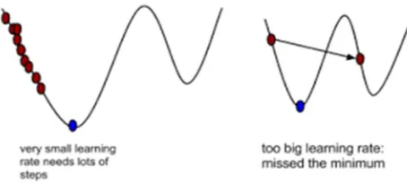
The second crucial conception needed to plumb linear regression is gradient descent. Gradient descent is a method countenancing us to bring upto date a_0 and a_1 to condense the cost function MSE. The impression is that we flinch with some values for a_0 and a_1 and then we change these values over and over again to reduce the cost. Gradient descent comforts us on by what method we can change the values.

Figure 4 Learning rates to reach the minima

C. Pros of Linear Regression

1) Linear regression is a tremendously simple method. It is quite an informal and spur-of-the-moment to use and cognize.

2) In addition, it works in maximum of the circumstances. Even when it doesn’t apt the data faithfully, we can use it to treasure

trove the nature of the rapport between the two variable.

D. Cons of Linear Regression

1) By its demarcation, linear regression only prototypes relationships between dependent and independent variables that are

undeviating. It takes into contemplation that there is a straight-line relationship between them which is indecent on occasion. Linear regression is very profound to the discrepancy in the data.

2) What if most of your data lies in the assortment 0-10. If because of any intention only one of the data item approaches out of the

range, say for example 15, this significantly have impact on the regression quantities.

3) Added shortcoming is that if the number of constraints used is less than the number of illustrations presented then the model

flinches to model the noise rather than the liaison we set up between the dependent and independent variables.

IV.NAÏVE BAYES

Naive Bayesian classifier can be thought of as an arithmetical method that can predict class membership possibilities such as the odds that a given tuple is in the right place to a particular class. Bayesian classifier is based on the Bayes proposition and it takes on that the effect of a trait value on a given class is self-regulating of the values of the further attributes. This conjecture is called class conditional independence. It can be embraced to take back to first principles the computations involved in it and in this sagacity, is called as "naive". In unpretentious rapports, a naive Bayesian classifier take responsibility that the manifestation (or absenteeism) of an exacting feature of a class is disparate to the presence (or nonappearance) of any supplementary feature. Depending on the definite nature of the probability model, naive Bayesian classifier can be tailored very efficiently in a supervised learning environment. Countless concrete solicitations gives parameter assessment for Naive Bayes models that uses the method of maximum liability; in other words, one can grind with the naive Bayes model devoid of having to work by way of Bayesian probability or using any Bayesian ways and means. Heedlessly their ingenuous design and in all probability misleading conventions, Naive Bayes classifiers often work much better in many multifaceted physical world than one might presume. Most contemporary breakdown of the Bayesian classification problem has revealed that there might be some conjectural reasons for the unmistakably irrational efficacy of naive Bayesian classifiers. One of the plus of the naive Bayesian classifier is that it entails quite a small extent of training data to estimate the considerations (means and inconsistencies of the variables) indispensable for classification. As we requisite to assume independent variables, only the variances of the variables for each class are enforced to be strongminded and not the all-inclusive covariance matrix. The Naive Bayesian classifier is reckless and amassed and can covenant with distinct and unremitting attributes and has topnotch performance in real-life glitches. Naive Bayesian classifier algorithm can be arrayed efficaciously by enabling it to disentangle classification problems while recollecting all recompenses of naive Bayesian classifier. The comparison of performance in various dominions of materials classes gives the compensations of continual learning and indorses its application to further learning algorithms. The naive Bayesian algorithm [20] is specified as follows:

Input should be a Training Data Set D with their related class tags. Output should be a Classification of Classes. Method

1) Training Set D., Initialize X with one component.

2) If P (C i /X) > P (Cj /X) for all 1 ≤ j ≤ m: j≠ i. Maximize P (Ci /X).

3) Calculate the value of P ( Ci/X) = (P (X/Ci) P(Ci))/ P (X)

4) P (X/Ci) P (Ci) needs to be maximized.

5) P (X/C) = ∑ ( ) = P(X1/Ci)× P(X2/Ci)× P(X3/Ci)×……. ×P(Xn/Ci)

Value of Attribute Ak for tuple X.

6) If ( Ak is categorical) then P (X/Ci) P(Ci)

Else P (X/Ci) = g {Xk, µCi, σCi}

7) To predict the value of class label X calculate P (X/Ci) P(Ci) such that P (X/Ci) P(Ci) must be greater than P (X/Cj) P(Cj) for all 1

≤ j ≤ m : j≠ i.

A. Pros of Naïve Bayes Classifier

1) It is to a certain extent a relaxed and fast to predict class of test data set. It also carries out well in multi class extrapolation 2) When a case of conjecture of unconventionality holds, a Naive Bayes classifier performs superior as equated to further models such as logistic regression and you need quite not as much of training data.

3) It performs well in incident of resounding input variables compared to mathematical variable(s). For a numerical variable, unvarying dissemination can be assumed (bell curvature, which affords for a strong assumption).

B. Cons of Naïve Bayes Classifier

1) Uncertainty a grading variable has a grouping (in test data set), which was not to be grasped in training data set, then model will

ascribe a 0 (zero) probability and will not be able to make a prediction. This is time and again acknowledged as “Zero Frequency”. To solve this, we can make expenditure of the levelling techniques. Unique of the simplest levelling techniques is known as Laplace estimation.

2) On the additional side Naive Bayes is also notorious as an unscrupulous estimator, so the probability harvests

from predict_proba are not to be taken too earnestly.

3) Another snag of Naive Bayes is the deductions of independent prediction dynamics. In tangible life, it is just about beyond the

restraints of prospect to obtain a set of prediction influences which are downright independent.

V. RANDOM FOREST

In random forest as projected by Breiman, a random vector θk is generated, self-governing of the preceding random vectors θ1, ... ,

θk-1 but with the corresponding distribution; and a tree is grown by making use of the training data set and θk , which in seizure

gives in a classifier h(x, θk) where x is an input vector. In indiscriminate miscellany θ consists of a number of independent random

numerals between 1 and K. The nature, superiority and altitudinal property of θ depends on its use in tree edifice. When a large

number of trees are engendered, they vouch for the most popular class. This procedure is called random forest. A random forest is

fundamentally a sort of classifier that consists of a cluster of tree-structured classifiers {h(x, θk), k=1 ...} where the {θk} are

autonomous indistinguishably distributed random vectors and each tree put forth a unit pronouncement for the most popular class at

input x. Given a group of classifiers h1 (x), h2 (x)... hk (x), and with the training customary that is pinched at random from the

distribution of the random vector Y, X, define the margin function as Mg (X, Y) = avk I (hk (X) =Y) maxjyavk I (hk (X) = j) where I

(•) is the indicator function. The margin can measure the magnitude to which the average numeral of votes at X, Y for the right class

exceeds the average amount of vote for any further class. The loftier is the margin, the more is the pledge in the classification. The

generalization error is given by PE* = PXY (mg(X, Y) < 0) where the subscripts X, Y signpost that the probability is over the X, Y

space. Traditionally in random forest, hk (X) = h(X, θk). In lieu of a large number of trees, it streams from the Strong Law of Large

Numbers and the tree structure that: As the number of trees upsurges, for almost assuredly all structures θ1 ….PE* congregates to

PXY (P θ (h(X, θ) =Y) maxj yP θ (h(X, θ)= j) < 0). The convergence of the directly above equation elucidates why random forest do

not get the superior of as additional trees are added, but then again produce an off-putting value of the generalization miscalculation. The strategy in employment to achieve these culminations is as follows:

1) To preserve individual error truncated, we prerequisite to grow trees to thorough going profundity.

2) To keep residual correlation low, randomize by the use of

a) Propagate each tree on a bootstrap tester from the training data.

b) Insist on m<< p (the numeral of covariates). By the side for each node of every single tree select m covariates and pick the best

splitting of that node proceeding these covariates.

A. Imperative Hyperparameters

The hyperparameters in random forest are either used to upsurge the prophetic supremacy of the model or to mark the model quicker. 1) Increasing the Predictive Authority: Primarily, there exists the n_estimators hyperparameter, which is just the numeral of trees

2) Increasing the Models Promptness: The n_jobs hyperparameter articulates the engine exactly how many processors it is tolerable to use. Uncertainty it has an assessment of 1, it can solitarily custom one processor. A significance of “-1” revenues that there is unquestionably not bounds. Random_state marks the model’s productivity replicable. The archetypal will always reap the equivalent results when it has a persuaded value of random_state and if it has been prearranged the alike hyperparameters and the same keeping fit statistics. To sum up, there is the oob_score (correspondingly termed oob sampling), which is a random forest fractious corroboration routine. In this specimen, about one-third of the data is not castoff to train the model and can be used to gauge its performance. These mockups are so-called the out of bag testers. It is precise parallel to the leave-one-out cross-validation method, but very nearly on no account additional computational encumbrance goes laterally with it.

B. Pros of Random Forest

1) One of the pro of random forest is that it can be used in cooperation with both regression and classification tasks and that it’s easy

to be competent to see the relative importance it contributes to the input features.

2) Random Forest is also considered as within reach and easy to use algorithm, because its default hyperparameters every so often

produce a virtuous prediction result. The number of hyperparameters is quite not that extraordinary and they are indeed straightforward to apprehend.

C. Cons of Random Forest

1) One of the immense glitches in machine learning is overfitting, but peak of the stretch this won’t take place that tranquil in the

direction of a random forest classifier. That is for the reason that if there are an ample trees in the forest, the classifier will not blatant the model.

2) The leading inadequacy of Random Forest is that a large number of trees can mark the algorithm dawdling and ineffectual for

real-time predictions. In the foremost, these algorithms are quite debauched to train, but quite leisurely to build predictions once they have been trained. A more scrupulous prediction requires more trees, which can actually result in a leisurelier model. In most hands-on applications the random forest algorithm is profligate enough, but there will undoubtedly be status quo where run-time enactment is of more prominence and other approaches would be certain.

3) Random Forest is a predictive demonstrating gizmo and not an eloquent tool. In short this revenues, if you are looking for a

narrative of the affiliations in your data, other approaches would be elite.

VI.SUPPORT VECTOR MACHINES

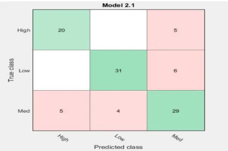
Figure 5 Confusion matrix of topmost certainty of SVM

A. Pros of SVM

1) SVMs are very virtuous when we have no inkling about the data.

2) It works in good health with even amorphous and semi well-thought-out data resembling text, Images and trees.

3) It weighbridges reasonably well towards high dimensional statistics.

4) SVM models have oversimplification in run-through, the jeopardy of overfitting is in a slighter amount in SVM.

B. Cons of SVM

1) Captivating a “good” kernel function is not laidback.

2) Long training stretch for outsized datasets.

3) Problematic to understand and construe the finishing model, variable hefts and individual bearing.

4) Ever since the final model is not so easy to comprehend, we cannot do trivial tunings to the model hence it is hard-hitting to slot

in our business lucidity.

VII. CONCLUSION

Intensive care and conservancy of air quality is becoming unique of the most essential goings-on in voluminous industrial and urban areas in this day and age. The quality of air is inauspiciously exaggerated in arrears to inestimable forms of pollution caused by transportation, electricity, usage of fuels etc. The accumulation of harmful gases is causing a somber menace to the quality of life in borough cities. Through increasing air pollution, we need to implement proficient air quality monitoring models which pull together information about the deliberation of air pollutants and provide valuation of air pollution in each area. Hence, air quality evaluation and prediction has turn out to be a significant research magnitude.In this paper, the study was carried out on different machine learning algorithms to become sentient of air quality and to help us to predict the concentrations of innumerable air pollutants yet to come.

REFERENCES

[1] Mayer, H. Air pollution in cities. Atmos. Environ. 1999, 33, 4029–4037.

[2] Samet, J.M.; Zeger, S.L.; Dominici, F.; Curriero, F.; Coursac, I.; Dockery, D.W.; Schwartz, J.; Zanobetti, A. The national morbidity, mortality,and air pollution study. Part II: Morbidity and mortality from air pollution in the United States. Res. Rep. Health Eff. Inst. 2000, 94, 5–79.

[3] Schwartz, J.; Dockery, D.W. Increased mortality in Philadelphia associated with daily air pollution concentrations. Am. Rev. Respir. Dis. 1992, 145, 600–604.

[4] Dockery, D.W.; Schwartz, J.; Spengler, J.D. Air pollution and daily mortality: Associations with particulates and acid aerosols. Environ. Res. 1992, 59, 362– 373.

[5] Environmental Protection Agency (EPA). Region 5: State Designations, as of September18,2009. Available online: https://archive.epa.gov/ozonedesignations/web/html/region5desig.html(accessed on 17 December 2017).

[6] Hinds, W.C. Aerosol Technology: Properties, Behavior, and Measurement of Airborne Particles; John Wiley & Sons:Hoboken, NJ, USA, 2012.

[7] Soukup, J.M.; Becker, S. Human alveolar macrophage responses to air pollution particulates are associated with insoluble components of coarse material, including particulate endotoxin. Toxicol. Appl. Pharmacol.2001, 171, 20–26.

[8] Yuan, Z.; Zhou, X.; Yang, T.; Tamerius, J.; Mantilla, R. Predicting Traffic Accidents Through Heterogeneous Urban Data: A Case Study. In Proceedings of the 6th International Workshop on Urban Computing (UrbComp 2017), Halifax, NS, Canada, 14 August 2017.

[10] Fan, J.; Gao, Y.; Luo, H. Integrating concept ontology and multitask learning to achieve more effective classifier training for multilevel image annotation. IEEE Trans. Image Process. 2008, 17, 407–426.

[11] Widmer, C.; Leiva, J.; Altun, Y.; Rätsch, G. Leveraging sequence classification by taxonomy-based multitask learning. In Annual International Conference on Research in Computational Molecular Biology; Springer:Berlin/Heidelberg, Germany, 2010.

[12] Kshirsagar, M.; Carbonell, J.; Klein-Seetharaman, J. Multitask learning for host-pathogen protein interactions.Bioinformatics 2013, 29, i217–i226. [13] Lindbeck, A.; Snower, D.J. Multitask learning and the reorganization of work: From tayloristic to holistic organization. J. Labor Econ. 2000, 18, 353–376. [14] https://en.wikipedia.org/wiki/Perticulates

[15] NAAQS Table. (2015). [Online]. Available:https://www.epa.gov/criteria-air-pollutants/naaqs-table

[16] Kalapanidas, E.; Avouris, N. Short-term air quality prediction using a case-based classifier. Environ. Model.Softw. 2001, 16, 263–272.

[17] Athanasiadis, I.N.; Kaburlasos, V.G.; Mitkas, P.A.; Petridis, V. Applying machine learning techniques on air quality data for real-time decision support. In Proceedings of the First international NAISO Symposium on Information Technologies in Environmental Engineering (ITEE’2003), Gdansk, Poland, 24–27 June 2003.

[18] Kurt, A.; Oktay, A.B. Forecasting air pollutant indicator levels with geographic models 3 days in advance using neural networks. Expert Syst. Appl.2010, 37, 7986–7992.

[19] Corani, G. Air quality prediction in Milan: Feed-forward neural networks, pruned neural networks and lazy learning. Ecol. Model. 2005, 185, 513–529. [20] Jiawei Han, Micheeline Kamber.: Data Mining Concepts and Techniques, Morgan Kaufamann Pubisher (2009).

[21] Dixian Zhu, C. Cai, T. Yang, X. Zhou; A Machine Learning Approach for Air Quality prediction: Model Regularization and Optimization. In Big Data Cogn. Comput. 2018, 2, 5; doi:10.3390/bdcc2010005.

[22] Gaganjot Kaur Kang, Jerry Zeu Zeyu Gao, Sen Chiao, S. Lu, Gang Xie; Air Quality prediction: Big Data and Machine learning Approaches. In International Journal of Environmental Science and Development Vo. 9, No. 1 January 2018.

[23] Aditya C.R., Chandana R Deshmukh, Nayana D K, Pravin Gandhi Vidyavastu; Detection and Prediction of Air Pollution Using Machine Learning Models. In International Journal of Engineering Trends and Technology-volume 59 Issue 4-May 2018.

[24] Kostandina Veljanovska1, Angel Dimoski; Air Quality Index Prediction Using Simple Machine learning Algorithms. In International Journal of Emerging Trends and Technology in Computer Science (IJETICS) Volume-7 Issue-1, January-February 2018.

[25] Timothy M. Amado, Jennifer C. Dela Cruz; Development of Machine Learning-based Predictive Models for Air Quality Monitoring and Characterization. In Proceedings of TENCON 2018 - 2018 IEEE Region 10 Conference (Jeju, Korea, 28-31 October 2018.

[26] Ajay Kumar Mishra, Bikram Kesari Ratha;Study of Random Tree and Random Forest Data Mining Algorithms for Microarray Data Analysis. In International Journal on Advanced Electrical and Computer Engineering (IJAECE) ISSN(Online): 2349-9338, ISSN(Print): 2349-932X Volume -3, Issue -4, 2016. [27] Indu kumar, Kiran Dogra, Chetana utreja, Premlata Yadav; A Comparative Study of Supervised Machine Learning Algorithms for Stock Market Trend

Prediction. In Proceedings of the 2nd International Conference on Inventive Communication and Computational Technologies (ICICCT 2018) IEEE Xplore Compliant - Part Number: CFP18BAC-ART; ISBN:978-1-5386-1974-2.

[28] Cyuan-Heng Luo, Hsuan Yang, Li-Pang Huang, Sachit Mahajan and Ling-Jyh Chen; A Fast PM2.5 Forecast Approach Based on Time-Series Data Analysis, Regression and Regularization. In 2018 Conference on Technologies and Applications of Artificial Intelligence (TAAI) DOI 10.1109/TAAI.2018.00026. [29] Sankar Ganesh S1, Sri Harsha Modali2, Soumith Reddy Palreddy3, Dr. Arulmozhivarman; Forecasting Air Quality Index using Regression Models: A Case

Study on Delhi and Houston. International Conference on Trends in Electronics and Informatics ICEI 2017.

[30] Shweta Taneja, Dr. Nidhi Sharma, Kettun Oberoi, Yash Navoria, “Predicting Trends in Air Pollution in Delhi using Data Mining”, Bhagwan Parshuram Institute of Technology Delhi, 2016.