Online Full Text

(1)

Abstract— The construction of a Bayesian Network (BN)

model entails two major tasks: realization of the model structure, and the calibration (parameterization) of the model. BN model constructors, ab initio, relied only on domain experts to define both the structure and parameters of a model. Currently, algorithms exist to construct BN models from data. Consequently, there are three BN model construction techniques: total expert-centred, total data-centred, and semi data-centred. We empirically investigated which of these approaches is the optimal approach for the construction of a BN model for our intended application. The investigation yielded some interesting themes.

Index Terms—Bayesian-network-construction,

model-evaluation, model-learning, performance-metrics.

I. INTRODUCTION

Bayesian Network (BN) model consists of two component parts: the qualitative and quantitative. The qualitative part is the network structure, which is a set of random variables (nodes) and a set of directed edges interconnecting the nodes without creating directed loops, so that the nodes, together with the edges, form a Directed Acyclic Graph (DAG). The quantitative part is the set of parameter entries in the Conditional Probability Tables (CPTs) and Prior Probability Tables (PPTs) associated with each child and leaf node (node without parent), respectively, in the BN model. The CPT parameters describe the probability distribution of the child node conditioned on every possible combination of the values of its parent nodes, while the PPT parameters for a leaf describe the prior knowledge about the variable modeled by the node. Thus, building a BN model involves three ordered tasks: identification of the network variables and their possible values (states), definition of the relationships between the

Manuscript received February 18, 2012; revised March 25, 2012. This work was supported in part by the Schlumberger Foundation under its Faculty For The Future (FFTF) scholarship programme aimed at encouraging women in Science, Engineering, and Technology (STE), in their pursuit for academic excellence.

Ifeyinwa E. Achumba is a Research Associate at the School of Engineering, University of Portsmouth, UK (+44 (0)239282580; fax: +44 (0)239284 2397; e-mail: [email protected]).

Djamel Azzi is a Principal Lecturer at the School of Engineering, University of Portsmouth, UK (e-mail: [email protected]).

Felix Opara is a Senior Lecturer in Electrical and Electronic Engineering Department, Federal University of Technology, Owerri, Nigeria. (e-mail: [email protected]).

Sebastin Berch is a Research Student at the School of Engineering, University of Portsmouth, UK (e-mail: [email protected]).

Ifeanyi Ezebili is a Lecturer and Part-time Research Student in Electrical and Electronic Engineering Department, Federal University of Technology, Owerri, Nigeria. (e-mail: [email protected]).

variables, and model calibration (obtainment of parameters). These tasks can be accomplished through three different approaches, based on a number of factors. One, all three tasks could be accomplished “manually”, which entails committed involvement of domain experts. This so called manual approach is referred to, in this context, as total expert-centred (totalexpertBN) approach. Two, all three tasks could be accomplished by "learning", which will involve the acquisition of relevant domain data and appropriate Bayesian network software tools. This approach is referred to, in this context, as total data-centred (totaldataBN) approach. Three, all three tasks could be accomplished by a combination of "manual" and learning approaches, which will entail a limited involvement of domain experts and the use of domain data. This approach is referred to, in this context, as semi data-centred (semiDataBN) approach.

These three BN model construction approaches were empirically investigated in order to determine the optimal approach for the construction of a BN model for the intended application, undergraduate electronic engineering students' laboratory work performance assessment. The motivating factors for the study are two-fold:

--the need to construct a BN model for performance-based assessment of undergraduate engineering students' laboratory work and the requirement was to possibly construct an optimal model, from a holistic perspective.

--BN is often preferred over other artificial intelligence techniques, because it has a sound mathematical basis, enables reasoning under uncertainty, and facilitates the update of beliefs, given previous beliefs and new observations. Also, BNs facilitate visual representation of a model and have proven useful for solving inference-related problems. It is strongly believed that results of the study would provide additional insight and could constitute a significant contribution to literature.

The paper is organized as follows: section 2 gives details of each of the BN model construction approaches; section 3 highlights the experimental procedure; section 4 presents the optimality criteria; section 5 gives the results of the investigation and the discussion; and section 6 concludes the paper.

II. MODEL CONSTRUCTION APPROACHES A. Total Expert-Centred Approach

There are no formal foundations for manual BN model construction, and the process is still essentially an art [1]. Fig. 1 highlights the different stages and key components of the totalExpertBN model construction approach. The key

On Selecting the Optimal Bayesian Network

Model Construction Approach

Ifeyinwa E. Achumba, Djamel Azzi, Felix K. Opara, Sebastian Bersch, Ifeanyi Ezebili

(2)

player in this approach is the domain expert(s) from whom most of the knowledge required for the construction of the model is elicited. Domain expert refers to a person with special knowledge or skills in a particular area or field [2]. In this context, three domain experts (down from an initial nine who had their say in the construction of the model structure) participated till the end of the research work. The reduction from nine to three domain experts was due to availability and commitment.

The issues often highlighted about totalexpertBN model construction approach are that:

--Expert knowledge is subject to bias. This issue is addressed through the involvement of more than one domain expert, and the knowledge elicitation process often goes through several stages of review. Also, the elicited model is usually subjected to sensitivity analysis which affords opportunities for the identification and minimization of bias. Furthermore, the issue of bias no longer holds as a range of techniques and tools that minimize elicitation effort and ambiguity have been developed [3]. Moreover, BN models are not overly sensitive to inaccuracies in their parameters [4], so determining good parameter values in many application areas is quite feasible [5].

--Knowledge elicitation can be a relatively time consuming and difficult process. Processes, methods, tools, and guidelines for easing elicitation have been outlined by [6][7][8]. For example, a modified version of the number line knowledge elicitation tool was used for the work presented in this paper. Fig. 2 shows the number line tool. A similar scale was used but linguistic terms were replaced with numbers from 0 to 10.

--Experts rarely agree. Experts’ opinion disagreement is generally acknowledged [9]. Methods for resolving expert opinion conflicts and how to obtain composite or consensus opinion are addressed by [9].

Expert-centred BN model construction approach offers a number of benefits as highlighted by [3][5]:

--Model variables, their states, and relationships are fully appreciated, and the reasoning and rationale behind the model can be clearly articulated and communicated.

--Model creation is often based on the consensus or average of information and opinions of more than one domain expert, thereby enabling the capture of uncommon or rare scenarios and knowledge.

--The technicalities of the domain represented by the model can be verified/discussed in details at each stage of the development cycle.

--Expert probability elicitation codifies knowledge so that the knowledge is available in the future for other projects and systems thereby promoting reliability in assessment of a family of systems that change within a changing usage environment.

B. Total Data-Centred Approach

The total data-centred BN (totalDataBN) model construction approach entails the learning of both the model structure and parameters from existing domain data. Domain historical data are generally the main sources of data for this approach. This approach, represented diagrammatically in Fig. 3, is characterized by the representation of a BN model as a variable,B={ , }Gθ , where G is the network structure

with nodes corresponding to a set of random

variables,X X= ……( ,₁ ,_Xm), while θ represents the set of

parameters (CPT and PPT entries) for the network. B is seen as encoding the Joint Probability Distribution (JPD), ( ₁,..., ) ( | ( )

1 m

p X X_m p x pa x_i _i i

= ∏

= , where pa xi represents ( )

the parent set of node xi. The probability

distribution, ( |P x pa x_i ( ))_{i , for each discrete node, X}i, is

represented as a CPT at node Xi in B. The data-centred

approach entails learning both the structure, G, and/or parameters,θ , from a given sample domain dataset.

A dataset, D, is a table consisting of records of observations for a set of variables, such that,D=[ ,d d_{1 2},...,d_N], where N = total number of records in D, and d_l ={x [ ], x [ ], ..., x₁ l ₂ l _m[ ]l

}

Є_{D, l = 1 to N,}

totalDataBN

Model Model

Structure

Data Pre-processor Domain to

Be modelled

Training Dataset(s) Structure

Learning Algorithm

Parameter Learning Algorithm

Domain Data

totalDataBN

Model Model

Structure

Data Pre-processor Domain to

Be modelled

Training Dataset(s) Structure

Learning Algorithm

[image:2.595.48.263.168.374.2]

Domain Data

Fig. 3: Total Data-Centred (totalDataBN) Approach totalExpertBN

Model

Domain Experts Knowledge

Elicitation

Parameterisation (quantization of CPTs and PPTs ) Identification of the

Interaction and relationships between the domain

variables Identification

of the possible States (values) of

of each variable Identification

of relevant domain variables

Domain to be Modelled

Model Structure

Model foundational

framework

CTA

KET

totalExpertBN

Model

Domain Experts Knowledge

Elicitation

Parameterisation (quantization of CPTs and PPTs ) Identification of the

Interaction and relationships between the domain

framework

CTA

KET Model foundational

framework

CTA

KET CTA

KET

Fig. 1: Total Expert-Centred (totalExpertBN) Approach (KEY: CTA--Cognitive Task Analysis; KET-- Knowledge Elicitation Tools)

min .

max .

very low

quite low

med ium

quite hig

h

very hig

[image:2.595.318.537.578.681.2]

h

[image:2.595.69.272.676.753.2]

(3)

represents a record of observation for all the variables, X. The variables in D form the nodes of the learnt model.

Learning Model Structure

Given the dataset, D, the structure learning process works to find the most probable model structure, Gi, from among the

set of all possible model structures (the search space), with respect to the domain variables represented in D. Gi is taken

to be the model structure that most likely generated the dataset, D, which best describes the conditional independences suggested in D [10].

Structure learning algorithms are either based on Conditional Independence (CI) tests or Search and Score (SaS) technique. The CI approach uses constraint-based algorithms to find the structure whose implied independence constraints “match” those found in the data by performing CI tests on tuples of variables, using statistical tests or information theoretic measures [11]. The SaS approach

consists of three components: the search space, the search engine or algorithm, and the score function or metric. The score metric takes the dataset, D, and the most likely structure, Gi, and returns a score reflecting the

goodness-of-fit of the data to the structure [12]. The search engine works to identify the structure with the highest score through its heuristical comparative exploration of the search space [13]. The dataset D, the scoring function, and the search space constitute the inputs to the search algorithm while the output is a network that maximizes the score, P(D|Gi), the

probability of the most probable structure, Gi, given the

dataset, D [14].

An issue related to the data-centred approach is that structure learning is NP-hard [15]. There have research efforts to reduce the complexity of BN structure learning by various algorithmic means, but the problem remains complex and hard, without exact and exhaustive solution [11]. Consequently, heuristic algorithms are often employed for the learning process, which may produce an acceptable solution to a problem, in many practical scenarios, but is not certain to arrive at an optimal solution. Another issue is that the number of possible structures grows super-exponentially with the number of variables, n, in the dataset, D [11]. For n variables, the cardinality of the search space is given by [16] as the recursive function:

( )

1

( )

( ) ( )

1 2

1

n k _n k n k

f n f n k

k k

− +

= ∑ − −

= , where f

( )

1 =1.

Learning Model Parameters

In parameter learning, the structure, G, is known (already learnt or manually constructed) and the problem is to learn the parameter,

θ

, from the given dataset, D. That is, the estimation of { }θ θ= _{i i}₌_1,...,_m, from D, given G, where θ_i is the set of numerical value entries in the CPT of node Xi. θ is the

complete set of parameters that can best explain the set of observations in D [17]. Parameter learning could involve learning single or multiple parameters. Single Parameter Learning implies that the variable, Xi, has only two possible

mutually exclusive states denoted,

xi

and

xi

, such that the probability mass function P(Xi) is defined by: p X( _i=x_i)=

θ

_i

and p X( _i= = −x_i) 1

θ

_i. Let r be the number of possible states of the variable, Xi. Multinomial Parameter Learning implies

that Xi is a multinomial variable with r> 2 possible states, ,..., _,

1

x_i _{x r}_i such that Xi has the set of

probabilities,θ θ_i=( ,..., _i₁ θ_i_r), respectively, where 1 1 r

ik

k θ =

∑

= .

C. Semi Data-Centred Approach

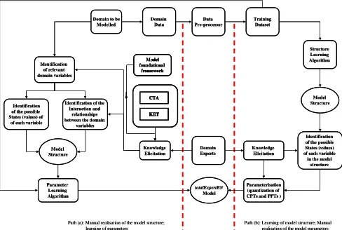
The semi data-centred approach, which scenario is depicted graphically in Fig. 4, entails the use of domain data and the limited involvement of domain expert(s). Fig. 4 highlights two different possible paths, (a) and (b), of the semiDataBN approach. Path (a) indicates that it is possible to construct the model structure manually with assistance of domain experts, while the parameters are learnt from data. Path (b) indicates that it is possible to first learn the model structure from existing domain data, while the parameters are derived from knowledge elicited from domain experts. For both paths, the structure and parameter learning processes described earlier apply.

III. EXPERIMENTAL PROCEDURE

This investigation entailed the construction of several BN models using the three different construction approaches. The total expert-centred model was constructed first, with the committed participation of three domain experts (down from the initial nine from the start of the research work). The foundational framework of the model was anchored on Psychology of Learning, which is focused on understanding how the learning process (often depicted as learning theories and models) works and the effect of learning on behaviour. Learning theories and models are ideas about how learning may happen (conceptualization of the learning process), and are meant to be applied in the instructional process, in order to facilitate learning by instruction and assessment [18]. Assessment drives learning [18]. The framework (depicted graphically in Fig. 5) is consistent with the definition of assessment, by [18], as a generic term for a set of processes that measure the outcomes of learning, in terms of knowledge acquired, understanding developed and abilities/skills gained, because of the intended application domain of the model -- undergraduate electronic engineering students' laboratory work performance assessment.

totalExpertBN Model Domain Experts Knowledge

Elicitation

Identification of the Interaction and

relationships between the domain

framework

CTA KET

Training Dataset

Structure Learning Algorithm

Identification of the possible States (values) of each variable in the model

structure Model Structure

Parameterisation (quantization of CPTs and PPTs ) Knowledge Elicitation

Path (a): Manual realisation of the model structure; learning of parameters

Path (b): Learning of model structure; Manual realisation of the model parameters

Domain Data

Data Pre-processor

totalExpertBN Model Domain Experts Knowledge

Elicitation

Identification of the Interaction and

relationships between the domain

framework

CTA KET Model foundational

framework

CTA KET CTA KET

Training Dataset

Structure Learning Algorithm

Identification of the possible States (values) of each variable in the model

structure Model Structure

Parameterisation (quantization of CPTs and PPTs ) Knowledge Elicitation

Path (a): Manual realisation of the model structure; learning of parameters

Path (b): Learning of model structure; Manual realisation of the model parameters

Domain Data

[image:3.595.305.549.332.496.2]

Data Pre-processor

(4)

In order to build on the framework, Cognitive Task Analysis (CTA) technique was used to breakdown each of the three core component variables (Abilities/Skills, Knowledge, and Understanding) of the framework (knowledge, understanding, abilities/skills) into their constituent constructs. Essentially, the CTA process was used to facilitate elicitation of knowledge from domain experts. Descriptions of the core variables, with respect to the performance of laboratory tasks within the context of the domain, were elicited and used to develop the model. As part of the CTA process, laboratory instruction manuals, and laboratory work assignment sheets were reviewed, students undertaking laboratory activities in the traditional laboratory environment were physically observed, in addition to the knowledge elicited from the domain experts. The end product of the CTA process was the structure for the totalExpertBN. The parameters were then derived from the relevant part of the knowledge elicited from the domain experts. The resulting model, totalExpertBN, served as the reference model for the investigation.

Sample domain datasets and a Bayesian network software tool were required for the construction of a total data-centred (totalDataBN) model. There are two possible sources of sample data: domain historical data, and/or empirically generated data. Where data from such sources are not available, which was the case in this context, the alternative is the use of simulated sample data. Often, researchers needing to undertake empirical investigations, with respect to structure and/or parameter learning, create frameworks that would facilitate the generation of the required sample data from the Joint Probability Distribution (JPD) represented by an existing reference model. Along this line, the bare structure (structure minus parameters) of the totalExpertBN was used to generate two sample datasets, one training dataset (TDSMP dataset), and one test dataset, TD. A second training dataset (TDSPP dataset) was generated with the complete (structure plus parameters) totalExpertBN model. This facilitated the construction of two different totalDataBN models: totalDataBNSMP and totalDataBNSPP, using the Bayesian network software tool, Genie [20], Genie is the graphical interface to SMILE [20], a Bayesian inference engine. Genie supports both structure and parameter learning.

Construction of the semiDataBN was based on both paths (a) and (b) of Fig. 4. Two instances of the totalExpertBN model structure was used to construct two semiDataBN models, based on path (a), by learning their parameters using the training datasets, TDSPP and TDSMP, and the Bayesian network software tool, Genie [20].

IV. MODEL EVALUATION

The different types of BN model evaluation studies include: verification, reliability, validation, and performance check. Verification is concerned with knowledge elicitation review, functional verification, and sensitivity analysis. Review and refinement are usually inherent parts of the knowledge elicitation process. Functional verification entails checking that a piece of evidence entered at an evidence node is properly propagated through the network. Sensitivity analysis (SA) is a technique for systematically investigating the effects of variations in inputs on a model’s output. There are two types of SA: sensitivities oriented to evidence (evidence-based analysis) and sensitivities oriented to parameters (parameter-based analysis) [21]. Evidence-based analysis determines the variables that have the highest or lowest impact on the belief estimation of a target variable, X, while parameter-based analysis measures the impact of changes in the parameters of a node, A, on the probability distribution of a target node, X. Often, only one of these two types of analysis, mostly evidence-based analysis, is employed in any one study,. Verification study affords opportunities for bias minimization in the elicited knowledge. Reliability and validity studies are most appropriate for models geared towards the evaluation of students' assessment scenarios. Performance checks, which are of interest in this context, give a picture of a model in terms of its success rate, accuracy, and failure rate.

Performance verification studies often entail the use of a test dataset, from which a select set of variables from each record instance constitute evidential variable and their values the findings with which to update the model. The remaining set of variables from the same record instance constitutes the target nodes and their values the known observations, with respect to the finding. The test procedure consists of entering evidence at the set of selected evidence nodes of a model, and querying the target nodes. For each network update, for each record instance in the test dataset, the probability distributions of the target nodes are recorded and their predictions determined. That is, after each network update, the state of each target node with higher belief value (the most likely or maximum likelihood state), based on a cut-off threshold probability, is taken to be the prediction for the target node. For example, for a 50% cut-off threshold probability, the state which belief level is higher than 50% is taken to be the prediction. The predictions are then compared with the observations. The statistics from the comparison are used to derive values for the performance metrics (optimality criteria), for the model being evaluated. The optimal refers to the model which is best in terms of the adopted optimality criteria [22]. The performance metrics include: error rate, logarithmic (logloss) score, Brier score, and Sensitivity. These metrics are often used together, in any one model evaluation, in order to facilitate the drawing of more robust conclusions.

The error rate (failure rate) function is based on the maximum likelihood state of the target node [23]. It gives the percentage of the cases in a test dataset for which the query node was wrongly predicted. The logarithmic (logloss) score, suggested by [24], is defined as follows: let X denote a discrete random variable, with m (mutually exclusive) possible states, x1, x2,…, xm, which is to be

observed for a sequence of cases, i = 1,…….,N. Let P(xi)

Improved Performance

Learning (indicates) Knowledge Abilities/Skills

(result in)

Understanding

(result in) (result in)

Improved Performance

Learning (indicates) Knowledge Abilities/Skills

(result in)

Understanding

[image:4.595.90.250.47.182.2]

(result in) (result in)

(5)

denote the estimated probability (referred to as the predicted value for the purposes of the test) for the ith state. Suppose the jth state is actually observed, then the particular observation is associated with a logloss score for the jth state given by [24] as: llll _j =log(1 P x( _j))= −logP x( _j)_.

Then, by accumulating the scores for the N cases, a total penalty value is obtained as:

1 N

j

=

∑

=

l

_{, and the average}

logloss score for the N cases is:

1 1

log ( )

1 1

N N

P x

avg _N j _N j

j j

= ∑ = ∑ −

= =

l l

l l _{. The logloss value}

lies in the range [0, ∞], where smaller (lower) values of the score imply better model performance.

The Brier score (b), also referred to as Quadratic Loss (QL) or Mean Squared Error of Prediction (MSEP), measures the accuracy of a set of probability assessments. The Brier score function, as used in BN model performance comparison, is given by [10][11][28][24] as:

(

)

1 ₂

1 2

(

|

)

(

|

)

1

1 N

k

b

P y

c x

_i

P y

j x

_i

N i

j

=

∑

− ×

=

+

∑

=

























,

where_{P y c xi}( = | ) is the probability predicted for the actual (observed) state,

c

, of the target variable, y (the state of y in the particular record of the test dataset), given the evidence variables, _{xi ; (}p y=_{j xi}| )is the probability predicted for the jth state of y, given the evidence variables; k is the number of states of the target variable, y; N is the number of records in the test dataset. The QL is a measure of the average quadratic loss that occurred on each instance in the test dataset. It is averaged over all the records in the test dataset and not only accounts for the probability assigned to the actual (observed) state, but also the probabilities assigned to the other possible states of y. The value of Brier score lies in the range [0, 1], with b = 0 indicating highest prediction accuracy, thus better performance.

Sensitivity (recall rate) gives the proportion (in %) of actual observations which are correctly predicted. A sensitivity of 100% means that the model correctly predicted all actual observations for the target variables.

V. RESULTS AND DISCUSSION

For the investigation, a total of five different models were actually constructed, where the intention had been to construct seven. The reason for this short fall will later become evident. The constructed models are: the totalExpertBN, two totalDataBN, and three semiDataBN. The sizes of the training and tests datasets were 137024 and 7000 samples, respectively. Two different training datasets (TDSMP and TDSPP – both the same size) and one test dataset, TD, were used. The TDSPP dataset was generated with the complete (structure plus parameters) totalExpertBN model, while the TDSMP dataset was generated with only the model structure (structure minus parameters) of the totalExpertBN, with the assumption of observability. It was also assumed that the data samples are representative of the larger set of baselines samples. The test dataset was used for evaluating the models. The results of the empirical

investigation are hereby presented with respect to the models’ performance metric values and performance indices, shown in Table 1 and Fig. 5, respectively. The performance

index function is given as:

[

(100 e) (1 b) *100 s (1 l) *100

]

normalized(0 1scale)

ψ= − + − + + − ₋ ,

where e = error rate, b = brier score, l = logloss, and s = sensitivity. The function assumes equal importance for all the metrics, taking as input, the values of the metrics, for a model, and yields a performance index for the model.

The results of the investigation, shown in Table I and Fig. 6, are encouraging and highlight some interesting themes. Also, they constitute significant contributions to literature on Bayesian networks model construction. The results, in addition, highlight an important issue for further investigation. First, the performances of the semi data-centred models, semiDataBNSPPa and semiDataBNSPPb, constructed with the TDSPP training dataset were comparable to the performance of the reference model, totalExpertBN. So also was the performance of the total data-centred model, totalDataBNSPPb, constructed with the

TDSPP training dataset. Second, the performance of the semi data-centred model, semiDataBNSMPa, constructed with the TDSMP training dataset, was relatively poor compared to the performance of the reference model, taking 0.50 index as the threshold between comparable and poor performance. Its learnt CPT entries were more or less inconclusive. Third, in all cases where the training dataset, TDSMP, was to be used for model construction involving structure learning (as in the cases of constructing the totalDataBNSMP and semiDataBNSMPb), no structures were learnt. That is, the structure learning algorithm failed to discover any relationship between the variables in the training dataset. This is why there are no performance metric value entries for the models in Table 1. Hence, only five models were constructed, instead of the intended seven. Finally, the totalExpertBN and the semiDataBNSPPb had the highest Performance Index (PI) of 1, followed by the

0.00 0.20 0.40 0.60 0.80 1.00 1.20

totalExp ertBN

totalData BNSPP

semiDataBN SMPa

semiDat aBNSPP

a semiDat

aBNSPP b

Model

P

e

rf

o

rm

a

n

c

e

I

n

d

e

x

Fig. 6. Performance indices of the models TABLE I

PERFORMANCE EVALUATION RESULTS

74.65 0.374

0.5454 29.54

semiDataBNSPPb

71.03 0.3735 0.5444 29.33

semiDataBNSPPa

* *

* * semiDataBNSMPb

46.09 0.4998 0.693 55.06 semiDataBNSMPa

Semi Data Centred

* *

* * totalDataBNSMP

66.69 0.3741 0.5456 29.46

totalDataBNSPP Total Data

Centred

74.65 0.374

0.5454 29.54

ExpertBN Total Expert

Centred

Sensitivity Brier

Score Logloss Error Rate Model

Approach

74.65 0.374

0.5454 29.54

semiDataBNSPPb

71.03 0.3735 0.5444 29.33

semiDataBNSPPa

* *

* * semiDataBNSMPb

46.09 0.4998 0.693 55.06 semiDataBNSMPa

Semi Data Centred

* *

* * totalDataBNSMP

66.69 0.3741 0.5456 29.46

totalDataBNSPP Total Data

Centred

74.65 0.374

0.5454 29.54

ExpertBN Total Expert

Centred

Sensitivity Brier

Score Logloss Error Rate Model

(6)

semiDataBNSPPa with a PI of 0.96, and then talDataBNSPP, with a PI of 0.90. The performances of the three data related models, semiDataBNSPPb, semiDataBNSPPa, and totalDataBNSPP are significant. However, the results indicate that it may not have been possible to construct the three models without first constructing the complete reference model (structure + parameters) (the totalExpertBN model), with the assistance of domain experts. It was observed, as shown by the results, that a complete reference model (that is knowledge of the relationship between the domain variables and their Conditional Probability Distributions (CPDs)) is a requirement for simulating sample datasets for structure and/or parameter that will yield meaningful and comparable models. This highlights the need for further investigation of the effect of historical domain training data samples, not generated with knowledge of the relationship between the domain variables and their CPDs, on structure and parameter learning.

VI. CONCLUSION

The optimal approach for the construction of a BN model for the performance assessment of undergraduate electronic engineering students’ laboratory work in a virtual laboratory environment has been investigated. The exercise has yielded significant results and highlighted an aspect requiring further investigation. The results provide reassurance that the procedure followed in the derivation of the assessment model was fit for purpose. In addition, the results provide additional insight for researchers, and shows that the data- and semi-centred BN model construction approaches depend on the availability of appropriate sample training datasets. The source of the training dataset could impact on the outcome of the model construction.

REFERENCES

[1] M. J. Druzdzel and H. A. Simon, "Causality in Bayesian Belief Networks", Proceedings of the Conference on Uncertainty in Artificial Intelligence, 2006, pp. 3-11.

[2] Wikipedia, "Subject-matter expert", 1 Nov, 2011, http://en.wikipedia.org/wiki/Domain_expert. Accessed 28/01/2012 [3] N. Fenton and M. Neil, "Comment: Expert Elicitation for Reliable

System Design", Statistical Science, vol. 21, no. 4, 2006, pp. 451 – 453.

[4] M. J. Druzdzel and A. Onisko, "Are Bayesian Networks Sensitive to Precision of Their Parameters?", Intelligent Information Systems, 2008, pp. 35 – 44. Accessed March 10, 2011

[5] P. Myllymaki, "Advantages of Bayesian Networks in Data Mining and Knowledge Discovery", 2010. http://www.bayesit.com/docs/advantages.html. Accessed Dec. 12, 2010

[6] R. Rajabally, P. Sen, S. Whittle, and J. Dalton, "Aids to Bayesian Belief Network Construction", Proceedings of the 2nd_{International}

IEEE Conference on Intelligent Systems, vol. 2, 2004, pp. 457 – 461. [7] B. Das, "Generating Conditional Probabilities for Bayesian Networks: Easing the Knowledge Acquisition Problem", August 4, 2008. http://arxiv.org/ftp/cs/papers/0411/0411034.pdf Accessed Feb. 24, 2010

[8] M. J., Druzdzel, & L. C. van der Gaag, "Building Probabilistic Networks: Where Do the Numbers Come from?", (Guest Editors’ Introduction). IEEE Transactions on Knowledge and Data Engineering, 2000, vol. 12, no. 4, pp. 1-485.

[9] K. Ng and B. Abramson, "Consensus Diagnosis: A Simulation Study", IEEE Trans on Systems, Man, and Cybernetics, vol. 22, no. 5, 1992, pp. 916 – 928.

[10] R. G. Cowell, "Parameter Learning from Incomplete Data for Bayesian Networks", 1999a. Retrieved from http://www.staff.city.ac.uk/~rgc/webpages/aistats99.pdf. Accessed 03/07/2009

[11] L. Oteniya, "Bayesian belief networks for dementia diagnosis and other applications: a comparison of hand-crafting and construction using a novel data driven technique", Unpublished PhD Thesis, Department of Computing Science, University of Stirling, Stirling, FK9 4LA, Scotland

[12] D. M. Chickering, D. Geiger, and D. Heckerman, "Learning Bayesian Networks: Search Methods and Experimental Results", 1995. Retrieved from http://research.microsoft.com/en-us/um/people/dmax/publications/aistats95.pdf

[13] G. F. Cooper, "A Bayesian Method for Learning Belief Networks that Contain Hidden Variables", AAAI Technical Report WS-93-02,

1993. Retrieved from

http://www.aaai.org/Papers/Workshops/1993/WS-93-02/WS93-02-011.pdf

[14] M. Forster, and E. Sober, "AIC Scores as Evidence – a Bayesian Interpretation", 2010. Retrieved from http://philosophy.wisc.edu/sober/forster%20and%20sober%20AIC% 20Scores%20as%20Evidence%20jan%2028%202010.pdf

[15] D. M. Chickering, D. Geiger, and D. Heckerman, "Learning Bayesian networks is np-hard", Technical Report MSR-TR-94-17, Microsoft Research, November, 1994. Retrieved on July 22, 2010 from http://research.microsoft.com/apps/pubs/default.aspx?id=69598. [16] R. W. Robinson, "Counting labelled acyclic digraphs", 1973. In F.

Harary (Ed.), New Directions in the Theory of Graphs, New York: Academic Press, pp. 239-273.

[17] G. Heinrich, "Parameter estimation for text analysis", Technical Note Version 2.4, August 2008, vsonix GmbH and University of Leipzig.

http://www.arbylon.net/publications/text-est.pdf. Accessed 19/07/2010.

[18] W.L. Neuman, Social Research Methods: Qualitative and Quantitative Approaches. 2000, USA: Allyn & Bacon. In H. Page-Bucci, "The value of Likert scales in measuring attitudes of online

learners", February 2003.

http://www.hkadesigns.co.uk/websites/msc/reme/likert.htm. Accessed 26/01/2011.

[19] QAA (Quality Assurance Agency), (2006). Code of Practice Section 6: Assessment of Students. Retrieved February 3, 2008, from the QAA

website:http://www.qaa.ac.uk/academicinfrastructure/codeOfPractice /section6/default.asp

[20] M. J. Druzdzel, "GeNIe: A development environment for graphical decision-analytic models", Proceedings of the Annual Symposium of the American Medical Informatics Association, Washington, D.C., 1999, pp. 1206. http://www.pitt.edu/~druzdzel/psfiles/amia99.pdf. [21] J. Jordana, and F. J. Sànchez, "Cooperative work and continuous

assessment in an Electronic Systems laboratory course in a Telecommunication Engineering degree", Proceedings of the 2010 IEEE Conference on Engineering Education (EDUCON), 14-16 April 2010, Madrid, 395 – 400.

[22] L. A. Zadeh, "What is Optimal?", IRE Transactions on Information Theory, 1958, pp. 3.

[23] NSC (Norsys Software Corp), Netica-J Reference Manual (Version 3.25), 2008. http://www.norsys.com/netica-j/docs/NeticaJ_Man.pdf [24] I. J. Good, "Rational decisions", Journal of the Royal Statistical

Society, vol. 14, 1952, pp. 107-114. In M. Roulston, "The Logarithmic Scoring Rule a.k.a. “ignorance”", Retrieved from http://www.cawcr.gov.au/bmrc/wefor/staff/eee/verif/Ignorance.html [25] R. Cowell, "Probabilistic networks and expert systems",

Springer,1999b

,

[26] F. V. Jenson, Bayesian Networks and Decision Graphs. Springer, USA, 2001.

[27] M. S. Roulston and L. A. Smith, "Evaluating probabilistic forecasts using information theory", Monthly Weather Review, vol. 130, 2002, pp. 1653-1660.

[28] P. Doshi, L. Greenwald, and J. Clarke, "Towards Effective Structure Learning for Large Bayesian Networks", AAAI Technical Report

WS-02-14, 2002. Retrieved from