The dynamic behaviour of packed distillation columns

THE

DYNAMIC BEHAVIOUR Of

PACKED DISTILLATION COLUMNS

A thesis pr~sent~d for the degree of Doctor of Philosophy in Chemical [nqineering

at tile

University of Cailterbm·y, Christchurch, New Zealand.

By

P ,, '-1 • JORDI\N

ENGINEERING LIBRARY

AC K N 0\•Jl,F. DGI·:t•11·: N TS

I would like to thAnk Dr. ',v.B.Earl for his supervision of this project and for the practical advise which he was able to offer. Thanks are also due to the technical st~ff of the Chemical Enqineering Department for their help with modifications to the experimental column.

This project wotlld probably never have reached completion without the support of Professor A.N,Kennedy, with his sympathetic understandjng of the problems of members of staff doinq Ph~D work, and the unfailing encouragement of. 1ny wife Erica durinq the. lonq days of her "Ph.D w .i rlowhood 11_•

Financial help from I.C.I. (N.Z.)Ltd. is gratefullY acknowledged.

This thesis was formatted usinq a computer program written by

G.F.Deecknr of the Computer Science Department, For his help, and that ot the Computer Centre Staff, especially G.Gregg of Lincoln College, I am

ERRATA.

1. Page 20, first line after equation (2.14):

Change "where XB is the equilibrium composition" to "where XB is the liquid composition"

2. Page 32, equation (4.1):

Change "z(z,o)" to "x(z,o)"

3. Page 34, second line after equation (2.4) Change "(L/Z) (Clx/Clt)" to "(L/Z) (Clx/Clz)" 4. Page 64, para 2, line 4~

Change "This is about 5%" to "This is about 2.5%" 5. Page 77, second to last line:

Change "0.025 mV" to "0.0025 mV" 6. Page 87, para 1, line 1:

Insert "I" in the list: "At thermocouples D, E, H, J and L." 7. Page 106, equation (8.3):

Change "Lox" to "Lox"

az

zaz

ADDENDA.

[; m·,

~II\ RY,

CliAP'fER 1 :

CHAPTF.H 2:

Cll.'\PTER 3:

Cllt\P'rl'.:R 4: CHAPTER 5:

CH1\PTEH 6:

CHAPTER 7:

CHJ\P'l.'EH 8:

CH1\P'l'8R 9:

.snmor,s.

·m:F E: H ENCES •

APPENDIX J. :

AFPUI::JIX c, •

,;

.

APPENDIX :3 :

APPENDIX 4: APPENDIX 5!

CONTENTS

Introduct1.on.

Dynamic Model of a Packed Distillation Column, Numerical Solution of the Model,

Results of the Computer Solution of the Model. Modifications to the Model for Other Column 1\rrangement s.

The Experimental Column and Mixture. ExperimentAl Composition Profiles at

St~~ady SU1te.

2:2

31

42

82

ExperimentAl Composition Profiles at 94 Unsteady State.

Conclusions and Suggestions for Further Work. 110

Fnthalpy Balance in the Packing, Computer Subroutines,

Computer Mainline Program. Operating Variables.

Transient Response Plots.

116 1?.0

'l 2?.

123

13 4

The dynamic behavio11r of packed distillation columns separating binary mixtures has been studied, both by means of a computer siwulation, and by experimental testin~ of a column.

The numerical solution of the partial differential equations of the mathematical model, obtained using a diqital computer, was eound to be fnst, accurate and stahle. The advantages obtained by usinq this approach, compared With previous analytical solutions, included: no restriction on the equilibrium relationship which could be used, variable coefficients could he used Jn the partial dif~erential equations, Rnd the method allowed any desired botlndary conditions to be used, The model was first solved for an enricl1inq colu~n section, and was later extended to the cases of batch and continuous columns.

!I -l 50 rn m d i arne t e r. UJ lll nm p a c 1<; e d 1·1 i t h t 0 m m ll as c h i 9 r i n g s ~w s u sed

CllAPTER 1 IN'l'HODUC'l'lON

1.1 The Scope Of This Work. 1.2 Applications.

1.3 Previous Work On Packed Distillation Column Dynamics.

1. 3. 1 1 '3. 2 1. 3. 3

1. 3. 4

Previous Models. Assumptions Made.

'l' he a l. m of h i s s t u d <"Is to use n urn e r 1 c a 1 solution tech n 1 s to s o 1 v e t.l1 e d y n a m i c m o d <' 1 o f ,, p ·"~ c k e d d l s t i l l a t i o n c o 1 u fi1n , a n d t o o b Ud n experimental mensurements to test the effectiveness of the model in predicting the dynamic behavtour of a real column,

rt

was restricted to ttle study oE columns separating binary mixtures .•

The work falls into two parts. In charters 1 to 5, the work of previous investiqators on Packed distillation column dynamics is first considered. Then the dynamic column model is presented in a form suitable for solution on a digital computer. Typical results are presented and It is shown that when a numeric~l solution is used, the model may be easilY adapted for different column configurations hY changing the boundary conditions.

The experlmentRl column is described

ln

chapter 6; Experimental results are ~rese~ted for the column at steady state (chapter 7) and unsteady state (chapter 8). Chapter 9 summarises the effectiveness of the model in predicting the dynamic response of the experimeJltal column to upsets io retlux ratio, and attempts to p.iproint those aspects wl11cl1 require better understandinq before the performance of the model can be

.1 mproved.

1.2 APPLICATIONS

A distillation column can be considered to be in a dynamic condition i f any variable in the column (e.q. corr.posltion rwldup or flowrate) is changlnq with tlme. Otherwise the column ls at steRrly state. There ore three m~in situ~tions in which knowledge of the rlynam1c

4

( .l) • II a t c h d i s t i l 1 ,1 tJ on , Cor:~ p o s It i on :; tiH o u q l )() u t .:1 co lu rn n , con U n u a tl y

descriptions of batch rlistill~tion, e,q, Boqnrt(I9J1) and nose and Wclshans(1940), ianore the effect of column holduo. They therefore trent the column composition profile ~s belnq at steady state at AllY time, but with a time varying boundary condition (the reboiler composition), for a

review of batch distillation models see Kropholler et. al,(l968),

Cii). Automatic control. Most industrial columns have some form of au tom a tic prod tl c t con t r o 1 , of. ten A c 11 i eve d by rna n 1 pula tJ. n q t 11 e ret lli x ratio. In the design of such control loops by classical methods, the column must be represented l1y transfer functions; either empirical or

d e r i v e d f r om a d y n a rn 1 c m o d e 1 o f . t 11 e c o 1 u m n • A r e v 1 e w o f t h e u s e o .t p 1 a t e

rlistlllation column models in control is given by Posenbrock(1962).

(iii), Column startup, :columns are often started at total reflux and then switched to the operatinq reflux rate. The time taken to achieve steady state at total reflux in some situations may be so long that it

cannot be lqnored, especially in batct1 operations, Cohen(191\0) has

reported startup times of many days for columns separatinq isotopes bY distillation •

1 , 3 PREVIOUS WfJHl\ ON P i\C Kr::D II I ST I LLl\ T I ON COLU~HI D YN AIHCS •

Investiqation of the dynamic response of binary packed distillation columns has been reported by: Cohen(1940), Bowman and

Hria~t(1§47), Marshall and Piqf;rd(1948j, Jawion-and ~mith(1954), Heinke

et, al. (1966), Heinke and \·1 n CT n e r ( 1 9 6 5 ) , Kropholler et. A1,(1968), Tomassi anrl Rice(t970), Borchardt and Wagner (1971), and Kuznik and Krzyzanowski(1975). Of these, lleinl<e et. al. 1 Krooholler et, al. ,

s e v c n~ l h o r s l n c d 1 n i\ r c 11 c r <~ n d H o h t u s ( 1 9 6 1 ) , H s en b rock ( 1 r)(> 'I ) <HHl

':i 1 1 1 1 i) 01 s ( 1 9 6 3 ) • T 11 c rJ y n 'l r:1 1 c s of: o t h C! r t y P c s o f p d c l< r. d co lu r"· n s ~ t1 c h as packed absorption columns ha~ been considr.retl bY Jawson and Smilh(1054).

1. J. 1 Pre v i o u s f. I ode 1 s ,

In the works on packed distillation column dynamics cited above, the mathematical model has been derived by considering mass balances for the more volatile component ln the liquid and vapour phases over a small element of pocking he.i.gllt. Thesf~ yteld equatlons of the form:

where: H ll

L

v

X

v

t

1

n

(~

N

::: 1.ax - N

-- a·7

::l.tquirl l!oldup :::vapour holdup =liquid flow rate =vapour flow rate

-=rnole fraction of. more volatile component in the liquid phase

=mole fraction of more volatile component in the vapour phase

=time

=he 1 gl1 t from bottom of packlng

:::total P<lCkinq he.tqht =mass transfer rate

The mass transfer rt1te t(~rm N ls usu,1lly expressed as:

*

N - K a.S(y -y)

•••• ,(1.1)

••••• (1,2)

mollm mol/m molls molls

s m

m

rno.l./m/s

or:

.j<

N .. K n,S(X->X

L

X c~equ.ilibrJ.um n10le traction of the more volatile component in the liquid

*

y =e~uilihrium mole fraction of the more

K

a G

s

volatile component in the vapour

=overall mass transfer coefficient times interfacial area

~overall mass tjansfer coefficient times interfacial area

=cross sectional area of column

•• , , , (I, 4)

3

rnol/s/m

3

molls/rn

2

m

6

equations 1,1 and 1.2 are hyperbolic partial differential ~quations and. are, in general, non-linear.

7

1.3,?. A s s u n1 p t i o n s 1·1 a d e •

T l1 e f o 1 1 ow .I n g '' s s urn p t1 on s were m ,vl e by a l.l <J t 1 t. h o r s c it· 0 d above t n

writing and solving the mathemAtical model:

(1) constant molal l!qul.d and vapour flow r.:1tes tll'couqhout nny packing section,

( 1 i) constant liquid and vapour holdups throuqhout any racking secU.on,

( i 11) no radial variation in liqu.id or VApour composition,

(iV) no ax.ial dispersion in either phase. Kropholler et, al.(i968) investigated the eff0cts of axial dispersion in both liquid and vapour phases, but found that their steady state e~perimental

results were best fitted when axial dispersion was ignored,

(V) the mass transfer riltc is described by ettller equatl.on (1.3) or equation (1.4). Rowman and BriantC1947) discuss various mass transfer mechan.lsms b11t use those just mentioned in solvinq the dynamic case.

(Vi) the mass transfer coefficient is constant throughotlt the column.

1'•1ost workers also assurned that:

(vi 1) t 1) ere 1 s <> l.i near e q u i l i. b r 1. u m r e 1 at ions hi p ,

*

I.e.

y

=

m.x

t

c

*

or

X :: rn.y

+

c

where m and c are constants.

Exceptlons to this were CohenC1940l, Borchardt and \'!aqner (1971), and Heinke and Wagner(l9fi5), who used a P~oult's Law relationship (i.e. constant relr:1t1vc volatility), althouqh the latter authors then 11neariscd thls in the operating reylon.

( v 1i 1 ) t h t' r e 1 s n o v ilP o llr l\ o l d up , ill t110 u q h t h e

v

d o n o t s t:.H c t h t s , To rP a s s i and P 1 c 0. r:1ll s t t1 "' v e il s s llln e d 1'. ,, r o t i n u i. d !1 o l d up .! n il r r i v l n q

il t P. q U cl t i 0 fl .S ( 6 ) MH) ( 7) J n t h C f r r i1 p C t' J 0 tlH' r\\'[ S P. t h l' r (> W 0 U .l d b 0.

o axlatheta term in e~uatlon (6).

Ox) the con1postt.tons ut tiH~ tJni'll steady stote ,ue known in advance.

I I r: ink e and \·I ,vm e r use l< now 1 e d <1 e of the f in a l s t e '" d y s tat ~~ to . .U near 1 s e t: heir e q u 111 b r i u m r e l a t.t on s 111 p, To r:h'! s s 1 and

n

1 c e use the initial and final compositions at the top and bottom of the

co 1 tlmn to fit their equilibrium curve before the Initial

con1pos.tt.ton profile or the transient resronse can be co1nputed.

The following assumptions have usuallY been made conc~rning

boundary conditions:

(x) there is zero condenser holdup. This means that the llauid and vapour compositions at the top of the packing are equal.

(Xi)

I.e. y(Z1t)

=

X(Z,t)

Kropholler et, al,(196R) ~llow for the introduction of condenser time constants. Bowman and Rriant(1947) d.tscuss various po5sible boundary conditions while Marshall and Ptqford(1948J do not insert any into their Laplace Transformed equations.

there is infinite reboiler holdup. Alternative expressions of the same condition are thAt the reboiler composition

is

constant, or that the vapour composition enterlng the bottom of the packinq is constant.

Jaw~on and ~~itht1954) postui~te that a disco~tln~if~ in an

operatlnq parameter Csoch as llt1Uld reflux rate) will cause <1 numb(~!" of succeedinq discontinuities in liquid composition proceedin<:J ~Jo•t~n t11e column, and in vapour cowrosition oroceeding un the column. This has not b e e n r e p o r t e d by t h o s e A 11 tt1 o r s q u o t e d 1 n s e c t1 o n C I • .1 ) a s t1 a v i n q cl on e

1. 3. 3 ~io1ution

or:

'The I::quat.!.ons.

Those authors who h~va obtained solutions for the trilnS!Pnt response of,) p<Jcl<ed clistilLli:i<)n col\lf'ln from the maUH•matlcol 1r.odel tHlVl' done so u;;inq ,,nalytical r1(:thods. T II e m c1 j o r l t y tvw e rna d e u s e o f t li e Laplace TrAnsforrn method, Kropholler et, al.(1968) say thC\t th<~Y have solved .the equations numerJcalty, but that their numerical solution took several hours to evAluate compared with seconds for the analytical solution. The analytical solution is usually presented ns the sum of c1 series of exponential terms; the experimental results of Heinke et, ul, (1966), Tornassi and RJce(1970) and Kropt1oller et. al. show that the first two terms are usually SIJfficient to characterise a transient response • X r o p 110 11 e r e t • a 1 • p o 1 n t out t h a t the ' t i me cons tan t s ' are the same for differing dynamic conditions, e,g, the response to upsets in liquid reflux or entering vapour rate or composition, and for the approach to equilibrium ~t total reflux after initial warming up. Borchardt and ~agner (1971) used a semi-empirical method to c&mpute the

'ti~e constants' from the steady state composition profiies, The term

'time constant' is not strictly applicable to a distributed parameter system such as a packed distillation column.

To o b t a 1 n an a 1 y t i c a 1 sol u t ions o £ the mode 11

i

t h d s been til' c c s sa r y

to have constant coeffict~?nts in equations ( L t ) and (1.2). This has required the as~umotion of constant flow rates, holdups and mass transfer coefficient in the coJ.umn as menUoned in the previous sect:ton,

also been necessary to use a linear equilibrium relationship over the whole corni,osi tion in the column, or, 1\uznll< find

Yr~yzanowski(1~7~) h~ve do0e, to use linear approximatlOQS to the eouilibrium curve over a number of segments. As Kropholler et. al, have rernarl<ed, some of the an<~lytical solutions, notably those of ,];1wson and

'10 Pre V tOilS E:q•e r I '"<<'n td l Pes 1.11 t s,.

He 1 n k e e t • a 1 • , K r o ph o ll t.' r e t , a 1 • , Ton, :1 s s .l and n 1 c c , d n d Boy 1 t~

Palmer(1973) have publ.lshed experimental clynnrnic resnonst:"! measurements made on packed distillation columns.

Heinke et. al. (1966) measured the dynamic response of a p[tcked

distillation column to step chan<res .in the liquid reflux rate larqe enough to cause larqe changes in composition, thus making the assumption of a linear equilibrium relationshiP poor. Their column was 75 mm in diameter, 3.9 m hlqh and packed with 4 mm glass Raschig rings. The column wall was heated to maintain adiabatic operation. The test mixture tlSed was benzene and trichloroethylene. The distillate WRS returned to the still to maintain an almost constant rehoiler composition. The composition was me~sured at the top of the packing and at three intermediate levels by withdrawing a liquid stream and using a dielectric constant analyser.

The co~posltion transient responses were presented mainly dS graphs of loq(<ievlation from final steady state) versus time, On these plots, all lines for a given transient run became parallel straigl1t lines after some time. The authors concerned themselves mainly with the approach to_the final steady state and the 'time constants' obtained from these plots. They found that the dominant 'tlme constant' was the same at each level tor a qiven final steady state and did not depend on the initial steady state. This was in agreement with the solutions of the model obtained hy other workers using a linear equilibrium rel~tlonship,

The response w~~_found to be fDster tor decreasing reiltlX ratio between a 0iven pair of steady states than tor incre~sing reflux ratio between the same steDdY stntes. no qu,Jntitutive comoarison w,1s made between the experimental results and the predictions ot a ~athematical model.

K r o ph o 1 .l e r e t • c1l , ( 1 q 6 8 ) tl sed a co 1 u :n n 11 1 n c he s t n d 1 a _fl' e t e r w J t h a

r " t 1 o was s t u d i e d ,l n rl a q a i n Ill' d I s t t.l l t e s r P t u r JW d cl .t r c c t 1 y t o t lv~

still. T h e 1 i q u 1 d c o 1r p o s i t I o n '>~ t.1 s rn c cl s u r c d o n l y ,, t t h (' c o .t u r~ n h e -:1 d ,, n d

b,3se and tn the :>till usinq an on--llne oas liquid chromatoqraph, The equilibrium relationship over a wiclc composition ranqc,

responses of the top composition for three chanqes in liquid reflux rate are presented in the parer, and the agreement between experimental and predicted compositions is excellent. However, no indication is qfvpn of the actual composition chanqes or how the holdups were estimatccl, In predictinq the response, the value of K a for the final l.iquid rate was

L

used throuqhout the transient response and any dependence on composition

11 .:1 s i g no r e d •

1'ornassi and Rice(1970) used ethanol~water .tn a fiO rnrn diar.1eter column with 4 sections 300 mm high packed with 4mm cerDmic Her! saddles. They also measured the tesponse to step chanaes in the liquid reflux rate witl1 the top product returned to the still. The composition \'.'2tS measured

at the end of each packing section by withdrawing s~moles and measuring refractive index or density. Tof!1assi and Pice found that their major 'time constants' were independent of heiqht except for the one run done decreasing ratio. They forced· the predicted final compositions at the top and bottom of the packing to match their experimental values by using these to compute the coefficients in their linear eq11Llibrium relationship. The predicted and experi~ental final compositions at the intermediate levels then agreed well. For most .of the six runs tr)ere was good a(Heement between Uw predicted and experimental unsteady state co~positions, especiallY at the top of the packing. However for the run Nith_decreasing liquid reflux rate, the predictions were very poor for the initial part of the run, and at the two top levels moved inlti~l lY in the wrong direction. by a significant ,,mount. Tomassi and Pic·: say that in all cases 'thr reriods predicted fot the change in concentr. 1_{on to rPach 95~ of its equilihr!um values}

dre accuri.lte'. ~~ 1 t h o u q h · (l P. 9 'j 'li r e s p on s e t 1 rn e rn a y h e a q o o d c r 1 t e r 1 on f o r t h e 5 t u tl y o f t h e a p p r o ,, '·· : . n f: a c o 1 u 111 n t o s t e a d y s t d t EJ o n s t.'J r t u p , t o r

'j ?.

qua 1 1 t y o t i:l p r P d i c t t on , 1\ n1 o ck l v: h i c h n1 d y s o rP f' t ( rn 1:' ~; p r e c1 i c t t tH1 t t he 1n1tinl chanqe in co~rnsitlnn is in the opposite clirectlon to the reill sitUation COUld CdUSC SPrlous problems in the onuline control Of a column.

'A 11 these 'do r% e r s have he en concern e cl m .:ll n 1. y w t t h est a b 11 s h in q tl1 G size of tl1e mc1jor 'time constants 1

which control the approach to the new steady state conditions. ·However 1 in automatic control si tuat.ions

especially, the prediction of the earlY part of the response to an upset may be of more importance. None of them have proposed a suitable criterion tor assessing how well a mathematical model pertorns in predicting the behaviour of a real column.

1·\eusurements of the dyn,lrnic beh,3Viour of a packed distillation column have also been reported by Boyle and PalmerC1973) who used a column 3,1 fe~t l)igh and 6 inclws in didmeter to test the metl1ocl of using

pseudo~random binary siqnals for obtnlning the frequency response of a process. T h t~ tr e q u e n c y r e s p o n s e o f t h e t o p c o 11' p o s 1 t1 o n o E t.!1 e i r continuously operating column was found for disturbances in the liquid reflux rate, and the results were compared with frequency responses obtained by step testing and sine wave testing .• The llqulrl compositions were found by measttrlnq the temperature of the binary system. The authors we~e interested in the use of system identification methods rather than in the dynamics of packed distillation columns, and made no attempt to model the column other than by comparing the response with

that of a lumped-parameter first order system.

separate. The requirement of constant coefficients may be satlstiod by

carefully choosiJ)g the binary system to have equal molal latent heats anrl molecular weights, and by operating the column adiabatically. While this may be possible under laboratory conditions, it is obviously impossible that these conditions will all be met in applying the model to many industrial columns.

14

CHAPTER 2 DYNAMIC MODEL

or

A PACKED DISTILLATION COLUMN,

2,1 Introduction

2,2 The Dynamic Mass Balance Equations 2 • .3 Flounclary Conditions

2.3.1 Condenser Boundary Condition

2,3,2 Reboiler Houndary Condition

2.4 Initiill Cond.it.lons

L,J

)"·

i,~

c.

.,J

bJ

1·--·

:5

_,J

:;::.

~

l ·I

J~

(;) C:) t--1

c::l

HOUJUP

2

a

J.

"'"" """•

:)) t•)

,,I _•l

4· ').

:J) H

\ J .,..,

,,

"

l~

r-. ..--.

>

=J

,j <J

·{~ +

"t,..,_

~-..;..; _J

.._.

-z

:.n

"

?. • 1 1 NTIWIHlCT I CHI, 15

Some of: the d r a 1·: b ,~ c k s o f. t h <' pre v 1 o u :> clli d 1 y t i c ,'Jl ~; o l u t l on s o t t

n

e d y n a m i c f~ q u a t1 on s m a y b e a v o i d e d b y t I H.' u s e o t il n u :r~ c r J. c <1 l :; o J \l t.i o n • These have become much more practlcal with the incre<)s~d 511eed of diq(tdl

computers. The advantages of ~ numerical solution are that the

equilibrium relationship may he taKen as any desired non"linear curve, dnd that atw bound<:ny conditions may be used, 'fll•? soJ.utl.oi! is .:11so easily adapted to handle different situations.

In this chapter, the model ~ill be developed for the most simple situation and it will later be extended to handle other cases, The column described by t.lle b,lsic model is shown In fi<J. 2.1.

essentiallY a batch column with the product returned !~mediately to the

still to provide ulrnost constant reboiler holdup and rcbotler

cornpos i tlon, I t is ·~:11e same arranqement as th<lt used by HE.i.nlr:1~

e t • a 1 • ( 1 9 6 6 ) , !< r o ph o 11 e r e t , .::~ l • ( 1 9 6 8 ) an d T o.rr. <:1 s :> i an d lU c e ( 1 'J7 0 ) ,

2,2 THE DYNAMIC NASS BALANCE EQU~TIONS.

~·lass balances for the accumulation ot the more vol3tite component within the liquid and vapour phases over a small increment of coluMn heiqht ~z (see fig, 2.2) Rre given by:

o(H.x) :;;

-~

acL.x) ~ K

a.scy

~y)

--~ .. G

-at

z.az

*

B(h,y) ·· • a(V,y) t K a,S(y •y)

-·--- - - - G

at

z.a-z

••••• (~~1)

••••• (2,2)

pacl<inq, (z::o.o at the bottom ot the Pc:\Ck.tnq dtHI I ,0 CJl the t·()p of. tht~ p [J C k 1 f) g ) 1 <1 f) d ttl e 0 t h C' l' V c1 C J <l b ll' S d r E:' r:l S de f ill C d i 1'1 S (' G t: 1 0 f) \ , 3 , t ,

The ass u m p t l. n n s made in IH 1 t 1 n g e qua t.i on s 2 • 1 and 2 , 2 a r r. t. t1 at

(1) the mass transfer rate is given by K a,S(y -y). Thls is the G

most widely used mass transfer rate expression for packed column mass transfer.

(11) axial dispersion has been ignored.

( i1 i) the dead time following an upset has been ignored. The lonqest

tiwe delaY would be for upsets in the liquid reflux rate to the top of the pacl<!nq, i1S the liquid residence Urre .\s rnuc)) greater than that of the vapour. If the dead time is significant, then the transformation of the time variable to:

t'

=

t - Z(l·z)H/L

could be mC\de. The variable t would then be the total time e 1 a p s e d s l n c e the ups e t on d t ' IV o u .l d · he the ti .rn e s 1 n c e the upset reached height z assuming plug flow. Since dt'/dt

=

1.01 the dynamic mas s b <tl an c e e q \J a t i on s w o ul d be u n c h i1 n g e d by t h i s

trC~nsform<'lt.ion,

It will now be assumed that:

(iv) tl1ere is no rad.tal ·variation of the composition :in either phnse. This assumption is not required for equations 2.1 nnd 2.2 to be valid, provided that x C~nd y are ta~en to be the mean compositions at height z,

The variation of liquid and vapour rate with height may be

co~put~d from an enthalpy balance, t~king acc6uri~ of : (aj heat losses from the column, (b) the difference in the molal latent heats of the binary components, anrl (c) the heat of m!xlnq if this is known. Such an enthalpy balance is rresented in ~ppendix 1.

( v 1)

( v

i1)

the mass trdnsfcr coefficient Is 1nd•~Pendent ot column

position, flo'.'/ rC~t<~ and cornposttion .• The likely varli.ltJ.on in practice \'i .lll be discussed further .tn chapter 6, and experimental values 'll.ill be qiven in chapters 5 and 7.

the liquid holdup and V.-1Pour l1oldup oro constants, In chapter

6, it wl.ll be shown that the liquid holdup can be expected to vary stronqly with liquid composition for the experimental column in this worK, because the two ~omponents used have widely differing molecular weights. The liquid holdup is also expected to depend on liquid rate to the: power ot 0.6, so that tor a chanqe in liquid rate, there W.ill be <1 change in H, The difficulty in predicting the rate of chanqe of ll.qu.id holdup with time, is shown in chapter 8 to be a possible source of major problems in situations where the liquid holdUP changes significantly. The molal vapour holdup wJll be independent of composition for ideal gases and will chanqe veiy little with

\H th these dSS\Hnpt ions .lnc luded, the mass b.:) lance equations

*

Hax :: Lax >J K ii.SCy ~y)

G

at

zaz

*

hay

=

-vay + K

a.s<y

-y)

G

at

zaz

••• ,,(:;Ltl)

••••• (2.5)

The assumptlons made so far are those which have been used by

pre vi o us 1·1 or k e r s ( s e 0 c t1 apt e r 1 ) , No res t r 1 c t1 n <J. ·1 s s urn p t i on s h i'l v e been

·+:

18 analytical function, or an empirical curve fJtted to experimentAl dat~.

*

for convenience, y (X) will be replaced by the symbol f where it Is understood that f is a function of x.

Because the vapour holdup is usuallY small compared with tl)e

liquid holdup, the equations for the case of negligihle vapour holdup

will be developed together with the case for finite va~our holdup. For

h=O, equation (2.5) becomes:

o

=

~vay + K a.SCf-y) ••••• C2.5a)

- G

zaz

The equations are now written as:

-b a y ~ c _{( Y"O :::}

aY ••••• (2,6)

1 - 1

az

at

b ax + c (y-f) :::

ax

••••• (2.7)

2~ 2

az

at

'flhere: b ::: V/(h,Z) ••••• (2.8)

1

c

₌

K a.S/h :::

v.N

/(Z,h) ,. •••• (2,9)

1 ·G OG

b ::: _{L/(H,Z) ••••• (2.10)}

2

c

₌

~~ a,S/H

₌

V,N /(Z,H) ••••• (2.11)

2 G OG

and N

₌

Z/H ::: Z/ (

v

/'r<. a,S) . . . (~.12)

OG ClG G

~ is the number of overall gas-phase transfer units and OG

H is the height of an overall qas-phase transfer unit, OG

... "'>

l!)

J'<.

'I._._..

\!'"U('l vi;)

_, .... ~., .. ,_" '"' '"' ---:_':>·-,,~··-·-"·-•>< ... ,, .. __

!

... "'.'"'•"··-.,

( ", ~->'

(

...

--.,~-

... -.-·r<

I

"'J! c·l' '") h • • - . /

l '· ' . ' ' '\ . '-- .,--)

F ... /1 ',.-I. J t ->~ > ''-~ .c,- ' \ . - ' , \ , , . , - . • •

.-.-·

....

,

..

l ... ~ .,?" " /

s· tt ~ ,,...,.~,. ~~~

.-.,....__,.~.._ ~~-~ ~~' '" .,,..,.,.__,..no-~ • "<' ..,..,..-.~-,....,.'-'-' ~-""'"'-="' --< """"'-".._

.,.)

\I ,,,

/

v~

/ / \

17:)

1 - ... ~

___ _j

'

~:/

~./

t"'"""

1·,:)

"'

··b

av-

c

<v··t.)

-~

o

• ' • " • ( 2 • (J t) )

1---·

az

with b

..

vn

••••• (2,tla)

1

and c

..

I< a.,s

-

v ,,

tJ /Z ••••• (2,9a)

I G OG

Eauations (2.hl ~nd (2.7) arc non•llnear, t~nlictt, hyperbolic, partial differential equations. The numerical solution of suc11 equations is well described by von Rosenberq(1960). Two boundary conditions and two initial con<ll.tion~; are needed before the solution can be computed,

2. 3 BOU ~iDA!<¥ COI\'D IT HlN S,

2 ']. 1 Condenser 8oundary Condition.

The c9mnosition of the liquid returning from the condenser to the top of the column is provided by a mass balance around the condenser

( f i 9 . 2.3),

HC,dxCI ,t)

=

V.y(t,t) • V,x(l,t)

----<:rc-·

•.•••• (2.t3)

where HC is the condenser holdup in moles. The notation y(1,t) means Y at hetght z=l.O and time t. The condenser is thus represented by a first order staqe with constant holdup. If the conrienser holdup is not

co~stant, this eRn easil~ be ~~cou~ted tor by Including a term for x(l 1t),di!C/dt Jn eouation (?..t3). If cles.tred, a deadtirne could also be included by writing the 0qudt1on as

, • , •• (2, 13u)

20 \H1en n1(~ condenser t·lO.tdup is neqliql.ble, PQilation ('2,15) reduces to:

Y(l,t) ·· X(1,t) ••••• C?..13b)

?..3.2 Peboiler Boundary Condition.

The composition of the vapour entering the bottom of the column is taken to be in equilibrium with the liquid in the reboiler.

'rhus y(O,t) -· fCXB) ••••• (2.14)

where XB is the equilibrium composition In the reboiler. If Xll does not change, then y(O,t)

=

canst. If XB changes with time, then XB(t) is found from a mass balance Around the reboiler (fig. 2.11 •

. l_i_R,dX\L:: (V-J,).x(l,t) + L,x(O,t) ~ V.f(XB) dt

where HR is the reboiler holdup ln moles.

2.4 INITIAL CONDITIONS,

•• ,,.(2.15)

H

._! ·I-"

"'

,-1

...,

H

,_,

_.J

I

>

' - '

FIG Za5

STFRDY

[image:27.600.100.416.80.597.2]

2 1

;; t c .1 d y 0 t d t e Co r·1 1:· o s 1 t ion 1:~ 'l 11 d t 1 on s •

The steady state is qivPn by eq\l,ltJ.ons (2,B) and 2,9) wJth the time derivatives set to zero.

I~ e. : ''b dy/dz ~ C (y•af) - 0

I l

and b rJx/dz + c (yyf) -

o

2 '/.

Substituting for b etc, leads to: 1

dy/dz •· N ( :f:"•Y) OG

and l\.cl:</clz .. tl <.t~y)

OG

. . . (2.16)

••••• (2,17)

••••• (2.18)

••••• (2.19)

1·;h ere R. •• L IV. Note t 11 d l: these equations are in cl e pen cl en t of: holdup.

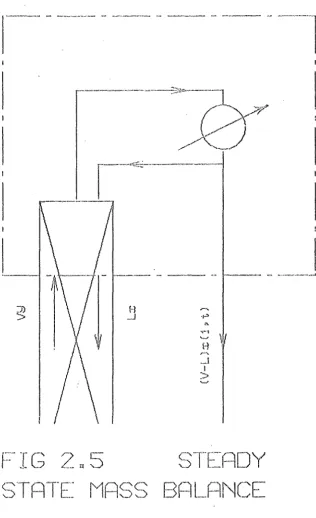
An explicit relationship between x and y ls Rlso given by a mass bAlance around the envelope shown in fig. 2.5, The moss balance qivcs:

V.y - L,x t (V·L),X(l,O) ••••• (2.20)

Any two of the three equations (2.1R) to (2,20) will qiv0 the solution for x(z) and y(z) at steady state. The choice of equations will depend on whether it is necessary to determine any of the parameters ( e • q • L, V, K a) to ~atch the boundary conditions. This choice will be

G

3.1 The Model rn Finite Difference Form.

3.1.1 The Oynandc 1·lass Balances, 3.1.2 Aounctary Conditions.

3.1.3 Initial Conditions.

3.2 Solution Of The Steady state Equations. 3. 2. 1

3. 2. 2 3. 2. 3

Reboiler Compositton Unknown. Subroutine FINDXB. R0flux Ratio Unknown. Subroutin~ FINDR.

Number Of Transfer Units Unknown. Subroutine

FINDTU.

3.2.4 Top Composition XD Unknown~ Subroutine FiNDXO. 3.3 · Sblution Of The Unsteady State.

z,

1 .. (J 1'·1 [J [J

r·1-1 rJ t:::J

M·-2

0

0

(J)

r·

0.

I~

1·1

a.

u

(/)

(JJ

I+1 [] (\$ _[]

·:)

(J)

1-

-+-:r

(.!)

1··1

ld

I

0

D

:r:

z:

5

..J

0 0

4 []

_Ll

3 D Cl

REBOILER

1

0

0

TI~·JE SUDSCFHPTS

F·-· ]" ['

r3

1

cornrosltlon variah.les and t <Jre in fig. 3.1. The first subscript indicates hclqht with represPntinq the H'boiler, 2 tt1e bottom of the ~'acldn<J, dnd m the top of the Pod:Jnq. '!'l)e second subscript shows the ntlJ",ber oE time interv<-lls :;incc an upset \'1<1S introduced into the column, Note that x is identical to XB, x to

xo,

m and that t ~ y

=

y •

1 1 2

x C and hence y

1 2

and x . TtJ.e problem is thus a srltt bound,Hy value fJi

problei11, since the boundary cond.ttions (Jive the Vdl\le of one v.-ni<thle at one end of the pack1nq and the other variable at the other end.

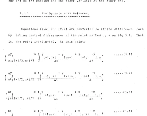
3' 1.1 The Dyn~rnic M~ss Balances.

Equations (2.6) and (2,7) are converted to finite ditferenc0 form

by taking central differences at the polrt mArked by ton fiq J.l. That is, the Point i+ll2,ni112. At this point:

a y

:;

1

v

-a

v

1-

y

··v

(

_a-z·

)

f

i + 1, n+ 1 i, n+ 1 .J.! ..

Lt~\-~--l..L!}...)

1 + 1 I 2 , n + 1/2

"?.\

---~z--··--- ₄₁ ,_

••• ,.(J,t)

aY

=

1 y - y + y -y

(''"aT)

it 1 I 2 'n + t I 2 -

;r( ~L~-~!!.!tr-

2

L~.!..!2~

"

J.L~~}.T

__ ,i_:.n .. )

•••.•• (3.2}

. , , , , ( ) . 3 )

oX ::: J X ~ X

( ) ( lH,nH Ht,n

· ---aT,

1 -• 1 12 , n + t 12

--,x

·1:\r---·-

---+

x

··x

__

L~!1_:

__

~

i\C_l

! _r:~.)

[image:31.600.40.535.398.787.2]

'!' h 0 :> c c C' n t: r e d d 1 t f e r e n c c a p p r o :< 1 rc <1 t i o r 1 ~; il rt' s e c o n cl o c d e r: c o r r i' c t •

The v

.n

u e s o t

v

i+l/2,n+tn

<1nd f drr~ taken as:

y

it1!2,n+112

f.

1+112,nt112

1tl/2,nf1/2

-- 0,25(y fY ty +y ,,,.,(3.!))

i+1,n+l i+1,n i,n+l t,n

- 0,25(f +f +f +f ••••• (3.6)

itl,n+l itl,n i,n+t i,n

These approximations are substituted into (2,6) and (2,7) to qlve:

AB,y

i-t 1, n ·f t

BR.x

i+l,n+l

where: i\J\

AH AC l\D AE: BA Bn

-- ~Afl,y + AF:(t + f + f + f.

1, n + l i+t,n+l t , n + 1 .i+l,n i,n

+ 1\C,y + i'ID.y ••••• (3,7)

1, n i+ 1, n

.. H3B,x

i,n+i

~ BA(y

.\+l,n+1

" f

+ y

i+t,n+t it 1 , n

J. !3C (X ~ ~<

J.,n .i+1,n+1

-

=b + c + 1 .•.

_\

_J_

/jZ '2 tH

-

+b + (." + 1

~-1 _1_

t:.z 2 ll.t

·-

+b n c ,~ ₁

1 ,__J_ l\ 7. 2 Llt

..

~b ~ c + ₁

,_.J

__ 1.

ll.Z 2 1.\t

-

c /2 1

--

c /2 2

=

··b ~ t

__ 1.

.6tJ

!JZ

t , n ·~ 1 .. f

f ,n+l

+ y

t,n

.t, n .

[1\.

-

+b

..

t

').

1\Z

'Ef.

\•: lH' n tF: 0 , til e t e r m < 1 I C. r. ) i ;, r <' rn o v e d f r o m tf) c d t.> t i n i t t o n !> f o r .~ 1\ ,

Afl, AC and AD.

(7.,9a).

3. 1 • 2

Also b

1

c1nd c dl'E' then clef.lnod by equations

1

Boundary Conditions,

(2,Ba) and

Taking central differences at time ntl/2 for the condenser equation (2.13) gives:

l!C(X - X ::: l),SV(y

rn,n+1 +

y

.. o.svcx

m,n+l

+ X . )

m,n rn,n

rn,ntl m!...!l....

~~·-

.c.t

which is rearranged to:

X ~ ( 1 .. C) X t C ( Y + Y ) , •• ,',(3.9)

m~n+l

m,n

m,n+l

m,n

( J +C) ( HC)

whore C- O.SCV.At/HC).

Similarly for the reboiler at time nfl/2, equation (2.15) is expressed as:

(HP/At)(X -X ,_ O.S(V'"L)(X t X )

1,n+1 l,n

m,n+l

m,n

+ O.SL(x + X • O.SV(f + f )

2,n+1 2,n l,n+i l,n

~~ h i c 11 y 1 e 1 d s :

l, n + 1

:::X + (O,Sflt/l!R)((Y-JJ)(X

l,n m,n+l

t X

X

m,n

t f, (X + X

2,nti 2,n

- v (

f + t )) ••••• ( 3 • 1 0)

3' J • l r. n l t .I i1 l C o 11 d i 1: 1 <) n s "

T lH~ in t U at con d i t 1 on e q \L1 t ions rn us t c1 l so b c (~ x press f.: d 1 n f in l t e difference form, so thJt they can he used ns the startinq point for a dynamic solution, T h e v a 1 u e o t x ?1 n cl y .t s n e c d e d <l t e c1 c t1 ctr t d p o 1 n t ll p the column. I.e. we need:

1, 0 y

i 10

as well ns the initiul reboiler composition x • l\s the initial conclit.ton

will usually be a steacly state condition, the steady state equations will now be written in terms of fi.nite differences. The tim~ subscript is dropped since x and y are time~independent at steady state.

Equation (2,20) in the new notation becomes:

y ~ R.x + Cl·R)X

1 1 m

Tak.ing centr3l differences we get:

iJY

(

~a?.)

i+ 1/2

::: y "' y

____li_L ___ _i /).Z

ax

=

x

.. x

( )

_DZ,

_1+1/2

_w __

fj.Z l~

y . .. 9.5(y i+112 / 1

£ •• 0.5(E

i H/2 .t

+-'l )

i +I

t f )

itl

Substitution in (2,18) anrl (2.19) 01ves:

Y (1/6z + 0.'5r! )

=

Y (1//.\Z ~ N ·~ 0,5N (t

1+1 OG 1

oc:

OG !tl

t f )

1

... (3,11)

X .. X ~ ( 0 , S !I • (').

z

I R ) ( f ·~ y ) . . . , , ( ) , ! 3 )

1+1 i llG i +t

The stendy state bounrlRry conditions in this notatlon ~re:

X

..

y •• ,.,(3.14)

m m

,1nd y

-

f . . . (1.l5)

2 1

3.2 SO!,UTiotl OF TfiE S'l'F~1\DY STATE EQUATIONS,

"

I. l

.,

/Is st<~ted tn section 2,•1.1, any tt•:o of enui3tlons (2,18),(2,19) and

(2,20) may be used to compute the values of x and y throtlghout the column at s t e ad y s t a t e • The c ll o l c e o t the c quat i 0 n s c:e Den d s on w he t ll € r any o f the variables XB, XD, R or N are unknown. Provided any three of these

fJG

four variables are specified, the fourth may be computed a~ong with the x and y composition profiles in the packing. fortran suhrout!nes were writtcJ\ to obtain the solutions in all four cases. The method is briefly outlined below and the subroutines are listed in appenrlix 2.

~/hen the steudy state composition proElles iHe reqllired, subroutine SSTATE is called, This subroutine will c~ll another dependlnq on which of the four variables is unknown.

3. 2 ., 1 P e h o i 1 e r C o r:1 p o s 1 t 1 on ll n k n o w n •

s

ll h r o u t i n e I' lliD X B •

This subroutine is uscct when R,N and XD are known. Startln~l

OG

from the known top composition, it evaluates x and y moving down the

co lu rn n 11 s 1 n C! e ou u t 1 on s ( 3 • l t ) d n d C3 • 1 2) • The e q u ll i b r i urn r e 1 a t1 on s h .l p sunroutlne, YST/\H1 1s tl1en used iterativelv to tinrl the value of XB which hrlS an equilibrium V·1lue f

1

equal to the corr,ptJted V<llue ot y •

3.2.2 R 0 r· lux Fat i o ll n ~~no·.~ n • · sub rout 1 n e f.' HID 1< ,

Tl1.is subroutine is used whr.n XEI, XD und N are ~recified. The OG

value of R is set first to \.0 and adjusted until the value of XH calculated by fiNOXB is e~ual to the specified value of XB, The initial step !.n

n

is (1~n )/2 and the step size .ts halved at eacl1 step, R

min ml.n

is the minimum reflUX ratio whlch will qjve the required separation,

3. 2. 3 Ntl!nber Of Transfer Units Unknown. Subroutine FINDTLI.

With XO, XD and R specified, the numher of transfer units is computed numericallY uslnq the equation :

N ::: ••••• (3.15)

OG

subroutine FINDXB is then used to find the composition profiles in the column.

3.2.4 'l'op Composi.tion XD llnl<nown. Subrout.ine F'TNDXD.

B e c a u s e e q u a ti o n ( 3 • 1 1 ) r e q u i r e s p r i o r l< no 1v1 e d q e o f: t l\ e v a lu e o t

XD (i.e. x ), it is better to use equations (3~12) and (3.13),

m

These

s t i 11 need an in .tt .1 a 1 g u e ~' s of the v a 1 u e o f f at e a c !1 p o 1 n t 1 n the column. Subroutine FINDXD does this by assuming at first that f varie~

linearly __ w1tl1 z, . and then t.tpdates the f _ yalu0s_.c~t each succ:eedinq __ iteration until converqence is obtained.

The first attempt at writing FINDXD made use of equations (3.11) and (3.12), A value of XD Was assumed for use in eauation (3.1 1) and was then compared with the value of x found by 1nteqratin0 up the column

m

[image:37.603.197.555.25.787.2]

for hlqh r~flux r~tlns, but for low r0tlux rdtios (s0y 11_<0.81 1

column was then l.n a vc~ry tlql)t Pinel) zor1e, <lnd <3 sw,~lt error ln the

d s s u m c d v a 1 u e o t X D c i) u s t~ d <l v e r y .1. i:l r q e e r r o r i n U1 c v <:11 u e o f X D o b t a .l n c d by integratinq up the column.

3.3 SCJ!,tlTION CW Tl!r~ lH!STE;i\DY ST,\'l'E,

I t i s r e q u .i r e d t o co !11 p u t e x , y and E a t t i me n + 1 'll hen a ll v i.l 1 u e s at time n are known. (When n=O, then x and y are given by the initial ste<ldy st.:1te).

Since y is given from the reboller boundary condition, 2,n+1

equ~tion (3,7) would enable y to be found explicitly ~or i

=

3,4 ••• m if .'3J.l the f.··

.l,n+l

i,n+t

were known. As they are not, an iterative solution is

required. ~or the first iteration at time ntl, it is assumed th~t

£ ·~ t For subsequent iterations, the values of f are

.i,n+l i,n J.,nt1

undated after the x have bePn found. After all the y values at time i,n+l

n t 1 t1 ave been e s t i rna ted f r om C .'3. 7 ) , the conde n s e r b o u n cl a r y con d .l t 1 on i s used to qivo x Equation (3.8) is then used to compute the x values

ro, n+ 1

working down the column. from the values of x thus obtained, the values of f at time n+l are then updated, After the reboiler_boundary c9ndition has been used to update the value of y , a further iteration can be

2,n+1

m a de a t tt1 e s a rn e t i rn e • I t v: A s t o u n d t h a t t w o i t e r a t 1 o n s <t t e a c h t i m e step usuallY gave a converqcnce 111 all the cornrositions to within 0.0001

mole fraction. The decision to proceed to the next time st0p may be

based on so1ne converqr:nce crlt0ria, or a fl:.:ed ntlrnter of lteratlons at

in tlq. 3.2.

It L, V, H or K a are exrected to vary with composition, time, or G

~osition in the column, the coefficients in equations (3.7) and (3,8) can be updated at eacl1 time step. They would then be vectors, rather than constants, with a value for each height interval in the column.

A fortran rroqram to calculate the transient solution is listed In appendiX 3. I t .is called I,IAINLINf·:t.

3,4 TRUNCATION ERROR IN TH~ UNSTEADY STATE SOLUTION.

von Rosenberg(1969) shows that for a single dependent-variahle, hyperbolic, partial differential equation, there is zero truncation error in the .finite difference approxim~tion provided tl1at 6z/At

=

b. With two dependent variables, a choice must be made between usinq b and b to set

1 2

the time interval. It was decided that Az/At - b should be used. lt 2

seems reasonable to try to minimise the truncation error in the ~iquid

composition, because the liquid holdup has a much greAter bearinq on the column dynamics than does the vapour holdup. On comparing the results of solutions with different sized increments, it was found that there was no truncation error for Az/At

=

b provided that Az was not greater than

2

TABl,E 4~ l OPERATING CONDITIO!.JS f:JSI RUNS 0ISCUSSI~D l(J Ci-iAPTER 4 ..

Variable Run 1 2 3 4 5 6 7 8 9 10

Ir;itial XP.

0.2000 0.2000 0 .. 1052 0"1052 0~1052 0.1052 0~1052 Ow0500 Oc05()0 002000

Initial XD Oe6787 0~6825 0.8560 0~8000 0.7648 0 .. 6337 0.5408 0 .. 98)_1 Oo4566 Ge6825

Final XD

O.a6525 OV<5432 0,.7247 0.7247 0~7247 0.7247 0~7247 0~4566 0~9811 0~6315

I:titicl R 0@82 0 .. :3 () 1'"'00 0 .. 90 Oo85 0.70 0 .. 60 1.00 n _{\.)"" )} C''"l _{J':- Oil80}

F.inal R 0 .. 80 0~70 0080 OQ80 0 .. 80 0.80 0980 0992 1e.OO 0.70

IJTU 4c0 5~0 8~0 8~0 8QO 8.0 8.,G J 0 i 0 10~0 5 ~ r;

Time interval L25 1 e 4 3 J.o25 L25 L25 1. 25 1.25 L09 L00 11¥43

T~e following variables were the same fer most or all runs:

vapour holduo

=

o.o

liquid holdup

=

10.0 condenser holduc

=

0.0 reboiler holdup

=

infinity

C=

50.0 for run 10) packing height

=

10.0 height i~terval

=

0.1

3 1

CliAPTEH 1\ nr·:SUWS (Jl" THr~ CO\IPUTEH SnLtJTION Ol,' THf·: r.HJDEL,

4.1 Typical Results,

4 .1.1 F:xilmples Of Ne<H"L.tnP.ar F'irst. Order Pespon:>c Curves, 4.1.2 Examples Of Non~Linear Response Curves,

4.1.3 Cornpar.tson. ',Hth Results Of Tonwssl. lind Hice, 4.2 Pitting Of 'Time Constants' To The Transient

Responses.

4, 3 Effect Of Colun'n Ho tdups,

The model was ust:d to compute the response of the basic column to step changes in reflux riltio for a wide range of operatir1g conditions. The responses were all computed assuming that the height of a transfer u n 1 t , h o 1 d u

r

s a n d v a p o 11 r r a t e d i d no t v a r

y

w t t h p o s 1 t 1 on o r t .t rn e ,

so

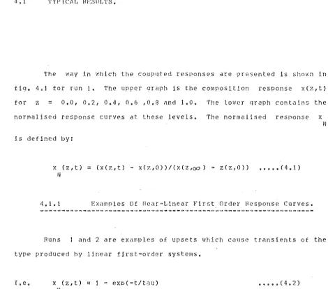
f11 e results are illustrated and discussed in this chapter, The operating conditions for the runs considered are listed in table 4.1.

'f' he w 2t y in w 11 i c h the co n1 put e d r e s p on s e s a r e p r e '5 en ted 1 s s hoi'.' n in

tig. 4.l for run 1. The upper graph is the cornposltion response x(z,t) for z -

o.o,

0,21 0.4, 0.6 ,0,8 Rnd 1.0. The lower qraph contains the normalised response curves at these levels. The normalised resronse x

N

is defined by:

X ( Z 1 t ) ::: (X ( Z. 1 t ) - X ( 7, 1 0 ) ) / (X ( 'l. tOO ) • Z ( Z 1 0 ) ) • • • • • ( 4 • 1 )

N

4. 1. 1 Examples Of Hear-Linear First. Order Response Curves.

Runs 1 and 2 are examples of upsets which ca11se transients of the type produced by linear first-order systems.

I.e. x Cz,t) - 1 - exp(-t/tau) N

••••• (4.2)

or: x(z,t) = xCz,O) + CX(Z1<:1-') - x<z,O)).(l- exp(--tltau))

For run 1 (ffq. 4.11 1 the composition chanqes were very small and

[image:43.598.52.522.77.491.2]

The equilibrium curve for runs 1 and 2 was based on the data nf

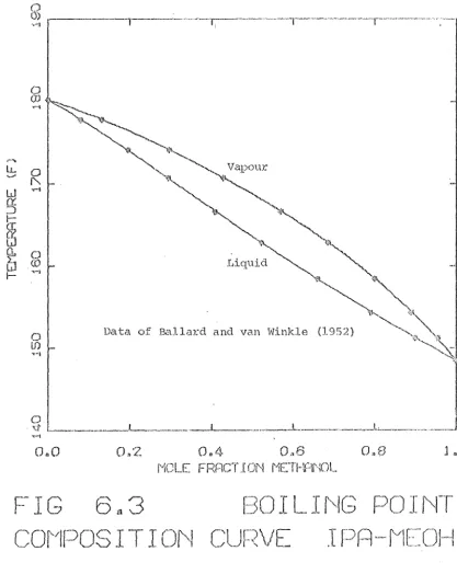
B,11l·1rd And ve:m \Hnkle ( 1952) for isopropanol and methanol. For runs 3

to 7 a linear equllibrjum relationship:

f. -- 0.2 t O,B X

was used. Vor these runs1 responses fitting equation 4.2 were obtalned,

even tor large chanqes in reflux ratio. However for large upsets, the 'time constants' tenrled to depend on t11e position in tl1e column. For runs 3 to 7, the transients were computed for varying initial reflux ratios with the same final reflux ratio of 0.8 in each case.

shows the response tor run 3 and fiq. 4.4 shows that for run 6. The rlependence o.f the 'time constant' on column position was obviously greater tor the larqer change (run 3) thnn for the smaller one (run 6), The response at z=l

.o

for runs 3 to 7 is plotted in tig. 4.~. I t shows

the 'time constant' to be almost independent of the initial steady state, varying Erom 18 time intervals for t'lln 3 to 15 time intervals for run '/, However at z=O.O, the 'time constont' varied froin 11 to 23 Ltme intervals for the same runs •

. ·

.

4 .1. 2 Examples Of Non-Linear Resronse Curves.

·"---~---In this section, some results are shown where eq11ation 4.2 would have to be extended to:

x (z,t)

=

N

n

·~

\.-,, c ex p (

~tIt

au )

L

1 1

i=l

••••• ( 4 • .3)

to adequately descrihe the composition response curves, rn equation 4,3

=

1.0 and the number of exponential terms, n, 'HO\Jld usually

from 1 to .1.

a t t l1 e b e \li n n J n g h u t u f l e r s o m e ti me h a d e 1 a p s e d , s how I n q t h u t: a l i n e a r t1rst--order response did not clescribe It, In run 9, the rr~f:.lux ratto wa~;

the reverse of that in run B. The response was now most rapid at z=I.O and slowest at

z:o.o.

The reasons tor this chaJ\Qe in response time with position in the column i:lnd direction of reflux ratio chccmge can be explained in terms of the composition drivlnq force f-y. Recalling equation 2.4:

Hax

=

Lax - K a.sct-y)

G

at

zaz

••••• (2.4)

it can be seen that the rate of change of compo3ition

ax/at

at a given height is proportional to the difference between (L/Z)Cax/at) and K a(f•

G

y) at that level. At steady .state, these terms are equal. Obviously .it part of the column is in a pinch zone, where the operating and equilibrium lines are very close, then both terms on the right hand side of equation ~.4 must be small. Therefore the rate of composition change

ax/at

must also be small, since it depends on the difference between two

small terms. If (f-y) is larqe, then ax1az will also be large, so that when a change is made in the liquid rate, the difference between the two terms on the right hand side of the equntion may also be large. This means that if the driving force is larqe for any level in the column at the start of a transient, but small at the end of it (e.g. z~~o.o in run 8), then the composition response at that level will initially be fast, but will slow as the transient proceeds. Conversely if the composition driving force is small at the start of a transient, but large at the end (e.g. z~t.o for run 8) 1 then the response will be slow at fJrst, but Will speed up as t-y increases, and will eventually slow down as the new steady state is rea~hed. This arqument may be generalised as follows: the normalised composition response to a step change in reflux ratio will initiallY be fast nt those levels which are moving Lnto a pinch zone, and slow at those levels which are moving out of a pinch zone.

35 the response is slowest from the reflux rdtlo of 1.0 and fastest trom that of 0.91, This is because for R

=

1.0, XO

=

0,98\ and the column must move out of a tiqht pinch zone at the top. For the inltlal reflux ratio of 0,94, XD

=

0.5R8 and the response WclS raplrl In this case because the top of the column was not in a pinch zone.

The shape of the response curves has been shown to depend on the initial and final steady states as well as on the position in the column. Because of the large number of variables involved, there seems to be

little point in trying to relate the coefficients and 'time constants' of an equation such as 4.3 to the parameters of the column being studied. Instead, if the composition at any level is required at a particular time, or as a function of time, this can be simply computed by the model as it stands. The comput~r solution is at least 100 times faster than the real time scale, so the mo~el is suited to on-line work provided that the computer has sufficient storaqe. The time taken for the computer solutions, and the storaqe requlrements₁ are dlscussed 1n appendiX 3,

Comparison With Results Of Tomassi And Rice.

The results of Tomassi and RlceC1970) are used as an example of the results of a model. using a linear equilibrium relationship, in order to make a comparison with this study. Tomassi and Rice used an equilibrium curve linearlsed so that the computed compositions at the ends of the column at initial and final steady state matched their experimental values. This required prior knowledge of the final steady state. Their computed transients had the form:

n

xcz,cO) " x(z,t)

~

2}

_i i=l

exp(s t ) i

••••• (4.4)

This is similiJr to equation 4.3 GXcept that jn 4.4:

'c

=

xcz,OO) ~ xcz,t)

L' i. and

s ... -1/(t.au ).

i i

36 so t h <> t \--c ::: 1 , w o u l d <l e pend on l y on z and the f: in a1 s t 0 u d y ::; tate :

L i

w l1 i 1 e the f 1 r s t t 5 1n e cons t. d n t :> J s e 1 t her J. n dePendent of , or a s 1 ow 1 y

v a r y i n g f u n c ti o n o f , z • D n UH· b a s i s o £ tiH e (' r u n s £ r o rn d 1 U e r e n t

initial reflux ratios to the s~me final one, Tomassi and Rice concluded that the time constants depend on tl\e final stf'Cidy ;,tate, but not: the magnitude of the cl.l.sturtHllK~~ or the inltlal steady state, \~e h·'lVe already seen in section 4,1 .1 that this need not be true. In runs 3 to 7 where the final steady state was the same in each case, the 'time constants' varied from 18 to 15 time intervals at z

=

t.o,

and from 11 to

23 time intervals at

z

=

o.o.

Tomassi and Rice state that linear theory predicts that the 'time constants' should be independent of z. They obtained this result when

R

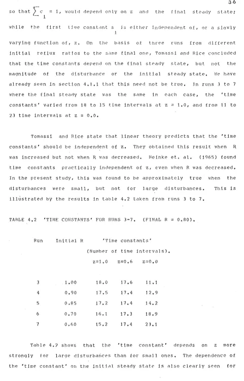
was increased but not when R was decreased, Heinke et, al. ( 1965) found time constants practically independent of z, even when R was decreased. In the present study, this was found to be approximately true when the tlisturbances were small, but not for large disturbanc(~s. Tl1ts is

ill~strated by the results in table 4.2 taken from runs 3 to 7.

TARl,E 4.2 'THlE COHSTJI.NTS' F'OR HUNS 3-7. (FH!i\I, R- 0.80).

Run Initial R • T i me con s t a n t :; '

(Number of time jntervalsl. z.::::l.O z=0.6

z:::o.o

3 1.00 Ul.O 17. 6 11 • 1

4 0,90 17.5 17.4 12.9

5 0.85 17.2 17.4 14.2

6 0,70 1 f) • 1 _17.3 18.9

7 0,60 15.2 17.4 2 3. 1

[image:50.597.56.538.51.804.2]

37

z:::o.o.

Both Heinke et, al. and Tomassi ar.cl Rice tOJind, as the latter authors put it, "the relaxation time usually increased from top to hottorn in experiments in which the reflux ratio was changed from a lower value to a hlglier value, and decreased when the reflux r<Jtto was chanqcd from a higher value to a lower one". These observations are explained by the column being in a pinch zone at the tor for hiqh reflux ratios but not tor low reflux ratios.

4.2 FITTING OF 'TIME CONSTANTS' TO TH~ TRANSI~NT RESPONSES.

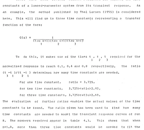
There have been several schemes published for tinding the time constants of a lumped-parameter system from its transient response. As an exantPle, the method published by Tl1al r~arsen (19~15) is cons.idered here. This will find up to three time constants representing a transfer function of the form:

G(s)

=

( t.Ju s·~ 1) c tau s tT)muStiT

1 2 3

To do thls, it makes use of the times t , t , t requ1re0 for the

1 2 3

normalised response to reach 0.1, 0,4 and 0,8 respectively. The rotio

( t ·t )/(t -t ) determines how many time constants are needed.

3 2 1

For one time constant, r u t 1 o ::-: 3 • '12 5 ,

for two time constants, 3.725>ratio>2.92, for three time constants, 3.725>rat1o>2,68,

[image:51.600.67.538.370.793.2]

38 response, but at z=O,O anrl z=O.~ the response Js initially too rapid to

be represented by even a single time constant.

TARLE 4,3 NUMB~R OF 'TIM~ CONSTANTS' FOR TRANSIENTS OF RUN 8.

z t

1 t

2

t Ratio Number of time constants

3

1.0 31 77 133 2.20 >3

O.R 1 8 56 107 2.34 >3

0.6 8 32 77 2.88 3

0.4 4 1B 53 3,63 2

0,2 2 11 40 4.22 <1

o.o

1 8 33 4.57 <1

These results reinforce the conclusion drawn in section 4.1.2: that there is little point in trying to represent the non-linear distributed-parameter system as a linear lumped-parameter system, especially since the response of the distributed-parameter system can be obtained rapidly usinq a digital computer,

4. 3 EffECT OF COLUI-1N HO!,DUPS,

For the runs described in section 4.1, the column was assumed to have zero vapour holdup, zero condenser holdup, and infinite reboiler holdup. Further runs were done to find the effect of including these holdups. Run 2 (fig. 4.2) was used as the basis for comparison. The total holdup in the packing for run 2 was 100 moles.

( f ) Effect of vapour holdup. Runs were done tor h ranqinq from 0.1 to

Table 4.1 qjves the 80% response time (J.e, the time at Which the normalised n~sponse reaches 0,8) tor ditterent rlt~iqhts in the rackinq tor various vapour holdups. lt sl1ows that the efff'ct of the vapour holdup on the response time is small until the vapour holdup exceeds 10% of the liquid holdup, This is unlikely to happen in columns operatlnq at atmospheric Pressure.

TARLE 4.4 EFFECT OF VAPOUR HOLDUP ON RESPONSE TIME.

z

h ::;

o.o

0. 1

o.o

17 17

0,6 1.9 19

1.0 19.5 19. 5·

0 o:l ,.

17 19.5 20

1.0

18

20 21

2.0

1 9 21

22.5

5.0

21

25 27

0 00 00 -·--····-T-·

---+LJ:i

___

·y--·-··-~···--~· ... 0 ' ... co

.

0 00 00 .-1 \1) 0 U" I, E

m

(()

.

0

"''

' 0 N

.

0 NO LU SOct--:08 0 TriO rl 0 rl II N co "' 0 0 II :1 N t~ 0 0 a N ___ _t ____ -~L 0 co (!) ~

.

.

' ' ~· 0 0 0 () Nor usoc'WJ8 ornon · o·o ' ., Orl ()j

•

0 gj '.0 ' 0 o;;t ' 0 N ' 0 0

.

0 3SNOc3J~ NOfliSOd~08 OJSfl~cON 00 (J) (0 ·J N 0 '

.

.

.

.

() ,.., 0 0 0 0 0 0 (l) 0 '<:]' (f) .J o·

>

(I (J t;: L. >-t lo) L: :0.-t 1-l• 0

ei

}~

L: (f) _J ~

rs

tz:

H ~~

,_,

~-t5

~

0