Linear Maximum Likelihood Regression Analysis for Untransformed Log Normally Distributed Data

Linear Maximum Likelihood Regression Analysis for

Untransformed Log-Normally Distributed Data

Sara M. Gustavsson, Sandra Johannesson, Gerd Sallsten, Eva M. Andersson Department of Occupational and Environmental Medicine, Sahlgrenska University Hospital,

Academy at University of Gothenburg, Gothenburg, Sweden Email: [email protected]

Received June 25,2012; revised July 27, 2012; accepted August 10, 2012

ABSTRACT

Medical research data are often skewed and heteroscedastic. It has therefore become practice to log-transform data in regression analysis, in order to stabilize the variance. Regression analysis on log-transformed data estimates the relative effect, whereas it is often the absolute effect of a predictor that is of interest. We propose a maximum likelihood (ML)-based approach to estimate a linear regression model on log-normal, heteroscedastic data. The new method was evaluated with a large simulation study. Log-normal observations were generated according to the simulation models and parameters were estimated using the new ML method, ordinary least-squares regression (LS) and weighed least-squares regression (WLS). All three methods produced unbiased estimates of parameters and expected response, and ML and WLS yielded smaller standard errors than LS. The approximate normality of the Wald statistic, used for tests of the ML estimates, in most situations produced correct type I error risk. Only ML and WLS produced correct confidence intervals for the estimated expected value. ML had the highest power for tests regarding β1.

Keywords: Heteroscedasticity; Maximum Likelihood Estimation; Linear Regression Model; Log-Normal Distribution; Weighed Least-Squares Regression

1. Introduction

Measurements in occupational and environmental re- search, e.g. exposure and biomarkers, often have a skewed distribution with a median smaller than the mean and only positive values. It is also common with hetero-sce- dasticity where the variance increases with the expected value. Such data can often be described by a log-normal or quasi-log-normal distribution [1].

Associations (for example between exposure and health effects/biomarkers or between personal exposure and background variables) are often analyzed using re- gression models. Ordinary least squares (LS) regression analysis is a commonly used regression method, and it is based on the assumption of a constant variance and a normal distribution for the stochastic term. One way of handling non-normal data is with nonparametric median regression (or Least-Absolute-Value regression), see e.g. [2] where no assumptions are made about the distribution of the response variable. The parameter estimates are then found by minimizing the sum of absolute value of the residuals (whereas LS minimizes the sum of squared residuals). However, as a nonparametric method it re- quires larger samples and it may have multiple solutions [3].

In situations where the response variable has a skewed distribution and an increasing variance, it has become the practice to log-transform the response variable. Regres- sion analysis on log-transformed data have for instance been used to establish reference models [4], to find suit- able biomarkers [5], to determine suitable surrogates for exposure [6,7], and to estimate the cost function in health economics [8]. A model in which the response variable is log-transformed, ln(Y), will estimate the relative effect of each predictor, whereas in many cases it is the absolute effect that is desired [9]. It must also be considered that e.g. a t-test for comparing the expected values of two groups based on the mean of ln(Y) is not equal to a test based on the mean of the original log-normal data Y, since the expected value of Y is a function of both μ and σ, whereas the expected value of ln(Y) is a function of only μ. If the two σ-parameters are not equal, a t-test based on ln(Y) may not give the correct type I-error re- garding the difference between E[Y1] and E[Y2], [10,11].

In many cases a linear relationship between the re- sponse and the predictor (e.g. between personal exposure and background variables) is a reasonable assumption; for example it is realistic that the personal exposure in- creases linearly with time spent in a certain environment (e.g. time spent in traffic). This linearity will be lost in a

log-transformation. On the other hand, if the log-normal distribution is ignored in order to preserve the linearity, tests based on the assumption of a constant variance may give misleading results, [12].

There is a need for methods that handle log-normally distributed data in linear regression models, based on moderate sample sizes. In order to estimate the linear association (and the absolute effect), but still take into account the log-normal distribution with a non-constant variance, we propose a maximum likelihood (ML) based method for regression analysis. In this paper we have evaluated this new method using large scale simulations, which allowed us to analyze the bias, variance and dis- tribution of the regression coefficients resulting from the new method, as well as comparing it to LS- and weighted- least-squares (WLS) regression analysis. A data set on personal exposure to 1,3-butadiene in five Swedish cities was used to illustrate the three methods.

2. Data

We considered the situation where the response variable

Y is assumed to follow a log-normal distribution (i.e. ln(Y) is normally distributed) and where the expected value is assumed to be a linear function of the predictors,

 

0 1

E Y X 1

Y Xp p.

       



In regression analy- sis, some X-variables can be included because of known (or suspected) association with Y, in order to decrease the variance or lower the risk of confounder effects [5]. Since Y follows a log-normal distribution, ln(Y) can be expressed using the following model

 



2 _{2 ,}

p Z i

X   e



2

e N

0 1 1

ln Yi ln  X    p

where i~



0,Z . The k

model above. Linear regression analysis on the log- transformed data would yield an estimate of the relative effect of Xk, rather than the absolute effect. This is illus-

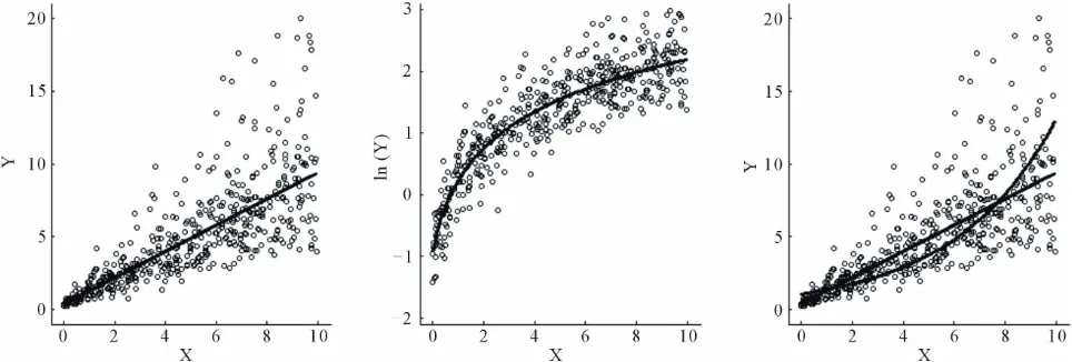
trated in Figure 1.

A log-transformation is not suitable in situations when the aim is to estimate the absolute effect of X on Y (rather than the relative one). In a licentiate thesis [13] it was suggested that the linear regression should be estimated from untransformed log-normal data using maximum likelihood methods. In this article, the properties of these maximum likelihood estimates will be evaluated.

2.1. Simulation Study

The properties of a new method for statistical analysis can be derived theoretically and/or by simulations and examples. In a simulation study, a model for the variable of interest (here personal exposure) is used to generate samples of observations, 1 n and then the pa-

rameters under investigation (here regression parameters) are estimated from each sample. This is repeated to ob- tain a distinctive distribution for the estimates. Our simulation study allowed us to assess the bias and stan- dard errors of the parameters estimated resulting from the new maximum likelihood-based regression analysis, and compare these results to those of LS and WLS.

, ,

y  y

We used simulation models in which the response, personal exposure to Particulate Matter smaller than 2.5

μm (PM2.5), was assumed to be a linear function of back- ground variables (residential outdoor level of PM2.5, smoking and time spent in home). Two different simula- tion models were used to generate data. Model A had only one predictor, the personal exposure to PM2.5-parti- cles (μg/m3_{), Y, was assumed to be a linear function of} the residential outdoor concentration of PM2.5 (μg/m3),

ConcOut. Model B had three predictors and no intercept, ˆ

 is an estimate of the absolute effect of Xk on Y. The log-transformation results

[image:2.595.57.539.530.693.2]

in a distortion of the linearity, as can be seen in the

Figure 1. A linear regression where Y|X follows a log-normal distribution. The absolute effect is 0.9 (left), the log- transformation stabilizes the variance but distort the linear relation (middle) and the estimation based on log(Y) result in an

xponential function with a relative effect of 29% (right). e

Y was a linear function of the number of cigarettes per day, Smoke, number of hours spent in their own home,

Home, and residential outdoor concentration of PM2.5 (μg/m3_{), ConcOut. Since ConcOut > 0, its regression} coefficient can be interpreted as a stochastic intercept. Datasets were simulated by generating normally distrib- uted observations from Model A:

 





_{0.354 2}2 _,

i  ei



_{, }2 _0.3542







ln Y ln 4.803 0.574 ConcOut

where i Z . Samples from Model B

were simulated according to

~ 0

e N

 

2 ln

ln 2.092 0.761 0.450 2 ,

i

i Y

Smoke ConcOut

e

   

 

0.218 Home

 



_, 2_{0.450 .}2



where _{i Z} The parameters in the simulation models,



_{0 1}



~ 0

e N 

, , _Z

   and



   ₁, ₂, ,_{3 Z}



ˆ

E

, were estimated from real measurement data (Johannes- son et al. [14]).

The number of repetitions needed in the simulation study was estimated. In order to obtain a 95% confidence interval for  

  that is smaller than 2·0.0005, 4 mil-

lion samples were needed. For the predictors, discrete values were used: ConcOut = {2, 8, 14}, Smoke = {0, 7, 14} and Home = {8, 16, 24}. Sample sizes n = 108 and n

= 216 were used in the simulations and the data sets were balanced with regard to the predictors. For Model A a second set is also created with a data structure similar to the observed one in the original dataset [14], which was slightly unbalanced.

2.2. Application to Exposure Data

The properties of the three regression methods (LS, WLS and ML) were illustrated using a set of data on personal exposure of 1,3-butadiene from five Swedish cities. 1,3- butadiene is an alkene and has been listed as a known carcinogen by the International Agency for Research on Cancer (IARC). Traffic and exposure to tobacco smoke are considered to be two sources for personal exposure to 1,3-butadiene [15,16]. Wood burning has also been showed to increase personal exposure [17]. The dataset was collected in a study of exposure to carcinogens in urban air in five Swedish cities; Gothenburg, Umea, Malmo, Stockholm and Lindesberg, see [18], and con- sisted of 268 measurements of personal 1,3-butadiene exposures. Background data were collected by a ques- tionnaire.

3. Methods

In our investigation, the outcome variable Y was as- sumed to be log-normal with an expected value that was a linear function of the predictors;

1, , p 0 1,i 1 1,p p

Y X X x x

 _      

From the simulated data, the parameters of the regres- sion model were estimated using ordinary least-squares and weighted-least-squares estimation as well as maxi- mum-likelihood estimation, as described below.

3.1. Least-Squares Estimates

As mentioned before, the inference in ordinary least- squares regression method, LS, is made under the as- sumption that _{Y X ~ iid ,N}



_{ }2



2 2 i Yi Y i,

,

Y i Y

where

 

2

ˆ MSE

 

ˆ

. The standard deviation is assumed constant for all Y and Y . The covariance matrix for the vector LS is estimated as

 

LS





1 ˆ

cov  MSE X X 

ˆ

, where X is a n × (p + 1) matrix. The standard errors,

SE(LS), are estimated from the diagonal elements of

 

ˆ cov LS .

3.2. Weighted-Least-Squares Estimation

For data that cannot be considered homoscedastic, there are several estimation procedures, for instance the White heteroscedasticity consistent estimator (see e.g. [19], p. 199). Since Y is assumed to follow a log-normal distri- bution, the nature of the heteroscedasticity is known;



2



2 _eZ ₁ 2

, i

Y i Y

   

2

. The variance is a function of the expected value. Thus weighted-least-squares regression analysis, WLS, is appropriate, in which each observation is weighted using W_i_Y_i

2 2

, ˆ

i i LS Y

W Y

. The weights can be esti- mated from the LS regression; _  __i

WLS ˆ



. The co- variance matrix for the vector is estimated as

 





1

WLS ˆ

cov MSEW



 X'WX



, ,

y  y

0, , ,1 , .

3.3. Maximum Likelihood Estimation in Regression

The maximum likelihood estimator (MLE) of some pa-rameter θ is the value at which the likelihood function

L(θ) attains its maximum as a function of θ, with the sample 1 n held fixed. The log likelihood is often

more convenient to work with and since the logarithm transformation is monotone, the function log L(θ|y) can be maximized instead. For a continuous variable the like- lihood function is the same as the probability density function, pdf. The MLE of θ can be found by differenti- ating log L(θ|y) with respect to θ. When θ is a scalar it is enough that the likelihood function is differentiable to get a direct estimate of θ. In a regression analysis, the aim is to estimate the parameter vector

p Z

  

  

   

θ

1, 2, , n

y y  y

.

Let be a log-normal sample where

ˆ

i

 

i 0 xi 1

E Y   



2



~ _i,

i z Z

Y N

.

Then ln

 

 





where 2

0 1 σ 2

zi ln xi  Z

   

and the log likelihood function is

 

 









2

2 ln .

Z i

i y

 



2



0 1

2

ln ln ln 2π

2 1 ln ln 2 Z i i i Z n L n y x            

The derivatives were previously calculated by Yurgens [13] and are given below with some corrections:

 

2 ,

2 Z

i ij j

j          _    2

ln 1 ik _{ln ln}

i

k Z j ij j

x

L _{y x}

x       _  



 _







 

2 2 2 ln 1 1 ln 2

n y ,

2 Z i   _         _{ }   l m k ik im ij j i j

Z _{j ij j}

L x x x x     _          _{ }   





 

2 , 4 3 Z

ln 1 _{ln ln} Z

i i

i j

Z Z

L n _{y x}

j j n            _    



_{ }



_    

 

2 3 ln 2 ln ln ik i l

Z k Z j ij j

x L x       _{  } 

 



 _ yi xill ,

      





 

2 . 4

i ij j

n

y x 

      _   , , , , 2

2 2 4

ln 3 _{ln ln}

i j

Z Z Z

L n

  

 _{  }







_



The maximum likelihood estimates of

0 1 p Z

   

 

  

0 1 ˆ ˆ_{, , , ˆ}



θ can be found by iterations, for example the Newton-Raphson algorithm, see [20]. The covariance matrix for the vector ˆ   Z

ˆ i



θ is

estimated by the inverse of the observed Fisher informa- tion matrix (see e.g, [21]), where the elements are the negative second derivative of the log-likelihood. One of the known properties of MLE is, under some regularity conditions, its asymptotic normality; when the sample size increases the MLE of θ tend to a normal distribution with expected value θ and a covariance matrix equal to the inverse of the Fisher information matrix (see e.g, [21]).

3.4. Descriptive Statistics and Inference

In the simulation study, samples of log-normal observa- tions were generated and three different methods were used to estimate the regression coefficients. The results from the three methods were compared using expected value (mean), standard error, bias, skewness, the 95% central range and correlation of the regression estimates.

The standard error of  was denoted SE _{ }

ˆ i

and

 

ˆ

i se

the sample specific standard error for  ,  , was the estimate of SE _{ }ˆ_i . The bias of an estimator,

i i

ˆ

E  _{ }  , was used as a measure of the systematic error. The skewness of an estimator was estimated as









3

ˆ ˆ ˆ

E E SE

  _   _{ }  _{ } _. For log-normal data, the

 



2



2

e 2 e 1



skewness is    , while a symmetric distribution has γ = 0. It has been suggested that a sample with skewness less than 0.5 should be considered as ap- proximately symmetric while skewness above 1 may be considered highly skewed. The 95% centralrange, CR95, was defined as the difference between the 2.5th and 97.5th percentiles. The sample-specific standard error of

ˆ_{Y X}

μ is

 

₂

 

2





1

ˆ ˆ ˆ

ˆY X p i i i j cov i, j ,

i i j

se μ x se  x x  

 





 







ˆ ˆ_,



i j

cov where x0 = 1 and  

ˆ ˆ cov _i, _j

is the sample specific estimation of  







* _0, .  

The inference properties of the three methods were evaluated by comparing the results from tests of the null hypothesis H0:β = β*, where   T in which βT is

the value specified in the simulation model. LS and WLS estimates was tested with the t-test,

  

ˆ ˆ

  

ˆ

t      se  , which follows a Student’s t-dis- tribution. The ML estimates were tested using a Wald- type of test statistic, which utilized the large sample normality of the ML-estimator and the observed Fisher information. Under H0, the Wald statistic

  

ˆ ˆ

  

ˆ

W  _  _  se 

tribution and

asymptotically follows a N(0, 1) dis W

 

ˆ 2 asymptotically follows a chi-

, see e.

n used on

4. Results

e presented in four sections; the distribution square distribution g. [21], Section 9.4. Other pos- sible large-sample test procedures for ML estimates (not used in this study) are the score statistic and the full like- lihood ratio statistic, see e.g. [21]. We chose the Wald statistic because of its computational advantages.

The properties of the test statistics above, whe log-normal data, were evaluated by the risk of type I error and the power. The true probability of a type I error for a specified nominal α-value (denoted α*_{) was esti-} mated as the proportion of test statistic values beyond the respective critical value. The power results were based on simulations in which the tested parameter (e.g. β0) was varied according to H1 whereas the other parameter (e.g. β1) was held constant.

Copyright Res. OJS of ˆi and ˆZ , predictions



ˆY X



, inference and an

app ation to xposure data folic e r 1,3-butadiene.

4.1. The Distribution of the Estimates

all three

ˆ

SE

1. Of the three methods, ML gave the smallest   i ,

11% smaller than that of LS. For LS, se

 

ˆ0 overesti- mated SE  ˆ0 by over 35% for the balanced data and about 18% for the unbalanced. For all three methods the standard error increased when unbalanced data were used. LS had the largest CR95, while ML has the smallest (the differences were around 12% between LS and ML and For data generated according to Model A,

[image:5.595.64.538.212.710.2]

methods produced unbiased estimates of the β-coeffi- cients (the absolute effect of the X-variables), see Table

Table 1. The expected value (E[–]), errors (SE[–], E[se(–)]) and skewness (γ[–]) for the estimates of β, and the ex-

n = 108 n = 216

standard

pected value and standard errors for the estimate of σZa.

LS WLS ML LS WLS ML

Balanced data

β0 = 4.803 E _{ }ˆ 4.803 4.803 4.806 4.803 4.803 4.804

ˆ

SE _{ } 0.486 0.441 0.430 0.343 0.312 0.304

 

ˆ E se  

 

ˆ

0.656 0.438 0.424 0.465 0.311 0.302

  _{ }

95 CR

0.063 0.151 0.143 0.045 0.107 0.100

ˆ

    

β1 = 0. E ˆ

1.904 1.730 1.685 1.346 1.223 1.190

574  _{ } ˆ SE

0.574 0.574 0.574 0.574 0.574 0.574

  

  0.072 0.066 0.064 0.051 0.047 0.045

 

ˆ E se  

 

ˆ

0.070 0.066 0.064 0.050 0.047 0.045

  _{ }

95 CR

0.125 0.054 0.053 0.089 0.039 0.039

ˆ

    

σZ = 0. ˆ

0.282 0.260 0.252 0.199 0.183 0.178

354 E__Z_

ˆ

- 0.351 0.350 - 0.353 0.352

Z

SE_ _

E

- 0.028 0.024 - 0.020 0.017

Unbalanced

β0 = 4.803  _{ }ˆ 4.803 4.803 4.807 4.803 4.803 4.805

ˆ

SE _{ } 0.564 0.488 0.475 0.399 0.345 0.335

 

ˆ E se  

  0.665 0.484 0.469 0.472 0.344 0.334

ˆ

  _{ } −0.030 0.156 0.149 −0.020 0.110 0.105

95 CR  _{ }ˆ

β1 = 0.574 E ˆ

2.215 1.911 1.860 1.565 1.352 1.315

    

ˆ SE

0.574 0.574 0.573 0.574 0.574 0.574

  

  0.089 0.078 0.075 0.063 0.055 0.053

 

ˆ E se  

  0.082 0.077 0.075 0.058 0.055 0.053

ˆ

  _{ } 0.184 0.024 0.026 0.130 0.017 0.018

95 CR  _{ }ˆ

σZ E ˆ

0.347 0.305 0.296 0.246 0.215 0.209

= 0.354  _{ } - 0.351 0.350 - 0.353 0.352 ˆ

SE __ - 0.028 0.024 - 0.020 0.017

a_{Data were ge Model A, 4 million iterations. For reference, the skewness of the normal distribution is γ = 0, whereas the log-normal data y} 1···yn

nerated from from Model A has skewness γ = 1.15.

3% between WLS and ML). There was a strong associa- tion between the LS- and ML-estimates; the correlation between the estimates was 0.88 and 0.90 for ˆ₀ and

1 ˆ

 respectively. The association was weaker fo high lues. The WLS- and ML-estimates were even more similar, with a correlation of 0.97 for both the β0- and β1-estimates, and with no weakening of association for higher values. For σZ, both WLS and ML showed only

small biases that decreased with increasing sample size, Table 1. ML gave the smallest standard error and seemed robust to unbalanced data. Since there is no gen- erally accepted method for estimating σZ with LS, no

such results were presented. Data were also generated fr

r va

om versions of Model A in which one of the β-parameters was set to 0. All three methods produced unbiased estimates of β and the stan-dard errors were much smaller than the results shown in Table 1 (both for SE _{ }ˆ and E se_

 

ˆ _); for the zero-parameter the st en 45 and 76% smaller than the corresponding value in Table 1, and for the other parameter the standard error was be- tween 26% and 52% smaller. For a situation where the intercept is zero (β0 = 0), ML gave the smallest SE ˆ

andard error was betwe



   

for both parameters, 50% smaller than that of r both ML and WLS,



LS. Fo



0 ˆ

se  was a good estimator for 0

ˆ

SE 

 , but for LS se

 

ˆ0 overestimated SE  ˆ0 by about 80%. For a situation where the predictor X has no effect on the response Y (β1 = 0), all three methods produced approximately the same SE  ˆ1 and se

 

ˆ1 was a good estimator for SE_ˆ₁ σZ-es

(and their standard error) wer ndent of the values of β0 and β1 and had the same values as in Table 1.

For data with a large variation (large σZ) we det

 . The

epe

timates e ind

ected th

rding to Model B. ML pr

e occasional estimation problem for ML. The ML method is based on iterations whereas LS and WLS have analytical expressions for the parameter estimates, and ML was more sensitive to large outliers. Situations in which ML produces unreasonable results can sometimes be avoided by excluding the extreme observations, but all three methods will then tend to underestimate both the intercept and the standard errors.

Data were also generated acco

ovided the smallest variation (SE  ˆi was between

18% and 44% smaller than that of LS). There was a very small underestimation of σZ, but the bias decreases with

increasing sample size, as expected according to the properties of MLE. As before, ML had the smaller

 

ˆ_Z

SE  , Table 2. For both ML and WLS, se

 

ˆ as a imator for SE ˆ

good est  _{ } . For LS, se



ˆ1



underes- timated SE  ˆ1 by 7% - 8% while se

 

ˆ3

ˆ

i SE

did over-

estimate  

  by 12% - 13%, Table 2. The SE  ˆi

depends on the value of βi, the range and values of the

X-variables and the value of σZ. A separate simulation

ucted in 1, σZ =

ke and was cond which β0 = 0, β1 = β2 = β3 =

0.450 and where all predictors (ConcOut, Smo Home) hade values between 2 and 14 and the results showed that for this situation all the standard errors were the same;

 

 

 

LS ˆ1 LS ˆ2 LS ˆ3 0.196

SE  SE  SE   ,

 

 

 

WLS ˆ1 WLS ˆ2 WLS ˆ3 0.169

SE  SE  SE  

and

 

 

 

ML ˆ1 ML ˆ2 ML ˆ3 0.161

SE  SE  SE  

Predictions

The results in Tables 1 and 2 illustrated that ˆ .

4.2.

the  - values were approximately symmetrical and hence the

o

same would apply t μˆ_{Y X} for fixed x. All three meth- d estimates of the β-parameters and ods provided unbiase

thus the point estimates of μY|Xwill be unbiased. For ML

and WLS, se

 

μˆ_{Y X} did adequately estimate SE_μˆ_{Y X}_, while LS produced too large standard errors for x x

and too small for xx. This will for most values of x

result in er nfidence intervals for L d produce slighroneous cotly narrower confidence intervals thS. ML dian WLS,

ressio see Figure 2.

For a simple reg n model (with intercept and one X-variable) it can be shown that SE_μˆ_{Y X}_ has a minimum at x 0,1SE  ˆ0 SE  ˆ1

x

, in Figure 2 at ≈ 5



_0,1Corr_ ˆ ˆ₀, ₁_



. As mentioned above, this minimum was well estimated with both ML and WLS,

icated a minimum at x = 8

while LS ind . The incorrect

 

ˆ

se μ_{Y X} fo the underestimated corre- lation (0,1< 0,1) and overestimating the standard error (

r LS is a result of

r ρ

 

ˆ0 ˆ0

E se_  _SE _{ } ). For a regression model with no and several X-variables,

intercept SE_μˆ_{Y X}_ is always minimized for



x1x2xp0



. For a multiple

regression model with an intercept, the minimum

μˆ_{Y X}

SE_{ } can be found by solving the equation system





1 1

ˆ Var

0, 1, , .

p p

Y X

i

i p

x



 

 _{ }

 _{   }

 

, ,

x X x

  

4.3. Inference

Hypothesis testing regarding separate regression pa- rameters using the t-test (LS and WLS) or the Wald test

ted. Data were generated according to (ML) was evalua

versions of Model A where one parameter was set to zero (βi = 0, I = {0, 1}). The null hypothesis H0:βi = 0 was

[image:7.595.66.538.101.460.2]

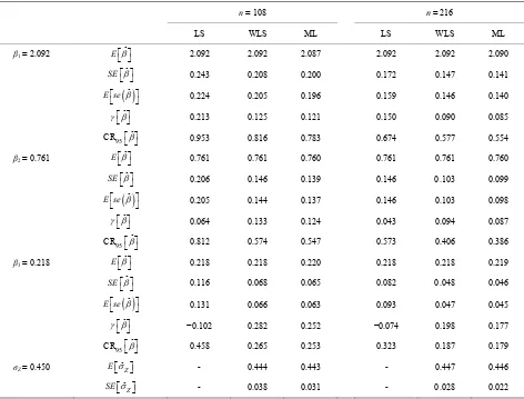
Table 2. The expected value (E[–]), standard errors (SE[–], E[se(–)]) , skewness (γ[–]) and CR95 for the estimates of βa.

n = 108 n = 216

LS WLS ML LS WLS ML

β1 = 2.092 E _{ }ˆ 2.092 2.092 2.087 2.092 2.092 2.090

ˆ

SE _{ } 0.243 0.208 0.200 0.172 0.147 0.141

 

ˆ E se  

 

ˆ

0.224 0.205 0.196 0.159 0.146 0.140

  _{ }

95 ˆ CR

0.213 0.125 0.121 0.150 0.090 0.085

    

β2 = 0.761 E ˆ

0.953 0.816 0.783 0.674 0.577 0.554

    

ˆ SE

0.761 0.761 0.760 0.761 0.761 0.760

  

  0.206 0.146 0.139 0.146 0.103 0.099

 

ˆ E se  

 

ˆ

0.205 0.144 0.137 0.146 0.103 0.098

  _{ }

95 ˆ CR

0.064 0.133 0.124 0.043 0.094 0.087

    

β3 = 0.218 E ˆ

0.812 0.574 0.547 0.573 0.406 0.386

    

ˆ SE

0.218 0.218 0.220 0.218 0.218 0.219

  

  0.116 0.068 0.065 0.082 0.048 0.046

 

ˆ E se  

 

ˆ

0.131 0.066 0.063 0.093 0.047 0.045

  _{ } − −

95 ˆ CR

0.102 0.282 0.252 0.074 0.198 0.177

    

σZ= 0.450 ˆ

0.458 0.265 0.253 0.323 0.187 0.179

Z

E_ _

ˆ

- 0.444 0.443 - 0.447 0.446

Z

SE_ _ - 0.038 0.031 - 0.028 0.022

a_{Data were generated from Model B, 4 million iterations. For reference, the ss of the al distribution is γ , whereas t -normal d y···y}

n

from Model B has skewness γ = 1.53.

skewne norm = 0 he log ata 1

Figure 2. The SE_μˆ X=x0_ and Ese



μˆ X=x0



 for

s, ap ed from Model A

ed on s with sample size

n = 108.

0

LS-estimates produced an α* _{which was much smaller} than α (α* _{< 0.2α, regardless of H}

1). This was a result of on of SE ˆ

. the three method

Results were bas

plied to data generat 4 million iteration

For a model with no intercept (β = 0), tests of the

the overestimati   0 by se

 

ˆ0 . For tes

be

ts of WLS- and ML-estimates, α* _{was approximately equal to} α (within 10% of the true value). A slight skewness could

observed; α*_{≤ α for H}

1: β0 > 0 and α*≥ α for H1:β0 < 0, while α* _{for H}

1:β0≠ 0 was slightly higher or the same as α. The source of this skewness was a positive correla-

ˆ

tion between 0 and se

 

ˆ0 ; small values of ˆ0 gave more extreme (negative) test-scores. For a model

e om Mo sis

where X has no effect on Y (β1 = 0), all three tests pro- duced α*_{-values close to α (within 20% of the true value).} For ML, α* _{was slightly higher than for LS and WLS.} The risk of type I error was approximately the same even when the sample size was doubled (n = 216).

Data were gen rated fr del A and the hypothe

H0:βi = βT was tested (βT was the parameter value speci-

fied in Model A). The results for WLS and ML (data not shown) were that α* _{was within 30% and 16% of α, re-}

[image:7.595.58.285.494.678.2]

spectively for nominal size 0.05 and 0.10. For nominal size 0.01 the relative deviation could be up to 70%. As before, tests of the LS-estimates of β0 prod

uch too small (α* _{≤ 0.1α). Both WLS- and ML-pro-} duced a slight skewness regarding tests of both β0 and β1, similar to that in Table 3.

Data were also generated according to Model B (data uced an α* m

ˆ

i SE

not shown) and the hypothesis H0:βi= βT was tested. For

all three methods, α* _{was closest to α for nominal size} 0.10. The relative deviation was largest for nominal size 0.01; 0.7α ≤ α* _{≤ 2.2α. Again, a skewness (as above)} could be seen in the tests of all three parameters, caused by the negative skewness of the test statistics. For tests of

the LS-estimate of β1, α* was consistently too large (1.04α ≤ α* _{≤ 2.20α), whereas α}* _{was consistently too} small in tests of β3 (0.30α ≤ α*≤ 0.76α). These erroneous risks were, again, the result of under- and overestimation, respectively, of  

 

ided and one-sided tests regarding β0 and β1a.

α = 0.050 α = 0.100

, see Table 2. Tests regarding the LS-estimates of β2 followed the same pattern as the tests of all the WLS- and ML-estimates. The risk of type I error was approximately the same even when the sam- ple size was doubled (n = 216).

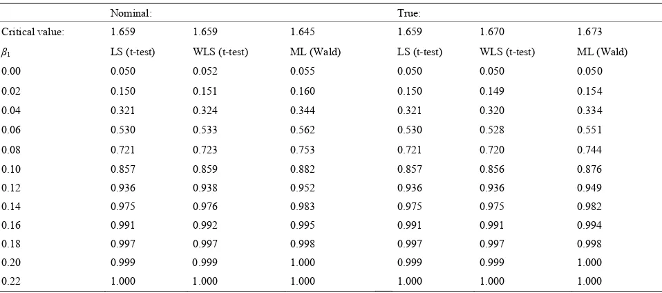
[image:8.595.55.540.272.468.2]

The power of the tests, under the alternative hypothe- sis H1:β1 > 0, was estimated for both α = 0.05 and α* = 0.05, see Table 4. When α = 0.05, ML had the highest power while LS had the lowest. For LS the type I error

Table 3. Risk for type I error (α*

) for two-s

α = 0.010

Alternative hypothesis H1: βi ≠ 0 βi < 0 βi > 0 βi ≠ 0 βi < 0 βi > 0 βi ≠ 0 βi < 0 βi > 0

βi n Test

β0 108 LS t-test 0.000 0.000 0.000 0.001 0.001 0.003 0.004 0.007 0.016

108 WLS t-test 0.010 0.012 0.008 0.051 0.055 0.047 0.102 0.106 0.096

108 M 0.106 0.100

216 S t-test 0.000 0.000 0.001 0.003 0.003 0.007 0.014 L Wald 0.012 0.013 0.010 0.054 0.056 0.050 0.106

L 0.000 0.001

216 WLS t-test ML W

0.010 0.011

0.011 0.012

0.009 0.009

0.050

0.052 0.053 0.049

0.053 0.047 0.100

0.102 0.103

0.104 0.097 0.099 216 ald

β1 108 LS t-test 0.010 0.010 0.010 0.050 0.050 0.050 0.100 0.101 0.100

108 WLS t-test 0.011 0.011 0.010 0.052 0.051 0.051 0.102 0.102 0.101 108 ML Wald 0.012 0.012 0.011 0.055 0.053 0.053 0.106 0.104 0.103 216 LS t-test 0.010 0.010 0.010 0.050 0.050 0.050 0.100 0.100 0.100 216 WLS t-test 0.010 0.010 0.010 0.051 0.050 0.051 0.101 0.100 0.101 216 ML Wald 0.011 0.011 0.011 0.052 0.051 0.052 0.103 0.101 0.102

a_{D re rated odel e β}

i= stim re b illio ons nc

owe ests lter y is H1: he risk of type I er t a.

Nomin True:

[image:8.595.59.538.505.717.2]

ata we gene from M A wher 0 and e ations a ased on 4 m n iterati with bala ed data.

Table 4. The p r for t with a native h pothes β1 > 0 w re the ror is se to 0.05

al:

Critical value: 1.659 1.659 1.645 1.659 701.6 1.673

β - -tes ald) LS LS -te ald

50 0.050

0.04

.06 .533 .562 .528 .551

0

1 LS (t test) WLS (t t) ML (W (t-test) W (t st) ML (W )

0.00 0.050 0.052 0.055 0.050 0.0

0.02 0.150 0.151 0.160 0.150 0.149 0.154

0.321 0.324 0.344 0.321 0.320 0.334

0 0.530 0 0 0.530 0 0

0.08 0.721 0.723 0.753 0.721 0.720 0.744 0.1 0.857 0.859 0.882 0.857 0.856 0.876 0.12 0.936 0.938 0.952 0.936 0.936 0.949 0.14 0.975 0.976 0.983 0.975 0.975 0.982 0.16 0.991 0.992 0.995 0.991 0.991 0.994 0.18 0.997 0.997 0.998 0.997 0.997 0.998 0.20 0.999 0.999 1.000 0.999 0.999 1.000 0.22 1.000 1.000 1.000 1.000 1.000 1.000

a _{ere generated from with diff lues but cons 4.804. Estim io ased on 1 m rations with ba ata and sam-} ple size n = 108.

r as correct but LS and ML the critical v were adjusted to g = 0.05. adjustment still had the highest r while WLS now had a l p r compared to LS. The relative difference bet th ominal and tru for β1 = 0 decreases with β1.

similar to the geometric mean expo- sure (0.345 against 0.386). Thus the data can be consid-

mod wood-fire or been in a residence

ods sh w ignifican rence betwe

the LS LS-regr models o othenburg differe indesbe the ML-re on model

also sh w rence betw almo and

Lindesber = 0.041). the ML-re n model showed a significantly lo posure fo smokers

In

ation is often used to stabilize the variance, but this distorts the linear relationship and does not give

absolute effect of a predictor.

isk w for W alues

ive α* _{After ML}

powe ower

owe ween

e n e power was largest and

4.4. Application: 1,3-Butadiene Exposure in Five Swedish Cities

The data on 1,3-butadiene were found to be highly skewed (γ = 2.764) whereas the log-transformed values were approximately symmetrical (γ = 0.279). The me- dian exposure was

ered log-normal. Five predictors were included in the el: “Have you lit a

heated with wood burning?” (Wood burning, yes/no), “Are you a smoker?” (Smoker, yes/no), “Have you been in an indoor environment where people where smoking?” (ETS, yes/no), “Proportion of time spent in traffic?” (Traffic), and “City of residence”: Umeå (Ume), Stock- holm (Sthlm), Malmö (Malmo), Gothenburg (Gbg), and reference category Lindersberg. These predictors had been shown to be significant in previous studies on other datasets [15-17].

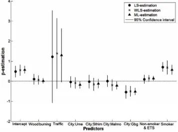
Neither Woodburning nor Traffic were significant in any of the regression models (for ML Traffic was bor- derline significant, p = 0.059), Figure 3. All three meth-

o ed a s t diffe en the cities; in

- and W ession nly G

d from L rg, but gressi o ed a significant diffe een M

g (p Only

wer ex

gressio r

non-with no ETS (p = 0.013). There were clear differences in range of the confidence intervals; with one exception ML had the narrowest intervals and LS the widest.

A second analysis with only the non-smokers (n = 225) was performed and then Traffic became significant in the ML-regression model (p = 0.039). Otherwise the same predictors were significant in all three analyses, as for the full dataset.

5. Discussion

this study a new maximum likelihood-based method for estimating a linear regression model for log-normal heteroscedastic data was evaluated and compared with two least squares methods. For log-normal data, the log-transform

an estimate of the

Our simulation study demonstrated that the new maximum likelihood method (ML) provides unbiased estimates of the regression parameters βi, and so do the

[image:9.595.119.476.444.709.2]

least squares method (LS) and the weighted least squares method (WLS).

Figure 3. The LS-, WLS- and ML-estimations of the predictor effects, βi, and their 95% confidence intervals (CI) for regression analysis with 1,3-butadiene as the response.

One reason for proposing a new regression method is the need for a method to estimate a linear regression in the presence of heteroscedasticity. The effect of ignoring the increasing variance is demonstrated in the use of LS, where the standard error, SE  ˆi , was up to 78% larger

than that e examples that were investigated. Since the heteroscedasticity of the data was ignored when using LS, the confidence interval was too wide. The results of our example with 1,3-butadiene data were consistent with those in the simulation study; LS overall had the widest confidence intervals and ML the narrow- est for the predictor effects.

For all three methods, estimates of the expected re- sponse,

of ML, for th

ˆ_{Y X}

μ , were unbiased. The confidence interval for ˆμ_{Y X} is based on se

 

μˆ_{Y X} , which depends on the value of t x0. For a model with one predictor, both ML produced an almost correct confi- dence in the narrowest interval at

he predictor, and WLS terval, with 0 0,1

x  SE ˆ0 SE ˆ1, whereas LS had its nar- at

  

rowest confidence interval    x0 X which therefore nfidence intervals.

For ML and WLS the sample-specific standard error, does produce erroneous co

 

ˆ

i

se  , was a good estimator of the true standard error, hereas for LS,



w se ˆ0



greatly overestimated SE  ˆ0 . When investigating the true risk of type I error, α*_{, for} tests regarding the regression parameters, the t-tests of the LS-estimates of the intercepts produced an α* _much smaller than the nominal α. This was a consequence of the too large se

 

ˆ0 , c he distribution of the t-statistics to have fewer observations in the tails than expected. For both the Wald-test (ML) and the t-test used for the WLS-estimates, the α* _{was approximately equal} to α (for nominal size {0.01, 0.05, 0.10} the largest rela- tive deviations were α* _{= {0.021, 0.072, 0.125}). For all} three methods, the relative deviation (

ausing t

*

 ) was largest at nominal size 0.01, indicating a skewness of the test st

both reg inal

atistics in the tails. Regarding the power (in tests of β1), ML was superior to LS, arding the true and nom power.

The precision of an estimated expected value ( ˆμ_{Y X}) depends both on the regression method and on the varia- tion of the predictors X1, ,  Xp. If a predic

he estimated effect of that predictor will have a large stand or. In some situa- tions a better estimation of the exposure might

tor has a

very sm n t

ard err

be achieve with

variatio

egressi he expo

models can also be used to estimate the exposure for a whole population, provided that the distribution of the background factors is known.

When investigating an exposure-disease associations, the measured exposure sometimes include a stochastic error (exposuremeasured = exposuretrue + error1), which is unrelated to the stochastic error of the (linear) expo- sure-response model (response = δ0 + δ1·exposure + er-

ror2). The issue with regression analysis where the ex- planatory variable has measurement errors is raised in [23]; given the true exposure, the measured exposure has a stochastic variation and different approaches to esti- mating the true exposure are compared. In situations with measurement errors, the individual- and group-based exposure assessment approaches are often compared, see e.g. [24,25]. In an individual-based approach, each per- son’s measured exposure is used which often leads to a bias of δ1 towards null. In a group-based approach, each person is assigned an exposure based on group affiliation, which is the same as estimating the exposure from a re- gression model with only one explanatory variable,

Group. If several relevant explanatory variables are used

ased ap

re-re-

di all variation, the

a model that excludes predictors with very small n, as has been investigated in [22] for a situation where land-use r on is used to estimate t - sure. Apart from effect estimation, regression analysis can be used to estimate the expected value of the re- sponse variable given certain values of the background factors (e.g. to estimate the personal exposure as a func- tion of easily measured background factors). Regression

an individual-b proach. A group-based design of ten leads to errors in the exposure which are of Berk- son-type (exposuretrue = exposuregroup + error3), or ap- proximately Berkson-type. As discussed in [24], in a true Berkson-error-model, the error3 is independent of expo-

suregroup, whereas the approximate Berkson-error may depend of the group size. The approximate Berkson-error is, however, independent of error2. A group-based ap- proach often leads to less bias in the δ1 estimate but a larger standard error, see e.g. [24,26]. A group-based approach with a log-linear exposure-response model can have a substantial b

to estimate the exposure (rather than only Group) the standard error will decrease and, thus, be more similar to

ias in the estimated exposu sponse effect [27].

of data sets would be needed.

In the simulation study, data were generated from a log-normal heteroscedastic distribution with certain pa- rameter values. However, empirical data might be only approximately log-normal and thus exhibit a larger vari- ance than the one in a perfect log-normal distribution. Thus the results from the simulation study might not hold completely for real data sets of e.g. exposure data. Also, in the simulation study the predictors were assumed to be measured without measurement errors which might be unrealistic for some predictors. Therefore, evaluation of the new ML method should also be made on several em- pirical data sets.

Two specific simulation models were used in this study where the parameters were estimated from an em- pirical dataset and therefore the simulation models can be considered to be fairly realistic. The results on bias and standard error are likely to be valid also in models with other parameter values. The parameter estimates are un- biased both for a simple model (with intercept and one explanatory variable) and for a model with three ex- planatory variables and no intercept, and in both situa- tions ML gives the smallest standard errors. This sug- gests that the results can be generalized to other datasets.

The ML estimates are derived true iterations and in some situations (sometimes caused by unsuitable start values or large variance in the data) the iterations don’t converges. This may lead to unrealistic estimations. In those cases, censoring data larger than the 95% quantile will stabilize the results but will cause underestimations of the intercept and standard errors. In those situations WLS will generally give the best result.

In this study the methods have been evaluated for rela- tively large samples (n = {108, 216}) and the conclusion was that the asymptotic properties of maximum likely- hood estimates are valid for these sample sizes. However, for smaller samples, further evaluation is needed, espe- cially regarding the distribution of the estimates. In other studies regarding smaller samples of untransformed log- normal data, likelihood-based approaches has been sug- gested for constructing confidence intervals for the mean and mean response [28,29].

This study illustrated that the new maximum likely- hood-based regression method has good properties and can be used for linear regression on log-normal hetero- scedastic data. It provides an estimate of the absolute effect of a predictor, while taking the increasing variance into account in an optimal way. The study also demon- strated that the results from the weighted least squares regression (where the increasing variance is accounted for) were very similar to those from the ML method. Al- though ML gave slightly narrower confidence intervals and had higher power regarding β1, both WLS and ML can be recommended for linear regression models for

log-normal heteroscedastic data.

6. Acknowledgements

We would like to thank Urban Hjort for sharing his MATLAB codes for the regression analysis.

REFERENCES

[1] P. O. Osvoll and T. Woldbæk, “Distribution and Skew- ness of Occupational Exposure Sets of Measurements in the Norwegian Industry,” Annals of Occupational Hy- giene, Vol. 43, No. 6, 1999, pp. 421-428.

[2] K. M. McGreevy, S. R. Lipsitz, J. A. Linder, E. Rimm and D. G. Hoel, “Using Median Regression to Obtain Adjusted Estimates of Central Tendency for Skewed Laboratory and Epidemiologic Data,” Clinical Chemistry, Vol. 55, No. 1, 2009, pp. 165-169.

doi:10.1373/clinchem.2008.106260

[3] R. Branham Jr, “Alternatives to Least Squares,” The As- tronomical Journal, Vol. 87, 1982, pp. 928-937.

doi:10.1086/113176

[4] A. C. Olin, B. Bake and K. Toren, “Fraction of Exhaled Nitric Oxide at 50 mL/s—Reference Values for Adult Lifelong Never-Smokers,” Chest, Vol. 131, No. 6, 2007, pp. 1852-1856. doi:10.1378/chest.06-2928

[5] J. O. Ahn and J. H. Ku, “Relationship between Serum Prostate-Specific Antigen Levels and Body Mass Index in Healthy Younger Men,” Urology, Vol. 68, No. 3, 2006, pp. 570-574. doi:10.1016/j.urology.2006.03.021

[6] L. Preller, H. Kromhout, D. Heederik and M. J. Tielen, “Modeling Long-Term Average Exposure in Occupa- tional Exposure-Response Analysis,” Scandinavian Jour- nal of Work, Environment & Health, Vol. 21, No. 6, 1995, p. 8. doi:10.5271/sjweh.67

[7] M. Watt, D. Godden, J. Cherrie and A. Seaton, “Individual Exposure to Particulate Air Pollution and Its Relevance to Thresholds For Health Effects: A Study of Traffic War- dens,” Occupational and Environmental Medicine, Vol. 52, No. 12, 1995, pp. 790-792.

doi:10.1136/oem.52.12.790 [8]

, pp. 6072-6092. doi:10.1002/sim.3427

B. Dickey, W. Fisher, C. Siegel, F. Altaffer and H. Azeni, “The Cost and Outcomes of Community-Based Care for the Seriously Mentally Ill,” Health Services Research, Vol. 32, No. 5, 1997, p. 599.

[9] R. Kilian, H. Matschinger, W. Loffler, C. Roick and M. C. Angermeyer, “A Comparison of Methods to Handle Skew Distributed Cost Variables in the Analysis of the Resource Consumption in Schizophrenia Treatment,” Journal of Mental Health Policy and Economics, Vol. 5, No. 1, 2002, pp. 21-32.

[10] J. P. T. Higgins, I. R. White and J. Anzures-Cabrera, “Meta-Analysis of Skewed Data: Combining Results Re- ported on Log-Transformed or Raw Scales,” Statistics in Medicine, Vol. 27, No. 29, 2008

L. Hui, “Methods for Compar- ing the Means of Two Independent Log-Normal Sam- [11] X.-H. Zhou, S. Gao and S.

ples,” Biometrics, Vol. 53, No. 3, 1997, pp. 1129-1135. doi:10.2307/2533570

[12] T. H. Wonnacott and R. J. Wonnacott, “Regression: A Second Course ew York, 1981. [13] Y. Yurgens, “ tal Impact by

Log-r, L. Barregard

s.7500562 in Statistics,” Wiley, N Quantifying Environmen

Normal Regression Modelling of Accumulated Expo- sure,” Licentiate of Engineering, Chalmers University of technology and Göteborg University, Gothenburg, 2004. [14] S. Johannesson, P. Gustafson, P. Molna

and G. Sallsten, “Exposure to Fine Particles (PM2.5 and PM1) and Black Smoke in the General Population: Per- sonal, Indoor, and Outdoor Levels,” Journal of Exposure Science and Environmental Epidemiology, Vol. 17, No. 7, 2007, pp. 613-624. doi:10.1038/sj.je

E. Jenkin, “Ambient [15] G. J. Dollard, C. J. Dore and M.

Concentrations of 1,3-Butadiene in the UK,” Chemico- Biological Interactions, Vol. 135-136, 2001, pp. 177-206. doi:10.1016/S0009-2797(01)00190-9

[16] Y. M. Kim, S. Harrad and R. M. Harrison, “Concentra- tions and Sources of VOCs in Urban Domestic and Public Microenvironments,” Environmental Science & Technol- ogy, Vol. 35, No. 6, 2001, pp. 997-1004.

doi:10.1021/es000192y

[17] P. Gustafson, L. Barregard, B. Strandberg and G. Sallsten, “The Impact of Domestic Wood Burning on Personal, Indoor and Outdoor Levels of 1,3-Butadiene, Benzene, Formaldehyde and Acetaldehyde,” Journal of Environ- mental Monitoring, Vol. 9, No. 1, 2007, pp. 23-32. doi:10.1039/b614142k

[18] U. Bergendorf, K. Friman and H. Tinnerberg, “Cancer- Framkallande ämnen i Tätortsluft-Personlig Exponering och Bakgrundsmätningar i Malmö 2008,” Report to the Swedish Environmental Protection Agency Department of Occupational and Environmental Medicine Malmö, 2010.

[19] W. H. Greene and C. Zhang, “Econometric Analysis,” Vol. 5, Prentice Hall, Upper Saddle River, 2003.

nd

[20] J. Hass, M. D. Weir and G. B. Thomas, “University Cal- culus,” Pearson Addison-Wesley, 2008.

[21] Y. Pawitan, “In All Likelihood: Statistical Modelling a Inference Using Likelihood,” Oxford University Press, Oxford, 2001.

[22] A. A. Szpiro, C. J. Paciorek and L. Sheppard, “Does More Accurate Exposure Prediction Necessarily Improve Health Effect Estimates? [Miscellaneous Article],” Epi- demiology, Vol. 22, No. 5, 2011, pp. 680-685.

doi:10.1097/EDE.0b013e3182254cc6

[23] Y. Guo and R. J. Little, “Regression Analysis with Co- variates That Have Heteroscedastic Measurement Error,” Statistics in Medicine, Vol. 30, No. 18, 2011, pp. 2278- 2294. doi:10.1002/sim.4261

[24] H. G. M. I. Kim, D. Richardson, D. Loomis, M. Van Tongeren and I. Burstyn, “Bias in the Estimation of Ex- posure Effects with Individual- or Group-Based Exposure Assessment,” Journal of Exposure Science and Environ- mental Epidemiology, Vol. 21, No. 2, 2011, pp. 212-221. doi:10.1038/jes.2009.74

[25] S. Rappaport and L. Kupper, “Quantitativ sessment,” Stephen Rapp

e Exposure As- aport, 2008.

and S. Zhao, “Biases in Es- [26] E. Tielemans, L. L. Kupper, H. Kromhout, D. Heederik and R. Houba, “Individual-Based and Group-Based Oc- cupational Exposure Assessment: Some Equations to Evalu- ate Different Strategies,” The Annals of Occupational Hygiene, Vol. 42, No. 2, 1998, pp. 115-119.

[27] K. Steenland, J. A. Deddens

timating the Effect of Cumulative Exposure in Log-Lin- ear Models When Estimated Exposure Levels Are As- signed,” Scandinavian Journal of Work Environment & Health, Vol. 26, No. 1, 2000, pp. 37-43.

doi:10.5271/sjweh.508

[28] J. Wu, A. C. M. Wong and G. Jiang, “Likelihood-Based

-1860. Confidence Intervals for a Log-Normal Mean,” Statistics in Medicine, Vol. 22, No. 11, 2003, pp. 1849

doi:10.1002/sim.1381