Design studies of model reference adaptive control and identification systems

warwick.ac.uk/lib-publications

A Thesis Submitted for the Degree of PhD at the University of Warwick

Permanent WRAP URL:

http://wrap.warwick.ac.uk/97572

Copyright and reuse:

This thesis is made available online and is protected by original copyright.

Please scroll down to view the document itself.

Please refer to the repository record for this item for information to help you to cite it.

Our policy information is available from the repository home page.

STATEMENT

The work presented in this Thesis has not been submitted

for another degree of this or any other University. It is original

with the exceptions stated below:

(i) The work in Chapter 1 is a review and commentary on the existing

design methods for model reference adaptive systems.

(ii) In Chapter 2, the performance comparison of M.I.T. and Liapunov

designs with step and sinusoidal inputs was reported in the candidate's

M.Sc. dissertation. This work is reproduced here for the sake of

completeness. The performance study for stochastic inputs and the

inclusion of three other designs are new.

(iii) Elsewhere in the thesis ideas, results and examples which are

due to other authors are clearly acknowledged in the references.

ABSTRACT

This thesis sets out to compare five well known design rules

for the design of model reference adaptive systems. These are the

M.I.T. rule, the Liapunov synthesis, the gradient rules of Dressier

and Price, and the Monopoli design rule. A systematic performance

comparison is made using two low order gain adjustment systems

simulated on a digital computer. Step, sinusoidal and stochastic

input signals are used and the system state variables and performance

criteria are all expressed as dimensionless quantities. The results

clearly demonstrate the superior performance of the Liapunov and

Monopoli designs. The main disadvantage of other designs is that the

dimensionless performance criteria is not a monotonic decreasing

function of the dimensionless gain parameter. An analysis of the

noisy case is then performed and this further points out the flexibility

of the Liapunov synthesis.

The next objective of the research is to extend the scope of

application of the Liapunov designs. First a modification of the usual

design algorithm for multivariable systems is made sc that a wider

class of plants, in which the adjustable parameters may appear simul­

taneously in two or more elements of the plant and control matrices,

can be readily treated. Examples are given to illustrate the design

procedures and the typical performance of such designs. Secondly, the

simultaneous parameter and state estimation system using model

reference methods is investigated. Landau's hyperstability design,

which can be shown to be equivalent to the Liapunov design, is preferred

for this problem. To distinguish this design from the well known

Generalized Equation Error (G.E.E.) design, we have called it the

Stable Response Error (S.R.E.) design. The practical difficulty of

using this globally stable design rule is found to be the implementation

of the series (derivative) compensator. It is then shown how the

problem is solved by using the state variable filters. Various

simulation results substantiate the characteristics (namely unbiased

estimates and very fast convergence) of the resulting design. The

recovery of the simultaneous state estimates when the state variable

filters are used with the S.R.E. design is then considered. With

a moderate rate of convergence, the quality of the state estimates is

found to be good. The main disadvantage of the S.R.E. method is that

the range of parameter variations must be known a priori in order to

design the series compensator which ensures the global stability.

Finally, the extensions of the S.R.E. method to treat nonlinear and

multivariable systems are presented. The main effort here is to

find the appropriate structures of the estimation model.

To conclude the thesis, a real case study is presented.

This is the modelling of a nonlinear, third order internal combustion

engine by a linear, first order model. The parameters of the model

are adjusted according to the S.R.E. design rule. The practical

results obtained demonstrate the feasibility of using the model

reference method in a real physical system. Then some of the

experiments are repeated with the estimation system based on the

G.E.E. design rule. The results are found much inferior to those

ACKNOWLEDGEMENTS

The author wishes to express his deepest gratitude to

Professor P.C. Parks who supervised this research work, for his

guidance and encouragement throughout its progress. He is also

indebted to The Royal Commission For The Exhibition of 1851, for

the financial assistance in the form of an Overseas Scholarship,

and to the British Cov.cil, for the granting of a Fees Award. Thanks

are also due to Professor R.V. Monopoli (University of Massachusetts),

Professor I.D. Landau (ALSTHOM Research Laboratory and University

of Grenoble) and Professor J.L. Douce (University of Warwick) for

their encouragement and many useful discussions. Finally, his

thanks go to his colleague, Mr. J.N. Devlukia, for his assistance

in the experiments on the internal combustion engine and to Mrs.

V. Carroll for her patience in typing this thesis.

Y

LIST OF CONTENTS

Page N o .

CHAPTER 1 - INTRODUCTION

1.1 BACKGROUND INFORMATION 1

1.2 LITERATURE SURVEY 2

1.2.1 Adaptive Control 2

1.2.2 Identification 5

1.3 PURPOSE AND LAYOUT OF THE THESIS 8

1.4 DEFINITIONS AND THEOREMS 10

CHAPTER 2 - COMPARATIVE STUDIES OF MODEL REFERENCE

ADAPTIVE CONTROL (M.R.A.C.) SYSTEMS

2.1 INTRODUCTION 15

2.2 A CRITICAL COMPARISON OF THE DESIGN RULES 17

2.2.1 M.I.T. Rule and Liapunov Synthesis 17

2.2.2 Other Design Rules 21

2.2.3 A Simulation Study of the Adaptive 23

Response

2.3 A SYSTEMATIC PERFORMANCE COMPARISON 25

2.3.1 First Order Systems 26

2.3.2 Second Order Systems 33

2.3.3 Summary 38

2.4 GENERAL DISCUSSIONS 39

2.4.1 General Parameter Adjustments 39

2.4.2 Eftects of Noise 41

2.4.3 Noise and Disturbance Rejection 43

2.5 CONCLUSIONS - 44

(v)

CHAPTER 3 - DESIGN OF MULTIVARIABLE M.R.A.C. SYSTEMS

USING LIAPUNO.’ SYNTHESIS

3.1 INTRODUCTION

3.2 GENERAL DESIGN ALGORITHM PREVIOUSLY

SUGGESTED

3.3 A MORE GENERAL DESIGN ALGORITHM

3.4 AN ILLUSTRATIVE EXAMPLE

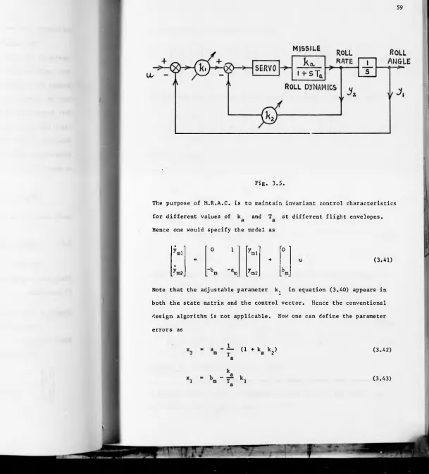
3.5 FURTHER EXAMPLES

•3.6 CONCLUSIONS

CHAPTER 4 - DESIGN OF MODEL REFERENCE PARAMETER AND

STATE ESTIMATION SYSTEMS

4.1 INTRODUCTION

4.2 THE STABLE RESPONSE ERROR (S.R.E.) METHOD

FOR PARAMETER ESTIMATION

4.2.1 Statement of the Basic Problem

4.2.2 The Basic Design Rule

4.2.3 The Role of the Proportional (Feed­

forward) Loops

4.2.4 The State Variable Filters

4.2.5 Noise Contamination

4.2.6 Simulation Results

4.3 THE ADAPTIVE STATE OBSERVER

4.3.1 Development

4.3.2 Simulation Results

4.4 EXTENSIONS

4.4.1 A Class of Nonlinear Plants

4.4.2 A Class of Multivariable Systems

CHAPTER 5 - AN APPLICATION CASE STUDY

5.1 INTRODUCTION 98

5.2 A BRIEF DESCRIPTION OF THE SYSTEM AND 99

THE EXPERIMENTS

5.2.1 The Engine 99

5.2.2 The Experimental Setup 100

5.2.3 The Adaptive Models 102

5.3 EXPERIMENTAL RESULTS 104

5.3.1 The S.R.E. Design 104

5.3.2 The G.E.E. Design 111

5.4 CONCLUDING REMARKS 114

CHAPTER 6 - FINDINGS AND FURTHER WORK 115

6.1 FINDINGS 115

6.2 SUGGESTIONS FOR FURTHER WORK 117

REFERENCES 119

APPENDICES

A.l. Liapunov Design 125

A. 2. Differential Equations of the Various 127

Designs

A. 3. Dimensional Analysis 129

A.4. The Stochastic Signal 131

A. 5. The Adaptive Laws for General Parameter 136

Adjustments

A.6. Hyperstability and Identification 138

A.8. Parameter Sensitivity of Positive

Real Functions

A.9. The Generalized Equation Error Method

A.10. Transformation to a Canonical Form

CHAPTER 1 INTRODUCTION

1.1. BACKGROUND

The model reference adaptive control (M.R.A.C.) technique

has been a popular approach to the control of systems operating in the

presence of parameter and environmental variations. In such a scheme,

the desirable dynamic characteristics of the plant are specified in

the reference model and the input signal or the controllable parameters

of the plant are adjusted, continuously or discretely, so.that its

response will duplicate that of the model as closely as possible. The

identification of the plant dynamic performance is not necessary and

hence a fast adaptation can be achieved.

In the last decade or so, the design methods for M.R.A.C.

systems have been dominated by the so called M.I.T. rule and many

attempts have been reported to implement the resulting design in real

physical systems. However, more often than not, the designer finds

himself confronted with a complex stability problem or inadequate

performance of the adaptive loop and all these limit the widespread

application of M.R.A.C. techniques although it is thought to be an

attractive alternative to many conventional methods. In the same

period, other new design methods have been developed to overcome the

snortcomings of the M.I.T. rule and the literature is flooded with new

proposals. In fact the situation has reached a stage where the

designer is fairly confused about the status of the various methods

now available.

Recently tho concept of model reference has been regarded

more generally than it was first being used for in adaptive control.

For instance, it can be readily shown that the well known Kalman

of parallel model reference systems. Two important methods of system

identification namely the equation error method and the response error

method can be formulated as a series-parallel and parallel model

reference systems respectively. Also the recently popularized method

of compensating multivariable systems, namely the model following method,

can be treated as a parallel model reference system. Hence, further

research on M.R.A.C. systems will benefit all these important areas of

automatic control.

It is with such a background that this research has been

initiated. It does not attempt to invent entirely new design rules.

Rather the main effort has been expanded on the clarification of the

status of the art of designing model reference adaptive systems and on

further development of some prospective design rules to simplify the

implementation and to widen the scope of their application.

1.2. LITERATURE SURVEY

1.2.1. Adaptive Control

The M.R.A.C. system was first designed by the performance

index minimization method proposed by Whitaker ^ of the M.I.T.

Instrumentation Laboratory and has since then been referred as the

M.I.T. design rule. The performance index is the integral squared of

the response error. This rule has been very popular due to the simplicity

in the practical implementation of the plant gain adjustment loop. For

the adjustment of other parameters, however, sensitivity filters are

required and the hardware involved may be prohibitive for simultaneous

multi-parameter adjustments. An improved design rule with respect to

3

the speed of response has then been proposed by Donalson who used a

more general performance index than that of Whitaker, but additional

need of the sensitivity filters can be avoided by a gradient method

developed later on by Dressier , or by an 'accelerated gradient method'

suggested by Price ^ . The latter is easier to implement and is

capable of achieving faster adaptations compared with other gradient

techniques. Another contribution to the simplification of the design

comes from the application of sensitivity analysis by Kokotovic et

7 8

al ’ resulting in a design similar to the M.I.T. rule. Here, with

further approximation, only one sensitivity filter is required for

simultaneous multi-parameter adjustments. For some other particular

. 27

applications, W m s o r has also modified the M.I.T. rule to reduce

the sensitivity of the response to the loop gain, at the expense of

additional instrumentation. All the design rules mentioned are not

however, globally stable and hence the adaptive gain which governs the

speed of response is limited. A good compromise between the stability

and the speed of adaptation will have to be decided by laborious

simulation studies. A recent contribution by Green ** has extended the

work of Dressier to form a 'stable maximum descent' method. However

this adaptive rule is not attractive from a practical viewpoint because

the first derivatives of the state vectors are often required to assure

global stability of the resulting system.

Owing to the serious problem of instability encountered in

the M.I.T. rule and other gradient techniques, two branches of research

have become very active. These are the theoretical stability analysis

using such tools as the second method of Liapunov, and the new synthesis

approach which avoids the instability problem. The effort in the

analysis of the parameter adjustment loops,^which differential equations

24

arc nonlinear and nonautonomous, are summarized by James who shows

that the current status of control theory can only cope with simple

systems with deterministic signals and can hardly treat those with

and time consuming. On the other hand, in the Liapunov synthesis

approach, the adaptive rule is obtained by selecting the design equations

to satisfy conditions derived from the second method of Liapunov, so that

the system stability is guaranteed for all inputs. Butchart and

9

Shackcloth have first suggested the use of a quadratic Liapunov

• . 2

function which was employed later on by Parks to redesign systems

formerly designed by the M.I.T. rule. The use of a different Liapunov

.

.

function by Phillipson and Gilbart et al has resulted in the

introduction of proportional (feedforward) loops which would improve

the damping of the adaptive response.

The main disadvantage of the Liapunov method is that the entire

state vector must be available for measurement, which is not often

possible. Recent efforts in the application of the idea of positive real

13 14

transfer function, notably that by Monopoli * , have allowed one to

eliminate or reduce the number of differentiators required to implement

the design rule for adjusting both the plant gain and other parameters.

Among other possible solutions to avoid the use of derivative networks,

Currie and Stear have envisaged the use of a Kalman filter, which

would also handle the measurement noise problem, while the use of state

observers ^ to estimate the states of an unknown time-varying plant is

still an open question. Some recent contributions on adaptive state

17 18

observers ’ represent the serious interest and the early stage of

development in the use of observers in adaptive control. Another

limitation of the Liapunov design rule is that it may not be applicable to

cases where the plant parameters cannot be directly adjusted. Such a

case was mentioned by Winsor and Roy ^ but a solution has been found

14

.

.

.

recently by Monopoli . A further possibility of indirectly controlling

the plant by adjusting the feedforward and feedback gains has been

investigated by Landau et al and Narendra et al

The Liapunov design can also be derived using the hyperstability

stability approach, the analysis of nonideal systems is very simple.

For instance the conditions for bounded-input bounded-output stability

can be readily written down when noise or time-varying parameters are

present. Although the hyperstability approach could give many other

designs, so far the best found is still the same as the Liapunov design.

Hence besides the convenience in analysis the hyperstable design rule

is equivalent to the Liapunov design rule.

Other less well known but important designs deserve mentioning

25

here. Nikiforuk anc Rao have suggested combining the advantages of

the sensitivity and stability considerations and they produced an

adaptive rule which could be made stable if the bound on the parameter

26

variations is known. Choe and Hikiforuk have suggested a feedback

law which guarantees bounded-input bounded-output stability and uses

only partial state measurements. Both of these approaches use the

second method of Liapunov and represent alternative ways of designing

on the basis of stability theory. Finally, the readers are referred

27-29

to three recent survey papers for other proposed designs.

1.2.2. Identification

Process parameter estimation using an adjustable model has

39 A O

been a popular on-line system identification technique ’ . This

method seeks to adjust the parameters of the model contii.uously so as

to null some error measure between the plant and the model. Two types

of models have been widely used, one being the series-parallel model

28

while the other is the parallel model . The former yields an error

measure called the equation error which is linear in the unknown

parameters; the latter uses the response error as an error measure

which is non-linear in the unknown parameters. Hence they are also

seeks to minimize the square of error measure according to a steepest

41

descent law. It uses a so called state variable filter technique

to avoid pure signal differentiations and is proved to be globally

asymptotically stable. Recently the extension of this approach to

treat multivariable systems has been done by Pazdera and Pöttinger 49

50

Narendra and Kudva who use the Liapunov synthesis design rules,

61

and by Landau who uses the hyperstability design rule. The only

limitation of the G.E.E. method is that it gives biased estimates

when the plant output is corrupted by noise.

The parallel model approach is in fact the usual parallel

model reference adaptive system but with the adjustable model attempting

to track the stationary (or slow-varying) plant. Hence all that has

been said about the design methods in Section 1.2.1 may be applicable

here. The status of the design rules is as follows. The sensitivity

37 47

method ’ is most popular but uneconomical due to the large amount

of time-varying sensitivity filters required; the stability may be

52 4

assured in some designs . The gradient method of Dressier ,

Hsia and Vimolvanich does not require sensitivity filters but is

limited to local convergence only. The gradient method employing

52 .

stochastic approximation is stable but the amount of hardware

required for generating sensitivity functions is usually prohibitive

and the rate of convergence is very slow. The synthesis approach of

Parks ^ and Landau globally stable but its implementation

requires the use of the plant state vector. All these methods,

|

parallel model approach is that the former only gives parameter estimates

28 whereas the latter gives simultaneous parameter and state estimates

This aspect has not bean emphasized in the past primarily because the

latter was dominated by the sensitivity design rule which was difficult

to implement and because it was usually thought that the simultaneous

parameter and state estimation could be adequately handled by more

. 54 55

complex methods like the extended Kalman filter ’ . However it is

now well known that the extended Kalman filter possesses a serious

convergence problem and is also difficult to implement. The potential

of the parallel model reference techniques is its simplicity in structure

and. fewer apriori information about noise statistics. The assured

stability of the Liapunov and hyperstability designs will certainly

add to the attractiveness of using model reference systems for simultaneous

parame :er and state estimations.

With explicit parameter and state estimations, many well known

. . . 44,

control techniques can then be applied to achieve adaptive control

£ r £0

. Now there arises an important question as to when should M.R.A.C.

(without explicit identification) be used and when should the adaptive

control with on-line identification be used. Besides the usual

consideration about the accessibility of adjustable parameters, the

possibility of injecting test perturbations and the availability of

state vectors, the most important factor influencing the choice of

adaptive control technique is the question of whether or not the

plant has dominant right-half-plane zeros (nonminimum phase) which

vary with the operating condition. As the M.R.A.C. uses high gains

in the adaptive loops, it may not be suitable for systems with

nonminimum phase transfer function whereas the adaptive control employing

68

explicit identification can cope with this type of system . If the

8

as it avoids the usually difficult identification problems.

1.3. PURPOSE AND LAYOUT OF THF. THESIS

The initial part of this research is a continuation of work

done as an M.Sc. project in which a simulation study verified in some

examples the superior performance of the Liapunov design over the M.I.T.

rule. In this thesis, other gradient methods are included in the

comparison and more general stochastic inputs are also used. Only

continuous time linear models and plants are considered. The results

confirm the earlier observation that the Liapunov design possesses

excellent performance characteristics not attainable by other designs.

Hence further developments of the Liapunov design rule will be worth­

while in order to extend the usefulness of model reference techniques.

The latter part of the research thus includes the generalization of

the usual Liapunov design algorithm for multivariable systems to treat

a wider class of plants, the use of state variable filters for

implementing the parallel model reference identification system, and

a practical case study to assess the model reference systems designed

by using stability theories. The layout of the thesis is as follows.

Chapter 2 describes the comparative studies of several

design rules which include the M.I.T. rule, the Liapunov syntr.esis,

the gradient rules of Dressier and Price, and the. Monopoli design

rule. Step, sinusoidal and stochastic inputs are used in the systematic

performance comparison on the simulated examples. Dimensionless

variables and performance criteria are used so that the results are

most general. A qualitative analysis is then presented to discuss the

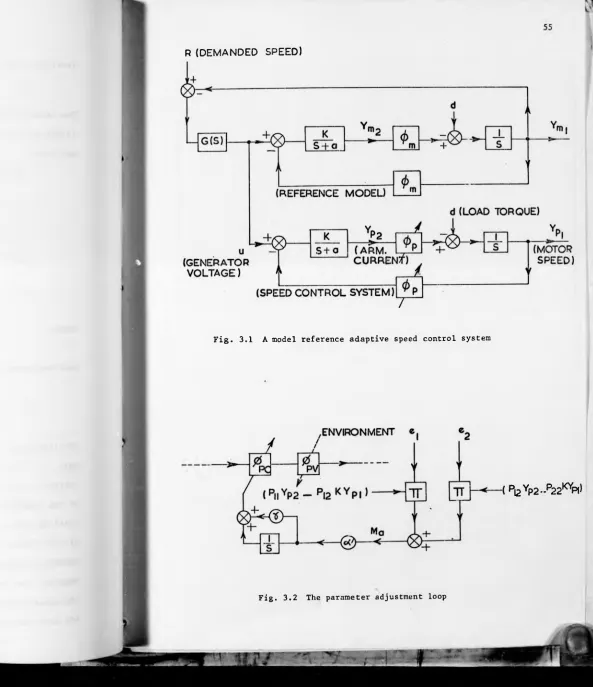
Chapter 3 reviews the commonly used Liapunov design algorithm

for the design of multivariable M.R.A.C, systems and points out its

limitation when used in some actual applications, A new general

algorithm is then derived and examined using the example of an

adaptive speed control loop for a Ward-I.eonard system. Qualitative

discussions of two more examples are also given.

Chapter 4 begins with the discussion of using the Landau

hyperstability design rule for on-line system identification problems.

The possibility of using the state variable filte: s to avoid pure

differentiation of signals when only the output of the plant but not

the'state vector is measurable is then investigated in detail. The

feasibility of simultaneous parameter and state estimations is then

explored. Finally, possible extensions to nonlinear systems and

multidimensional systems are examined. Throughout this Chapter,

various simulation results are presented to substantiate the theoretical

developments and to demonstrate the typical performance of such designs.

Chapter 5 presents a case study in which the Landau design

rule is assessed on a real physical system. The case is the on-line

modelling of a third-order internal combustion engine by using an

adjustable first-order linear model. The effects of neglecting the

higher order modes and the inherent nonlinearity of the engine on the

performance of this model reference identification system are examined.

not been widely recognised are brought together in the next section.

Hopefully this will ease the reading of this thesis.

10

1.4. DEFINITIONS AND THEOREMS

The reader is assumed to have fundamental knowledge on the

second method of Liapunov, A good account of this method is the paper

32 . . . .

by Kalman and Bertram while an example of its use m synthesis is

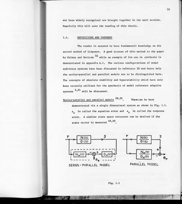
demonstrated in appendix A.l, The various configurations of model

reference systems have been discussed in reference 28 and hence only

the series-parallel and parallel models are to be distinguished here.

The concepts of absolute stability and hyperstability which have only

been recently utilized for the synthesis of model reference adaptive

2 21

systems ' will be discussed.

28 29

Series-parallel and parallel models * . These can be best

demonstrated via a single dimensional system as shown in Fig. 1.1.

e is called the equation error and e is called the response

e t

error, A similar state space structure can be derived if the

. 49,50 state vector is measured

SERIES-PARALLEL MODEL

PARALLEL MODEL

Positive real function 56,58 A rational transfer function G(s)

is termed "positive real" if the following conditions are

satisfied:

(1) G(s) has no poles in Re [s] > 0 and poles on the jw

axis are simple with positive real residues;

(2) Re G(ju) Z 0 for all u>.

It is termed "strictly positive real" if in the above conditions,

the sign > is replaced by z and vice versa.

Positive real matrix ^ . A rational transfer function matrix

Z(s) is termed positive real if:

(1) Z(s) has real elements for real s;

(2) the elements of Z(s) have no poles in Re [s] > 0 and

poles on the jui axis are simple, and such that the

associated residue matrix is non-negative definite Hermitian

(3) Z(joj) + ZT *(ju) 5 0.

The signs T and * denote transpose and complex conjugate

respectively. Similarly a strictly positive real matrix can be

defined.

13 . .

Kalman-Meyer Lemma . This lemma was first stated by Kalman in his

treatment of the Lure problem on absolute stability and was

later modified by Meyer. The result is:

Lemma:

Let A be a real n x n matrix all of whose characteristic

roots have negative real parts, x be a real non­

negative number and b , k be two real n-vectors. If

'V %

x + 2 kT (si - A)“ 1 b

is a positive real function of s then there exist two

12

/ H

d such that

a) A P + P A -d d - Q ;

<\, »V,

rl

b) P b = k + t2 d ;

% r\j 'X*

c) Q is positive semidefinite and P is positive

definite.

For the purpose of using this lemma in the Liapunov

design, one needs to put

t = 0 ;

d

■v 0 so that P b•v

[l, 0 ... 0]

so that k^TjuX - A] 1 b

<\, L J n.

k •V.

k ;

N(joj) D(ju)

where

57

N(s)

D(s) is the transfer function of the plant.

Hypers tability . This term was introduced by V.M. Popov to denote

the stability property of a system consisting of a linear section

and a nonlinear feedback section as shown in Fig. 1.2.

a

Consider the following state space description of the linear

13

x

•\>

y

F x + G u

r\, <\,

H x

(

1

1

where it is assumed that the pair [F, g] is completely

controllable and the pair [f, h] is completely observable.

The vectors u and y are also assumed to have the same <v >v<

dimension.

Kyperstability is a property of the system which requires the

inputs u to satisfy the following inequality: 'Vi

uT ( t ) y ( t ) d t i <$ [ ||x(°) II ] SUP l l x ( t ) II ( 1 . 2 )

Here 6 is a positive constant depending on the initial state

of the system but independent of the time t. The inequality

(1.2) hence defines the allowable class oi nonlinearity.

The system (1.1) is termed "hyperstable" if for any u in the 'Vi

subset defined by (1.2) the folloviing inequality holds for

some positive constant k and for all t:

X ( t ) || i k ( 11x ( ° ) II + 6) (1.3)

The system is termed "asymptotically hyperstable" if for any

u in the subset defined by (1.2) the inequality (1.3) holds

Now lets state the conditions required to^satisfieJby the linear

section of equation (1.1), the transfer function matrix of which

Theorem (Popov) 57: A necessary and sufficient condition for the

transfer function matrix Z(s) of the system (1.1) to define

14

a (asymptotically) hyperstable system is that Z(f) be (strictly)

positive real.

20 • •

Eventual stability . The origin of a system, which solution starts

at time

co and state is said to be eventually stable if,

given e > 0 there exist numbers 6 and T such that

II «0 11 < Ó implies that 11 x ( t , t 0 ,

'V X0> II < e for

all

c * co ? T,

If in addition, there is an r > 0 and a T fl such that

|| x 0 I|<r and tQ i T Q imply.that x (t, tQ , xQ) ^ 0 as

t -*• <» , then the origin is said to be eventually asymptotically

stable.

Theorem (Lasalle and Rath): Consider the following systems (1.4)

and (1.5):

X = F (x, t) 0.4)

X - F (x, t) + P (x,t) 0-5)

<\j r\j %

If the system (1.4) has a uniformly asymptotically stable

origin, then the system (1.5) will be eventually asymptotically

stable if | P. (x. t) | S h (t) when || X II S 13<V0 > °)

J v J 'v

where either:

h. (t) -* o as t -*• “ J

15

CHAPTER 2 - COMPARATIVE STUDIES OF

MODEL REFERENCE ADAPTIVE CONTROL SYSTEMS

2.1. INTRODUCTION

The design of continuous model reference parameter adaptive

control systems has received much attention by the control engineers

in the past fifteen years. Consequently many ingenious design rules

have been reported in the literature. As pointed out in the brief

survey of Section 1.2. there are two main approaches in the synthesis

of this class of M.R.A.C. systems. One is based on the minimization

of a performance index and the other on a Liapunov function

Each of these approaches has its own merits and limitations, although

many modifications have been suggested to improve them further. A

direct contrast of the merits of these designs has been briefly

mentioned in the literature * but a rigorous comparison especially

that from a performance viewpoint has not been reported. Hence a

comparative study of the various design rules will be of great interest

to the designers who have long been faced with the difficulty of

selecting a suitable one for certain applications.

In this chapter attention will initially be focussed on

single-inpui. single-output plant gain adjustment systems. Some of the

more popular rules are critically analysed to point out their relative

merits with regards to the stability, realization and adaptive response,

which will also be supported by some simulation results. Subsequently

a systematic performance comparison based on some well-known criteria

is attempted through simulation studies. Deterministic as well as

stochastic inputs are employed. Sensitivities of the performance to

the input frequency bands are also examined. The interesting and

16

similitudes .

The latter part of this chapter is concerned with the study

of more general parameter adjustments. A qualitative analysis of the

various designs is given and the general concern about noise and

disturbance rejection is also examined.

The design rules to be compared are the M.T.T. rule \ the

2 12 4 . 5

Liapunov synthesis * and the rules suggested by Dressier , Price

13 •

and Monopoli . The first two rules are by now well known while the

latter three are les.' popular. The main reason for choosing the

Dressler's and Price's rules is not merely because of their own merits

but also because they can be viewed as a crude approximation to the

Liapunov design rule with e, replacing the e vector. Hence the effect

of using ej instead of e on the stability and response of the Liapunov

design can be investigated. The inclusion of the Monopoli's rule here

is natural as it is an improved version of the original Liapunov design

with regards to the physical implementation. There are of course other

g . . 25

important design rules such as those due to Kokotovic , Nikiforuk

and Choe . However they are thought to be less general in applications

and possess one or more of the following weaknesses:

(1) time-varying filters are required to generate the

exact sensitivity functions;

(2) at most bounded-input, bounded-output stability can

be ensured;

(3) adaptive gains required to assure convergence are

proportional to the bound on parameter variations -

hence in practice only useful for systems with small

parameter variations;

(4) no integral action in the adaptive loop - hence greater

17

parameter deviations; one such effect is to cause

saturation during the transients;

(5) not truly parameter adaptive - hence not applicable

to system identification problems.

Therefore these latter designs are not included to maintain a feasible

size of the undertaking.

2.2. A CRITICAL COMPARISON OF THE DESIGN RULES

The following analysis is based on the aggregate of knowledge

scattered in the literature. This information is reviewed here and

studied by means of simulations. We shall first compare the M.I.T.

1 2 9-12

rule and the Liapunov synthesis ’ through the design of a g a m

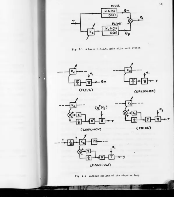
adjustment loop of a linear system as shown in Fig. 2.1. Following

4 . 5

this we shall examine design rules due to Dressier , Price and

13 . . .

Monopoli . The block diagrams of these designs are shown m Fig. 2.2.

2.2.1. M.I.T. Rule and Liapunov Synthesis

The notation used below is that shown in Fig. 2.1 and Fig. 2.2.

The performance index used in the M.I.T. rule ^ is

j

parameter adjustment law using a steepest descent minimization

technique is

K

c Be, !_!3 Ke (2.1)

In this case the sensitivity function

hence the above equation becomes

is proportional to aud

B'e,0

1 m (2.2)

KCD£L

Fig. 2.1 A basic M.R.A.C. gain adjustment system

tM O M O P O Lf)

19

The Liapunov synthesis is based on the use of a Liapunov function

The most successful form of this function V used to date is that

proposed by Gilbart et al . As described in appendix A.I., the

function takes the forms

V = eTPe + X (X + y K m)2

where m = B'e^Pbr

X = K - K K c v

(2.3)

(2.4)

(2.5)

(

2

.

6

)

(2.7) and the time derivative of V is given by

= -e^Qe - 2 Xy K 2 m 2

dt \ v

These result in a stable adjustment law:

K «* m + y m

c

where y is a proportional constant which is chosen to provide

additional damping if required. Putting y = 0 results in the

2

design rule used by Parks .

Equations (2.2) and (2.7) will be compared in the

following manner:

(a) Stability - A stability analysis of equation (2.2) is very

difficult. The doubt about possible instability has been demonstrated

o ,

by Parks for a second order system with step inputs. Even for a

23

first order system with a sinusoidal input, James has obtained a

complicated stability domain in the parameter space. This domain is

shown here in Fig. 2.3(a) to demonstrate the complications «-hat arise.

Further studies by James ^ have revealed the stability problems

associated with stochastic inputs and the lack of adequate theoretical

methods to predict the stability boundary. An example is shown here

in Fig. 2.3(b). Hence extensive simulations during the design stage

Fig. 2.3 Stability regions of M.I.T. DESIGNS

/ , t 23,24.

21

hand equation (2.7) is assured to be stable Tor all inputs such that

e 0 asymptotically, with the assumption that K is slowly time-

% v

varying. When this assumption is severely violated, a stability

problem similar to that of equation (2.2) may arise. 'Eventual

stability', however, can be assured by using a theorem due to Lasalle

and Rath (see Section 1.4) if the time-varying function belongs

20

to the following class :

|Kv (t)| s n(t) (2.8)

where n(t) 0 as t -*• "

or n(t) dt is finite.

^0

(b) Physical Realization - Equation (2.2) can be easily implemented

and it is this distinct advantage that has made M.R.A.C. a popular

adaptive control strategy. Equation (2.7) however, requires the

estimation of the complete state vector which is not often available

and hence necessitates the use of differentiating networks which cause

a noise amplification problem, or the use of adaptive state observers

17 18

' which further complicate the implementation.

(c) Response - The speed of adaptation of both equations depends

on the magnitudes of the adaptive gain B' and the input signal R. A

large B' is always necessary to maintain a high speed of adaptation.

However as B' and R vary, the damping of the response will also vary.

11

12

Root locus plots of these equations for a second order system '

2

would show that when B'R is large, the M.I.T. design will be under­

damped while the Liapunov design will be adequately damped with suitable

values of the proportional gain y .

2.2.2. Other Design Rules

We shall next examine the following rules.

4

hand equation (2.7) is assured to be stable for all inputs such that

e -»■ 0 asymptotically, with the assumption that K is slowly time-

% v

varying. When this assumption is severely violated, a stability

problem similar to that of equation (2.2) may arise. 'Eventual

stability', however, can be assured by using a theorem due to Lasalle

and Rath (see Section 1.4) if the time-varying function belongs

20

to the following class :

21

where

|Kv (t)| $ n(t)

n(t) + 0 as t -*■ "

l(t) dt is finite.

(

2

8

r-<

(b) Physical Realization - Equation (2.2) can be easily implemented

and it is this distinct advantage that has made M.R.A.C. a popular

adaptive control strategy. Equation (2.7) however, requires the

estimation of the complete state vector which is not often available

and hence necessitates the use of differentiating networks which cause

a noise amplification problem, or the use of adaptive state observers

17 18

’ which further complicate the implementation.

(c) Response - The speed of adaptation of both equations depends

on the magnitudes of the adaptive gain B' and the input signal R. A

large B' is always necessary to maintain a high speed of adaptation.

However as B' and R vary, the damping of the response will also vary.

11 12

Root locus plots of these equations for a second order system ’

2

would show that when B'R is large, the M.I.T. design will be under­

damped while the Liapunov design will be adequately damped with suitable

values of the proportional gain y.

va

fc

22

K = B'e,r (2.9)

c l

The resulting controller is very simple and no sensitivity filter is

required. The disadvantages are that the damping of the response suffers

at larger loop gains and that the global stability is not guaranteed.

Its stability problem is similar to that of the M.I.T. rule.

Price ^ ---- The parameter adjustment law which is called the accel­

erated gradient method is

K = B 'e ir + y c It (B'e ir) (2-10)

where v is a constant. ' c

The controller is similar to that of Dressier except for the

addition of the proportional (feedforward) term. This term has the

effect of improving the damping and the stability of the response.

This stabilising effect would however be impaired as the order of the

system increases, and generally the global stability cannot be guaranteed.

13

Monopolr --- This is based on a modification of the Liapunov

scheme. A differentiating block (Z(s)) is used to modify the plant

transfer function such that Z(s)N(s)/D(s) is positive real, and the

Kalman-Meyer Lemma (see Section 1.4) is used to eliminate the error

derivatives required in equation (2.7). Hence

K c = B'eiy + y (B'eiy) (2.11)

where y is the modified input signal to the plant and obtained by

passing the original signal through a filter (1/Z(s)). For an n-th

order plant with m zeros, the order of Z(s) is (n-m-1). Global

asymptotic stability of the adaptive loop will be guaranteed while the

number of derivatives required is reduced to (n-m-1), or

(n-m-2) if the extra damping loop is not in use. The latter is achieved

by decomposing Z(s) into Z'(s)(s + a). Now since K is available,

23

This technique can be easily extended to the case of a general time-

varying gain.

2.2.3. A Simulation Study of the Adaptive Response

At this point one would wonder whether or not the stability

issue should have an important weight at all on assessing a design

rule. For instance if the M.I.T. design, subject to a stability

analysis or simulation which defines the domain of stable operations,

would in this stable domain exhibit a faster speed of adaptation than

the Liapunov design, then the former would be regarded as practically

adequate and the emphasis on achieving global stability should be

lessened. If the reverse is true then the requirement for the design

to guarantee global stability will be more acceptable and useful to

the system designers. Such an issue, which has so far been neglected

in the literature, will be investigated here.

various designs has been conducted. The adaptive response is defined

in this context as the time response of the parameter adjustment when

there is a step change in the parameter. The study has indeed shown

that very often the Liapunov designs could achieve excellent performance

not attainable by other rules. As an example consider a second order

plant whose gain is to be adjusted. Referring to Fig. 2.1 and 2.2, the

following values are assumed:

A simple simulation study of the adaptive response of the

N(s) 1

a i *> 2 , a 2 ■= 1 , K “ 1 ,

D(s)

l+a1s+a2s2

25

Z(s) = 2s + 2 (as in Ref. 13) and shall limit the values of y and

to, say, 50% because in actual use they may have to be quite small

to reduce the effect of any noise at the plant output and the excessive

transient overshoots due to large initial errors. Some of the typical

adaptive responses of the various designs are depicted : • Fig. 2.4

for step as well as sinusoidal inputs. The responses shown for the

M.I.T., Dressier and Price designs have been optimized with respect

to the convergence time. The responses shown for the Liapunov and

Monopoli's schemes are, however, not optimized - i.e. they can still

be further improved if required by increasing the adaptive gain. From

this simulation study, the M.I.T. design is found to be unstable for

B' > 1. Even when it is stable at lower values of B ' , the response is

slow, the convergence time being well over five system time constants.

The response of the Dressier scheme to a step input is similar to that

of the M.I.T. scheme. However, for a sinusoidal input, the Dressier

scheme shows a steady state parameter error which is dependent on the

loop gain as well as the input signal frequency. The design due to

Price shows a better damping and stability which improve as y c is

increased. On the other hand, the Liapunov design is always stable

and the damping and convergence can be improved systematically by

varying B' and y. A convergence time of even less than one system

time constant can be easily achieved. The design due to Mor.opoli,

which does not require any differentiator in this case, exhibits quite

a fast response. Although its damping would suffer at higher B', the

system stability would always be maintained. These results also

substantiate the foregoing theoretical analysis.

2.3. A SYSTEMATIC PERFORMANCE COMPARISON

The importance of a performance comparison has been discussed

V

26

in Section 2.2.3. The example given also indicates the complexity and

scale involved in any attempt to make a complete comparative study.

A systematic approach is therefore taken in this section.

30

Some commonly used performance criteria which include the

settling time (Tg) , the integral of squared error (ISE) , the integral

of time absolute error (ITAE), and the integral of time squared error

(ITSE) will be employed to compare the responses of the various designs

against their system parameters. This will be studied experimentally

through computer simulations of two gain adjustment schemes. The

results will be presented in the form of similitudes by applying a

31

dimensional analysis to the system differential equations such that

the quantities to be investigated are expressed in dimensionless

groups. The dimensionless performance criterion is denoted by m,

a n d a;m er\V tonl«ss s y s te m pam m eH n is ¿«.»voted b y *6». .

The performance characteristics are defined in this connection as the

plots of TTj against m2>

, N(s) 1 \

2.3.1. First Order Systems ( --^ -y = "J+sT '

In this case, the designs due to Dressier and Price are

identical to the Liapunov schemes. Also, the latter does not require

any differentiators. Hence we only need to compare the M.I.T. and

the Liapunov designs. Their system equations are listed in appendix

A .2.

Deterministic inputs --- Step and sinusoidal inputs are employed.

From the dimensional analysis shown in appendix A.3. the following

are defined:

m„ = KK B'R2T (M.I.T. design)

2 V

27

= T /T

s (5% Tg criterion)

KRT2 K 2R2T 1 1

; iei2dt

(ITAE criterion)

K2R2T 2 1

(ITSE criterion)

The parameters which cannot be grouped into the above are fixed at:

frequency of sinusoidal input = 2.5 c/s, Kc (tQ) - 0, y = 0 and

0

.

1

.

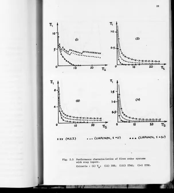
2.5 and 2.6. For step inputs, in which case the M.I.T. design is

always stable, the Tg criterion shows a region where this design is

unfavourable since Xj may increase or decrease with an increment in

tt2 , whereas the same type of uncertainty does not appear in the

Liapunov design with y = 0.1. For sinusoidal inputs, all the four

characteristics for the M.I.T. design possess regions of uncertainty

over a wide range of ir2< Furthermore it has already been ensured

that within the parameter ranges tested, that is it s 25, this

design is operated below the boundary of conditional stability as

pointed out by James (Fig. 2.3 (a)). These findings suggest that an

extensive simulation study would be necessary in order to determine

a safe and economic value of tt2 t0 achieve any specific tTj even

though the system is operated in the stable region. On the other hand,

the similitudes for the Liapunov designs show a monotonic decrease of

tt1 with increasing ir2 . This is a desirable feature. In addition this

design can achieve values of ttj not attainable by the M.I.T. design.

Examinations of the effect of changing the input signal frequency have

also been conducted. The results which are too long to show here,

indicate that in the M.I.T. scheme the system performance is very

28

X X X (M .I.T.)

. . . (UAPC?NOV, < “ O )

( L

, t » 0 .0

Fig. 2.5 Performance characteristics of first order systems

with step inputs.

it is almost insensitive to the frequency especially at higher gains.

Stochastic inputs --- The above experiment is repeated with a

band-limited Gaussian white noise input. This stochastic signal is obtained

by spacing a digitally generated, zero mean, Gaussianly distributed

sequence of pseudo random numbers, by an interval of h seconds and

with linear interpolations. The variance of the signal is denoted by

and its power spectrum which is approximately flat possesses a

cutoff frequency of l/2h Hz . The properties and generation of

this stochastic signal are further discussed in appendix A.4. To

reduce the complexity of this investigation, only the ISE criterion

will be studied in detail.

where e[ ] denotes the expectation (i.e. ensemble average) operator.

The fixed parameters are: h = 0.002, K ^ t g ) = 0.0, y = 0 or 0.1.

similitudes show that both the M.I.T. and Liapunov designs exhibit the

desirable characteristics that iij decreases monotonicaiiy with

increasing The latter also achieves a much lower tr^ which

cannot be reached by the former. Another important property that has

been noted is that the variances about the expected values are different

in each case. From the plot shown in Fig. 2.7(b), one observes that the

variances in the M.I.T. design are very much larger than those in the

Liapunov scheme. This indicates that in the former scheme there may

exist a considerable degree of uncertainty about its performance. This The dimensionless quantities are:

IT

2 = KK B'6.2 v N t (M.I.T. design)

= K B'6.2 T

v N (Liapunov design)

31

X X X ( M . X . T . ) . . . ( U R P U N O V , % — O ) A A A ¿URPUNOV, * = 0 -l)

Fig. 2.7 Performance characteristics of first order systems

with stochastic inputs.

¿1

XXX ('M.I.T.') . . .

c

Fig. 2.8 A sample of the characteristics

33

is confirmed by studying the ensemble members of the random process.

One of these is shown here in Fig. 2.8. Also shown are ensembles of

the corresponding results using the other two integral criteria. These

similitudes reveal that the M.I.T. scheme possesses the undesirable

that in the Liapunov scheme shows an almost monotonic decrease.

In addition to the case just reported, other experiments

have been carried out. The finding is that when the power spectrum

of the input signal (proportional to l/h) is reduced, the performance

of the M.I.T. design would deteriorate whereas that of the Liapunov

design would improve.

here. The system differential equations are as listed in appendix A.2.

It is noted that while the Liapunov design requires one differentiator,

that due to Monopoli does not need any.

Deterministic inputs ---- From the dimensional analysis shown in

appendix A.3. the following are defined:

property that ir may increase or decrease with increaiing ir2 while

2.3.2. Second Order Systems ( d(s)" ”

1+a s+a s2

1 2

1

)

The five designs described in Section 2.2. will be examined

TT 2

■= KK B'R2a,

v 1 (M.I.T. design)

- K B'R2a,

v 1 (others)

(2% T criterion) s

1

Cj 2dt (ISE criterion)

K 2R 2a 1

— — tlejdt

KR a 2

= --- -— te 2dt (XTSE criterion)

K 2R2a2 J 1

Other fixed parameters are: a2/a2 = Kc (tQ) = Yc =

Y = 0 and 0.1, frequency of sinusoidal input = 0.16 c/s.

The performance characteristics obtained are shown in Fig.

2.9 and 2.10. With step inputs, the M.I.T. and Dressier designs

possess a minimum in it as tt2 varies; for tt2 smaller or larger

than this minimum value, it increases sharply. Other designs show

a monotonic reduction, especially at higher values of tt2> With sine

inputs, both the M.I.T. and Dressier designs are again found to possess

a minimum in iTj, and the latter is more critical than the former.

The design by Price shows an unfavourable performance in that the

uncertainty as discussed in the first order systems occurs. The

Liapunov and the Monopoli designs, however, still maintain the

desirable performance characteristics similar to that with step inputs.

The performance of these designs with different frequencies

of the sinusoidal input signal has also been examined. The same range

of tt2 is used. The general observation is that the Liapunov and

Monopoli designs are less sensitive to the signal frequency with

regards to both the stability and the convergence rate. The M.I.T.

system always possesses a minimum iTj at some value of tt2 which

increases with the frequency; at lower frequencies, more than one

minimum point may be observed. The convergence rate decreases with

increasing frequencies. The Dressier system is unstable at higher

frequencies; at lower frequencies the system is stable for a small

range of it but this range may increase or decrease with decreasing

frequencies. The design by Price improves at lower frequencies, in

that the fluctuation in ir reduces, but deteriorates rapidly at

frequencies higher than the resonant frequency of the plant and

35

*xx ( M J . - O . . . (LIBPUNOV,

%

%

coo CMONOPOU') d o b ¿ P R IC E , O .5 } T , f ('D R E S S L E R ')

< _ > OR |

C

Fig. 2.9 Performance characteristics of second order systems

with step inputs.

X X X (M.I.T.)

(LIR P o N O V , Ti = 0 )

( HRPuMOV, X = o -O

OOO (MONOPOLl) B O B

(

P R IC E ,

= 0 -5 )

r T T

C

D R E S S L E R )

t > oR ^ ( C H A N G E IN S C A L I N G )

Big. 2.10 Performance characteristics of second order systems with sinusoidal inputs.

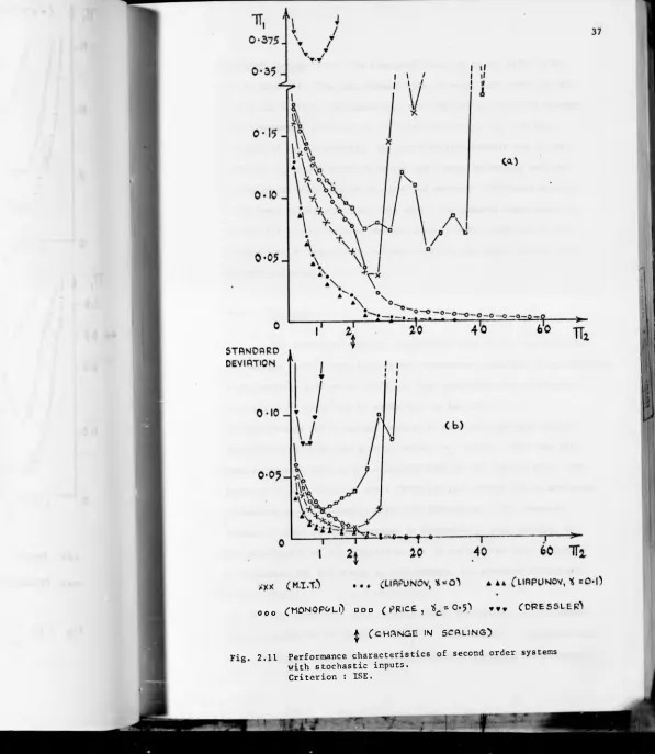
o o o CMONOP&Ui) O D D ( P R I C E , 1<c = 0 * 5 ) T t f ( D F E S S L E R )

^ C C H A N G E IN S C A L I N G )

Fig. 2.11 Performance characteristics of second order systems with stochastic inputs.

Stochastic inputs --- The same experiment as in the first order

case is repeated. The main results with h = 0.1 are shown in Fig.

2.11(a) and 2.11(b). To summarise, the Liapunov and Monopoli designs

exhibit monotonic decrease of it with increasing ir2 and the

variances of Hj are small; the other designs exhibit one or more

minima in it and the variauces are also large indicating serious

uncertainty as mentioned in the previous section. Different spectra

of the input signal have also been used. The general observation is

that the M.I.T. <-nd Dressier designs exhibit worse performance when

the bandwidth of the signal is reduced, while the other designs show

improved performance.

2.3.3. Summary

The extensive computer simulation study of the various M.R.

A„C. designs reveals many interesting properties regarding the performance

of the adaptive systems at different loop gains and under different

input signals. These may be summarised as follows:

(1) The designs which are not assured to be stable globally behave

very differently when the gain parameter it varies. They are also

found to be sensitive to the frequency band of the input signal; one

reason of this is that the total effective gain varies due to different

attenuation by the system at different frequencies. The possible

outcome of these two disadvantages is instability, poor damping, or

poor convergence of the adaptation. It is unfortunate that in trying

to compensate for the change in environment, the adaptive system may

become sensitive to its own parameters.

(?) The performance of those designs which are assured to be globally

stable improves as the gain parameter it increases. In addition they

39

content by operating at larger values of n2>

(3) Among the three schemes based on gradient methods, the Dressier

design exhibits the worst performance characteristics especially when

the input is sinusoidal or stochastic. The M.l.T. design is quite

acceptable if the performance specification is not very strict. The

design by Price performs better than the M.l.T. system with step or

stochastic inputs but is inferior with sinusoidal inputs.

(4) The two designs based on stability consideration may achieve low

values of tTj not attainable by other designs. Between the two,

the Liapunov scheme is better as it requires s lower value of ir

to meet the same performance criterion. On interchanging the roles of

the model and the plant, the case studied would become an identification

system. Hence this investigation also reveals the shortcomings of those

37 38

model reference identification schemes ’ based on gradient methods.

2.4. GENERAL DISCUSSIONS

In the previous sections, no attempt has been taken to

include the study of more general parameter adjustments and the effects

of noise and disturbance inputs. Hence an examination of these

general concerns is in order and presented herewith.

b ^ and a ^ respectively. The parameter adjustment laws using the

M.I.T. rule, the Dressier rule and the Liapunov synthesis are shown

in Table 2.1. For simplicity the proportional term in the Liapunov

design is put to zero; the laws due to Price and Monopoli are also

not included as they are extensions of the Dressier and Liapunov designs

and hence trivial for the purpose of comparing structures.

40

Rules M.I.T. Dressier Liapunov

b . =

Pi gi * e i * rif

(i) Bi ' e l • r

T (i)

Bi * < * % > ■ r

a . =

Pi "“i • el • °if

-a. • e . ( P

i 1 m

X (i)

-°i ' ■ ep

Table 2.1.

The ^ denotes the ith differentiation with respect to time and r.f

and 0., are defined as if

41

economical compared to the M.I.T. rule since both require r and

(i)

0 to be accessible. While the e can be readily generated using

C t ^ ( i ) ^

O and 0 , each r., and 0.„ would require one additional

p m if if M

filter having the same order as that of the model.

The Liapunov design has been synthesized to assure global

asymptotic stability while the M.I.T. and Dressier designs could only

be proved to be locally stable. It is observed that the stabilizing

factor in the Liapunov design is due to the presence of a . In this

s.

aspect, the other designs which use e^ only would seem to be less

stable as the system crder increases.

In short the M.I.T. rule is found most undesirable; the

Dressier rule offers the advantage of simplicity while the Liapunov

synthesis guarantees global asymptotic stability. It is sufficient

here to mention that the reduction of the order of differentiation,

the introduction of proportional damping and the treatment of time-

varying parameters can easily be incorporated in the Liapunov design.

(i)

2.4.2. Effects of Noise

We shall analyse the effect of including the process and

sensor noise in the plant output. 0^ is assumed to be the only

measurable output while r, r ^ and 0^ are assumed noise free. Thus

0 . 0., and e will have noise components. As is well known

P P if

in the case of parameter estimation system, the presence of noise

components may introduce d.c. bias in the steady state values of the

a . parameter and hence contribute to additional e.rror to the plant

output. To investigate this possibility, we shall make use of the following

equation.

a = a • e • 0 (2.15)

Let e„, 0„ and a be the respective noise free values, e and

o * o o n