A Block Preconditioned Inexact Linear Solver for Computing the Complex Eigenpairs of a Large Sparse Matrix

(1)

http://www.scirp.org/journal/jamp ISSN Online: 2327-4379

ISSN Print: 2327-4352

DOI: 10.4236/jamp.2018.62040 Feb. 28, 2018 429 Journal of Applied Mathematics and Physics

A Block-Preconditioned Inexact Linear Solver

for Computing the Complex Eigenpairs of a

Large Sparse Matrix

Richard Olatokunbo Akinola

1*

, Stephen Yakubu Kutchin

1

, Ayodeji Sunday Ayodele

1

,

Kingsley Obiajulu Muka

2

1_{Department of Mathematics, Faculty of Natural Sciences, University of Jos, Jos, Nigeria} 2_{Department of Mathematics, University of Benin, Benin, Nigeria}

Abstract

In computing eigenpairs of the matrix pencil, one obtains a linear system of equations. In this work, we show how a block triadiagonal preconditioner in GMRES can be used to solve a large sparse unsymmetric system of equations inexactly using a fixed and decreasing tolerance. While the fixed tolerance solver converged superlinearly to the eigenvalue of interest, the decreasing one converged quadratically. This surpasses an earlier result which converged harmonically.

Keywords

Preconditioner, Superlinear Convergence, Quadratic Convergence, Eigenvalues

1. Introduction

Let

A

be a large sparse, real n by n nonsymmetric matrix and _B_∈n n× a

symmetric positive definite matrix. In this paper, we consider the problem of computing the eigenpair

( )

z,λ from the following generalized complex eigen-

value problem

, n, ,

λ

= ∈ ≠

Az Bz z  z 0 (1)

where λ∈__{is the eigenvalue of the pencil}

(

A B,

)

and z its corresponding

complex eigenvector. We assume that the eigenpair of interest

( )

z,λ is alge-

braically simple, with ψH_{the corresponding left eigenvector such that}_[1]

0.

H _≠

Bz

ψ ₍₂₎

How to cite this paper: Akinola, R.O., Kutchin, S.Y., Ayodele, A.S. and Muka, K.O. (2018) A Block-Preconditioned In-exact Linear Solver for Computing the Complex Eigenpairs of a Large Sparse Ma-trix. Journal of Applied Mathematics and Physics, 6, 429-445.

https://doi.org/10.4236/jamp.2018.62040

Received: December 21, 2017 Accepted: February 25, 2018 Published: February 28, 2018

http://creativecommons.org/licenses/by/4.0/

(2)

DOI: 10.4236/jamp.2018.62040 430 Journal of Applied Mathematics and Physics

By adding the normalization

1,

H ₌

z Bz (3)

to (1), the combined system of equations can be expressed in the form

( )

=

F z 0 as

( )

(

₁

)

₁ .

2 2

H λ

 − 

 

=_ _=

− +

 

 

A B z

F z

z Bz 0 (4)

Note that H

z Bz is real since B is symmetric and positive definite. This

results in solving a system of nonlinear n complex and one real equation for the

1

n+ complex unknowns v=

[ ]

z,

λ

T. The reason we cannot use Newton’s

method to solve (4) is because z in the normalization z BzH =z BzT is not

differentiable.

Recall that for a real eigenpair

( )

z,λ , (4) is

(

n+1

)

real equations for

(

n+1

)

real unknowns and Newton’s method for solving (4) involves the

solution of the

(

n+1

)

square linear systems

( ) ( )

( )

( ) ( )

( )

(

)

( )

( )T ( )

T ₁ ₁ ,

0

2 2

k k

k

k k k k

λ λ

λ

 ₋ 

 ₋ ₋ __∆ _ _ _

 _ __{= −}_ _

₋ ___∆ __ _₋ ₊ _

  _ _

A B z

A B Bz _z

Bz _z _Bz (5)

for the

(

n+1

)

real unknowns ∆v( )k = ∆_ z( )kT,∆λ( )k _, and updating

(k+1)₌ ( )k _{+ ∆} ( )k

v v v . Secondly, if instead of the normalization (3), we add

1

H =

c z , where c is a fixed complex vector (see, for example, [2]), (1) and 1

H ₌

c z provide

(

n+1

)

complex equations for

(

n+1

)

complex unknowns,

and the Jacobian of this new system is

(

)

. 0 H

λ

− −

 

 

 

A B Bz

c

The above Jacobian is square and can be easily shown to be nonsingular, using the ABCD Lemma [3] if the eigenvalue of interest is algebraically simple and

0

H ≠

c z . Thirdly, if

( )

z,λ is complex, then, as stated earlier, we have n

complex and one real equation. Also, if z solves (4), then so does eiθ

z for any θ, such that 0≤ ≤ πθ 2 .

Our approach for analyzing the solution of (4) for v begins by splitting the

eigenpair

( )

z,λ into their real and imaginary parts: z= +z₁ iz₂, λ α= +iβ

where 1, 2

n ∈

z z  , and α β, ∈. After expanding (4), we will obtain a real 2n+1 under-determined system of nonlinear equations in 2n+2 real un-

knowns

[

]

T

1, 2, ,

α β

=

v z z , and it is natural to use the Gauss-Newton method

(3)

DOI: 10.4236/jamp.2018.62040 431 Journal of Applied Mathematics and Physics Algorithm 1. Computing the complex eigenvalues of the pencil

(

A B,

)

.

Input: A B J, , , ( )0 ( )0 ( )0 T ( )0 ( )0 1 , 2 ,α β,

 

=  

w z z , kmax,

1) for k=0,1, 2, until convergence do

2) Solve Mu=B w1 for u:

 _{Find the lu factorization of} M i.e., [L U, ]=lu( )M .

 _{Solve the lower triangular system} Lc=B w1 for c.

 Solve the Upper triangular system Uu=c for u.

3) Compute T

1

α=

n w B Ju and T

1

β=

n w B u

4) Form the matrix

.

β α

α β

−

 

=  

 

n n

T

n n

5) Find the LU factorization of T, that is [L U, ]=lu( )T

6) Solve

(

)

(

)

T 1 T

2 1

1 2

1

L

 ₊ 

 

=  

 ₊ 

 

 

w

w B w

c _{n w}

u

for c.

7) Solve Uω=c for α β ∆   =  _∆  

ω .

8) Form the vector +_{= ∆}α _{− ∆}β

w u Ju.

9) Update

.

α α

α

β β

β

+

∆     ₌ ₊      _∆       

10) end for

Output: (max) (max) (max) (max)

, ,

k  k αk βk 

=  

v w .

The main mathematical tools used in this paper are the LU factorization, inexact inverse iteration and preconditioned Generalized Minimal Residual (GMRES) [9]. The main reason for using inexact inverse iteration is due to the fact that as mentioned in an earlier paper, we do not solve Mu=B w1 , in

practice but we will use it to show that the solution is possible. Theorem 2.1 shows that the Jacobian has a single nullvector at the root, while Theorem 3.1 gives an important orthogonality result. Algorithms 1-3 are presented. We remark that in the limit, the approximate nullvector converges to the exact. A numerical example is given which supports the validity of the algorithms presented though, as usual, relies on good initial guesses to the desired eigenpair. The classical inverse iteration for the matrix pencil converges slowly for some eigenvalue problems while we present algorithms that converge quadratically. Throughout this paper, unless otherwise stated all norms are the 2-norm.

The following result helps to enforce the validity of the results in this paper. Lemma 1.1: [10] Let Fw

( )

w be of full rank. If Fw

( )

w ∆ =w F w

( )

, is an

under-determined linear system of equations, then its least squares solution

( )

( ) ( )

1

( )

T T−

∆ = −w Fw w _Fw w Fw w _ F w , is orthogonal to the nullspace of

( )

w

(4)

DOI: 10.4236/jamp.2018.62040 432 Journal of Applied Mathematics and Physics Algorithm 2. Inexact inverse iteration algorithm.

Input: A B, , ( )0 ( )0 ( )0 ( )0 ( )0 T 1 , 2 ,α β, ,kmax

 

=  

w z z .

for k=0,1, 2,, until convergence

Choose τ( )k

. Solve ( ) ( ) ( )

1

k k ₌ k

M u B w inexactly,

( ) ( ) ( ) ( )

1 1

1 .

k k k _τk

− ₋ − _≤

M u B w

 

end for Output: _u(kmax).

Algorithm 3. Complex eigenvalues of the pencil

(

A B,

)

using Inexact Inverse Iteration with preconditioning.

Input: A B J, , , ( )0 ( )0 ( )0 ( )0 ( )0 1 ; 2 ,α β,

 

=  

w z z , kmax, tol

for k=0,1, 2, until convergence do

Solve ( ) ( ) ( ) 1

k k ₌ k

M u B w inexactly using Algorithm 2.

Compute T

1

α=

n w B Ju and T

1

β=

n w B u

Solve

(

T

)

1 1

1

, for . 2

0

β α

α β

α α

β β

 

− ∆ ∆

  ₌_ + _  

  _∆  _ _ _∆ 

   

  __ __

n n w B w

n n

Form the vector +_{= ∆}α _{− ∆}β

w u Ju.

Update

.

α α

α

β β

β

+

∆     ₌ ₊      _{  }_∆ _  

end for

Output: (kmax)=  (kmax)_,α(kmax)_,β(kmax)



v w .

In the next section, we will express both z and λ as λ α= +iβ and 1 i 2

= +

z z z , convert the nonlinear system (4) to a real under-determined system

of nonlinear equations and prove some important results.

2. Computation of Complex Eigenpairs by Solving an

Under-Determined System of Nonlinear Equations

In this section, we will expand the system of nonlinear n complex and one real equations in n+1 complex unknowns (4) by writing z and λ as

1 i 2

= +

z z z and λ α= +iβ , respectively. The reason for having an under-

determined system of equations instead of a square system of equations is because, expanding H =1

z Bz gives only one real equation, since B is sym-

metric positive definite, while

(

A−λB z

)

=0 results in 2n real equations. This

results in a 2n+1 real under-determined system of nonlinear equations in 2n+2 real unknowns. This will then be followed by presenting the under-

determined system of nonlinear equations and explicit expression for its Jacobian. Furthermore, we will show in the main result of this section-Theorem 2.1 that if the eigenvalue of interest in

(

A B,

)

is algebraically simple, then the

(5)

Jacobian at the root and proof that it is unique.

If we let z= +z1 iz2 and λ α= +iβ, then the square nonlinear system of

Equations (4) can be written as

(

)

(

) (

)

(

)

(

)

1 2

1 2 2 1 ,

i i

i

λ α β

α β α β

− =_ − + _ +

= − + + _ − − _

A B z A B z z

A B z Bz A B z Bz (6)

and

T T

1 1 2 2.

H = +

z Bz z Bz z Bz (7)

Hence,

(

T T

)

1 1 2 2

1 1 1 1

.

2 2 2 2

H

− z Bz+ = − z Bz +z Bz + =0

Since

(

A−λB z

)

=0, we equate the real and imaginary parts of (6) to zero

and obtain the 2n real equations

(

A−αB z

)

1+βBz2=0 and

(

A−αB z

)

2−βBz1=0. This means, F v

( )

consists of the 2n real equations

arising from (6) and one real equation

(

T T

)

1 1 2 2

1 1

0

2 2

− z Bz +z Bz + = ;

( )

(

)

(

)

1 2

T T

1 1 2 2

,

1 1

2 2

α β

β α

 

 ₋ ₊ 

 

=_ − + − _=

 

− + +

 

 

A B z Bz

F v Bz A B z

z Bz z Bz

0 (8)

where (2 2) (2 1)

: n+ → n+

F   . The Jacobian F vv

( )

of F v

( )

which has the

following explicit expression

( )

(

)

(

)

( )

(

)

1 2

2 1

T T

1 2

,

0 0

α β

β α

 ₋ ₋ 

 

= − − − − 

 

− −

 

 

v

A B B Bz Bz

F v B A B Bz Bz

Bz Bz

(9)

is a 2n+1 by 2n+2 real matrix. From the Jacobian (9) above, we define the

real 2n by 2n matrix M as

(

)

(

)

.

α β

β α

 − 

=  ₋ ₋ 

 

A B B

M

B A B (10)

Also, we form the 2n by 2 real matrix

[

]

1 2

1 1 1

2 1

,

−

 

=_ _= − − −

 

Bz Bz

N B w B w

Bz Bz (11)

consisting of the product of 1

  =    

B O

B

O B and the matrix of right nullvectors

of M at the root, where

1 2

1

2 1

, ,

    =_{ } =_ _

−    

z z

w w

z z (12)

and O is the n by n zero matrix. The Jacobian (9) can be rewritten in the

(6)

( )

(

)

(

)

1 1 1

T T T

1 1 , 0 0 −     =  =  − −         v

M B w B w M N

F v

B w B w 0 (13)

with M, N are as defined in (10) and (11) respectively. Note that because at

the root,

(

)

(

)

12

(

)

12 21

,

α β α β

β α α β

 −    − + 

= =

 ₋ ₋    ₋ ₋   

   

A B B z A B z Bz

B A B z A B z Bz 0

this implies that 1 2

     

z

z or its nonzero scalar multiple is a right nullvector of M.

In the same vein, we find

(

)

(

)

21

{

(

)

21 12

}

, α β α β α β β α − −    −    =_ _=  ₋ ₋  ₋  ₋ ₋ ₊        

A B z Bz

A B B z

A B z Bz

B A B z 0

and 2 1

  ₋   

z

z or its nonzero scalar multiple is also a right nullvector of M at the

root. Since the eigenvalue λ_of

(

A B,

)

is algebraically simple by assumption,

then by (2), we need to give explicit expressions for the left nullvector of

(

A−λB

)

in order to prove that the Jacobian has full row rank at the root.

Observe that if we define ψ ψ= 1+iψ2 , where 1, 2 \

{ }

n

∈_ 0

ψ ψ for all

(

λ

) { }

H\

∈ A− B 0

ψ

_{, then this implies}

(

)

(

)

(

)

(

)

(

)

T T 1 2

T T T T T

1 2 1 2 .

H

i i

i

λ α β

α β β α

− = − _ − − _

 

= − − − _ + − _=

A B A B B

A B B B A B 0

ψ ψ ψ

ψ ψ ψ ψ

Hence, T

(

)

T T

1 A−αB −β 2B=0

ψ ψ and T T

(

)

T

1 2

βψ B+ψ A−αB =0 . The

implication of this is that

(

)

(

)

(

)

(

)

T T T T

1 2 1 2

T T T T

1 2 1 2 .

T

α β

β α

α β β α

 −    = _ _     ₋ ₋     =_ − − + − _=

A B B

M

B A B

A B B B A B 0

ψ ψ ψ ψ

which means, T T 1, 2

 



ψ ψ

 or its nonzero scalar multiple is a left nullvector of M. Similarly,

(

)

(

)

(

)

{

(

)

}

T T T T

2 1 2 1

T T T T T

1 2 1 2 ,

α β

β α

β α α β

 −   −  = − _ _     ₋ ₋     =_ + − − − − _=

A B B

M

B A B

B A B A B B 0

ψ ψ ψ ψ

and it shows that T T 2, 1

 − 



ψ

 is also a left nullvector of M.

So we form the matrix C consisting of the 2-dimensional left nullvectors of M at the root (in practice C is not computed), as

1 2 2 1 .   =  ₋   

C ψ ψ

ψ ψ (14)

Now, observe that the condition (2), implies

T T T T

1 1 2 2 1 2 2 1 0.

H

i

   

=_ + _+ _ − _≠

Bz Bz Bz Bz Bz

(7)

Therefore, at the root, either T T 1Bz1+ 2Bz2≠0

ψ ψ or T T

1Bz2− 2Bz1=0

ψ ψ ;

T T

1Bz1+ 2Bz2 =0

ψ ψ _or T T

1Bz2− 2Bz1≠0

ψ ψ _{or both} T T

1Bz1+ 2Bz2

ψ ψ _and

T T

1Bz2− 2Bz1

ψ ψ are nonzero. It excludes the possibility that they are both zero. Before we continue with the rest of the analysis, we pause a little to present the main result of this section which shows that the Jacobian (9) has a one dimensional nullvector at the root.

Theorem 2.1 Assume that the eigenpairs

( )

z,λ of the pencil

(

A B,

)

are

algebraically simple. If z1 and z2 are nonzero vectors, then T T

2, 1, 0, 0

τ

 

= _z −z _

φ

_,τ∈ is the unique nonzero nullvector of F vv

( )

at the

root.

Proof: See [5].

After linearizing F v

( )

=0, we have the following under-determined linear

system of equations

( )

k _∆ ( )k _{= −}

( )

( )k _. v

F v v F v (15)

Let ( )k

n be the exact nullvector of the Jacobian F v_v

( )

( )k . By adding the

extra condition T ( )

0 k

∆ =

n v , which stems from Lemma 1.1 to the under-

determined linear system of Equations (15), we obtain the following square linear system of equations

( )

T .

0

k _k

k

   

 _∆ _{= −}_ _

  _ _

 

v

F v F v

v n

(16)

3. Square System of Equations for the Numerical

Computation of the Complex Eigenvalues of a Matrix

In the preceding section, we saw that by adding an extra equation to the under-determined linear system of equations 15, we obtained a square system of equations (16). However, in practice we would never compute ( )k

n , but

Theorem 2.1 guarantees the existence of a unique nullvector _φ( )k _{at the root.}

This is the motivation for the discussion in this section. In this section, we will use φ( )k _{defined by} ( ) ( ) ( )

2 , 1 , 0, 0

k ₌ k ₋ k 

z z 

φ as an approximation to n in (16)

and show that the solution obtained by solving (15) is equivalent to the solution obtained by solving

( )

T ,

0

k _k

k

   

 _∆ _{= −}_ _

  _ _

 

v

F v F v

v

φ (17)

in the absence of round off errors. To do this, we will show that ( )T ( ) 0 k _∆ k ₌

v φ

for each k, and this is presented in the main result of this section: Theorem 3.1. Algorithm 1 is given for computing an algebraically simple eigenpair of the pencil

(

A B,

)

. Note that since M has been shown to be singular at the root in

section 2, this section is anchored on the assumption that when v is not at the

root, M is nonsingular.

(8)

DOI: 10.4236/jamp.2018.62040 436 Journal of Applied Mathematics and Physics 0

, 0

  = ₋   

I J

I (18)

and

1 2

2 1

0

. 0

     

=_ __{  }= _ − −

     

z z

I Jw

z z

I (19)

The matrix J satisfies the following properties:

1) T_{= −}

J J.

2) T 2n =

J J I , where I2n is the 2n by 2n identity matrix.

3) 2 2n. = −

J I

4) The matrix J commutes with M, i.e., JM=MJ.

5) For _∈ 2n

w  , w B JwT 1 =w JB wT 1 =0.

6) Let u be an unknown vector that solves Mu=B w₁ . By premultiplying

both sides by J we obtain JMu=JB w₁ and hence MJu=JB w1 because of

the commutativity of M and J. Therefore, if Mu=B w₁ , then Ju solves

( )

= 1

M Ju JB w.

We begin by writing the linear system of Equations (15) explicitly. For ease of notation, we shall drop the superscripts and define +_{= + ∆}

w w w where (k+1)

+₌

w w , and replace w( )k and _∆z₁( )k T,∆z₂( )kT_ with w and ∆w respec-

tively. This means that (15) can now be rewritten as:

(

)

1 1

T T

1 1

,

1 1

0 0

2 2

α β ∆

   

−

 _{  } _ _

∆ = −

 _{  } _ _

− +

−

 

 _{  }__∆ _ __ __

w _Mw

M B w B Jw

w B w

B w (20)

which is equivalent to the following system of equations

1 1

α β

∆ − ∆ + ∆ = −

M w B w B Jw Mw

T T

1 1

.

2 2

−w B w∆ = w B w−

After rearrangement, the first n-equation reduces to

1 1 .

α β

+_{− ∆} _{+ ∆} ₌

Mw B w B Jw 0 (21)

By multiplying both sides of the

(

n+1

)

th equation by 2, we obtain:

T T

1 1

2w B w∆ +w B w=1.

This in turn reduces to

(

)

T

1 + ∆2 =1.

w B w w (22)

Observe that since +_{= + ∆}

w w w, 2∆ =w 2w+−2w and

2 2 +

+ ∆ = −

w w w w. Now,

(

)

(

)

T T T T

1 2 1 2 2 1 1

+ +

+ ∆ = − = −

w B w w w B w w w B w w B w. Consequently,

(

)

T T

1 1

1

1 . 2

+₌ ₊

w B w w B w (23)

(9)

(

)

(

)

1 1 T T 1 1 . 1 1 0 0 2 α β +  _{ } _ −  _{   } _ ∆ =  _{   } _ +     _∆  _   w

M B w B Jw

w B w B w

0

(24)

We assume that the 2n by 2n matrix M is nonsingular except at the root.

This is what forms the basis for the following discussion. That is to say, we want to show that when not at the root, ( )T ( )

0 k _∆ k ₌

v

φ .

First of all, let the exact nullvector n of

( )

(

)

1 1 T 1 , 0 0 −   =   −     v

M B w B Jw

F v

B w

be defined as T

, α, β

 

=  w 

n n n n , where _∈ 2n

w

n  , n n_α, _β are real scalars, Jw

and M are defined respectively by (19) and (10). Hence,

(

)

1 1 T

1

,

0 0 α

β   −  _{  } =  _{  } −      _{ } w n

M B w B Jw

n B w

n 0

then after expanding the matrix-vector multiplication, we obtain

(

)

1 1

α β

− + =

w

Mn n B w n B Jw 0 (25)

T

1 w=0.

w B n (26)

We make distinctly clear at this juncture, that the nullvector T

, _α, _β

 

=  w 

n n n n

is not exactly the same as

( )

T

, 0, 0

 

=  Jw 

φ because, the later has the form of the exact nullvector at the root, but is evaluated at the kth iterate while the former is the nullvector even when not at the root.

Another way of writing (24) is as follows

1 1 .

α β

+_{= ∆} _{− ∆}

Mw B w B Jw (27)

This means that we could solve (24) by solving

1 ,

=

Mu B w (28)

for u. After which the solution of (27) is given by .

α β

+_{= ∆} _{− ∆}

w u Ju (29)

With this expression for +

w , it can be observed that

1

1 1 1 1 .

α β α β

+_{= ∆} _{− ∆} _{= ∆} _{− ∆}

= ∆ − ∆ = ∆ − ∆

Mw Mu MJu B w JMu

B w JB w B w B Jw

Which means that +

w is well defined. Furthermore, from (25)

(

)

1 1 ,

α β

= −

w

Mn n B w n B Jw

using the fact that J commutes with B1 and (28) gives

.

α β

= −

w

n n u n Ju (30)

Since w is B₁-orthogonal to nw by virtue of Equation (26), taking the B1-

inner product of both sides of the above with w yields

T T T

1 w= α 1 − β 1 =0.

(10)

From which we deduce

T T

1 and 1 .

α= β =

n w B Ju n w B u (31)

Consider the problem of solving the under-determined linear system of Equations (20) for the 2n+2 real unknowns ∆ = ∆v _ wT,∆ ∆

α β

, _. It was

stated in Lemma 1.1 that the minimum norm solution to an under-determined linear system of equations is orthogonal to the nullspace. It is an application of this result that yields the following important relationship:

T T

0=n ∆ =v n_w∆ + ∆ + ∆w n_α α n_β β. (32)

If we add the nullvector n to the last row of (24), then

(

)

(

)

1 1

T T

1 1

T

1

0 0 1 .

2 T

α β

+  

−

   _{ } _

   _{ } _

∆ = +

   _{ } _

  __∆ _ _ _

 w  _ _

w

M B w B Jw _w

B w w B w

n n n

n w

0

(33)

By expanding the second to the last row, T

(

T

)

1 1

1

1 2

+₌ ₊

w B w w B w . But from

(29), + _{= ∆}α _{− ∆}β

w u Ju. This implies that, by taking the inner product of both

sides with w, yields

(

)

(

) (

)

T T T T

1 1 1 1

1

1 . 2

α β

+_{= ∆} _{− ∆} ₌ ₊

w B w w B u w B Ju w B w

Using the definition (31) for nα and nβ, we obtain

(

T

)

1

1 , 2

β∆ − ∆ =α α β +

n n w B w (34)

where the unknown quantities ∆α and ∆β are to be determined, so we need an extra equation to be able to do so. The last row of the matrix-vector multiplication (cf. (33)) above comes from (32) since

(

)

(

)

T

T T T

0

.

α β

+

= + ∆ + ∆

= + ∆ + ∆ + ∆

= + ∆ + ∆ + ∆ =

w

w w w

n w n n

n w w n n

n w n w n n n w

If we substitute the expression (30) for nw and (29) for

+

w into the left hand

side, then one obtains

( )

T

[

]

T T _.

α β α β α α β β

 ₋  _∆ _{− ∆} _{+ ∆ + ∆ =} n u n Ju  u Ju n n n ww

Furthermore, by expanding the first term on the left hand side, using the properties of J, then

( ) (

T

)

T

T T T

2 2

.

α β

 ₋  _∆ _{− ∆}

 

= ∆ + ∆

n u n Ju u Ju

n u u n u J Ju

n u n u

(11)

(

)

(

)

2 2

2 T

1 .

α β α β

α β

α β α β

α β

∆ + ∆ + ∆ + ∆

= + ∆ + ∆ = _w

n u n u n n

u n n n w

Observe that because u is real,

(

1+ u 2

)

is nonzero. Accordingly, after

dividing both sides by

(

2

)

1+ u

(

)

T

2 .

1 α∆ + ∆ =α β β

+

w n w

n n

u (35)

We combine the two equations (34) and (35) below

(

)

(

)

T 1 T 2 1 1 2 , 1 β α α β α β  ₊    − ∆    _{ } _ =   _∆ _{ } _     _ _ +     w w B w

n n

n w

n n

u

(36)

to compute ∆α_and ∆β simultaneously. The matrix on the left hand side is always nonsingular except at the root (in which case all entries are zero), this is because, its determinant is 2 2

α+ β

n n . Equation (35) can now be applied to

simplify

(

)

(

)

(

)

(

)

T T 1 1 T 1 T T 1 1 0. α β α β α β α β α β +₌ _∆ _{− ∆} = ∆ + ∆ = ∆ + ∆ = ∆ + ∆ =

w B Jw w B J u Ju

w B Ju u

w B Ju w B u

n n

(37)

Notice that we have used the property 2 2n = −

J I to arrive at the second step

above and the definition (29) for +

w .

Next, we want to establish the orthogonality of φ and ∆v in the next key

result. Before we do that, notice from Theorem (2.1) that φ, at the root, is a scalar multiple of T T

2, 1, 0, 0

 − 

z z  and by the definition of J in (18), we can

also write

( )

T

, 0, 0

 

=  Jw 

φ _{, with} T T

1, 2

 

=  

w z z . This result holds when v=v( )k

is at the root or not, but because the analysis used to establish the orthogonality is based on the assumption that M is nonsinsingular when not at the root. As a

result of this, after presenting Algorithm (1) (to follow shortly), we then show that the same result holds when M is singular at the root.

Theorem 3.1 Let φ be an approximation to the exact nullvector n of

( )

v

F v . Then, φ is orthogonal to ∆v.

Proof: To proof this, recall that T

, ,

α β

 

=  

v w , v+= w+T,α β+, +_ and

( )

T

, 0, 0

 

=  Jw 

φ _{. This implies}

(

)

( )

T

(

)

T T T T T T

T T T

0,

+ + +

+ +

∆ = − = − = − = − = − =

v v v Jw w w w J w w J w

w Jw w Jw w Jw

φ φ

(38)

showing that T

0

∆ =v

φ _{. In arriving at the last step above, we have used the}

properties of J and a special case of (37) where B₁=I₂_n.

(12)

The first is the 2n by 2n linear system of equations in (28), while the second is the 2 by 2 linear system (36).

Stop Algorithm 1 as soon as

( )k _, tol

∆v ≤

where ∆ =v _w+−w,

ω

_. The above analysis shows that T

0

∆ =v

φ _when ( )k v

is not at the root. Next, we want to show that the same result holds at the root. In a manner analogous to the proof of Lemma (2.1), we postmultiply both sides of the above system of equation by T

C where C is the 2n by 2 real

matrix defined by (14), consisting of the left nullvectors of M. If M and N

are as defined respectively in (10) and (11), then, this is the same as

T T

. α β

+₊ ∆ ₌

_∆   

C Mw C N 0

But by the definition of C, the first term on the left hand side of the equation

above is zero, since T ₌ T

C M 0 . It can be recalled from the proof of Lemma 2.1

that the 2 by 2 real matrix ₌ T

H C N is nonsingular at the root. This implies

(

T T

)

T T

1 1 2 2 1 2 2 1

T

T T T T

1 2 2 1 1 1 2 2

.

α α α

β β β

₋ ₊ ₋ 

∆ ∆ ∆

     

= =  =

_∆  _∆  _∆ 

 

    _ − + _ 

Bz Bz Bz Bz

C N H

Bz Bz Bz Bz

0

ψ ψ ψ ψ

Accordingly, ∆ = ∆ =α β 0 because of the nonsingularity of H. Therefore,

.

+₌

Mw 0 (39)

From the property of M at the root, it has two nonzero nullvectors and

hence singular. The implication of this fact and the above is that, +

w is in the

nullspace of M. But, we have already established that the nullspace of M

consists of T T T 1, 2

 

=  

w z z and w₁=Jw=_z₂T,−z₁T_. Hence, we can write

1.

µ τ

+₌ ₊

w w w

Now, from the last equation in (24),

(

)

(

)

T T T T

1 1 1 1 1

T T T T

1 1 2 2 1 1

1

1 2

.

µ τ

µ τ µ

+

+ = = +

= + − =

w B w w B w w B w w B w

w B w z Bz z Bz w B w

Consequently,

T 1 T

1

1 . 2

µ=w B w+

w B w

But at the root, T T T 1 = 1 1+ 2 2=1

w B w z Bz z Bz . Therefore, µ=1, w+=w,

1 1 +₌

z z and 2 2 +₌

z z . This will now be used to deduce the following corollary at

the root.

Corollary 3.1 Let

( )

T

, 0, 0

  =  Jw 

φ . Let T

,α β,

+ _ + + +_

=  

v w . Then, φ is orthogonal to ∆v at the root.

Proof: This follows from the second to the last line of the proof of Theorem 3.1 (cf., Equation (38)) where +₌

(13)

T T T

0.

+

∆ = −v w Jw = −w Jw= φ

4. Inexact Inverse Iteration with Preconditioning

for Solving (28)

In Section 2, we found two nonzero nullvectors for M at the root. As a result

of this property of M at the root, in this section, we will describe an inexact

inverse iteration technique for solving the large sparse system of Equations (28) in step 2 of Algorithm 1 and present Algorithm 2 and Algorithm 3. Result of a numerical experiment is given which supports the theory in Section 5.

We give the following version of inexact inverse iteration in Algorithm 2. We will use a fixed tolerance. Note that because of the special nature of M at the

root, the choice of a preconditioner is crucial for convergence to the desired accuracy to be achieved. The inexact linear solver that we use is the preconditioned GMRES [9] where we define the following block tridiagonal preconditioner,

.

α β

α

−

 

≈  ₋ 

 

A B B

A B

 (40)

Next, we present Algorithm 3, which is the inexact inverse iteration equi- valence of Algorithm 1. The stopping criterion for the outer iteration in

Algorithm 3 depends on the norm of the eigenvalue residuals, that is

( )

(

( )

)

( ) ( ) ( )

1 1 2 ,

k k k k k

tol

α β

= − + ≤

r A z Bz

and

( )

(

( )

)

( ) ( ) ( )

2 2 1 ,

k k k k k

tol

α β

= − − ≤

r A z Bz

and

and .

tol tol

α

β +

∆

  _≤ ₋ _≤ _∆ 

  w w

5. Numerical Experiments

As mentioned earlier, the sparse linear system of equations in step 2 of

Algorithm 1 is solved with an LU type factorization of M which is expensive

and besides the L and U factors may have more nonzero elements than M. In

this section, our main goal is to use preconditioned GMRES with the block triangular preconditioner  in (40) to solve the system Mu=B w1 inexactly.

We do this by considering a single numerical experiment with a fixed and a decreasing tolerance. Results are presented by means of tables and figures.

Example 5.1

Consider the 200 by 200 matrix A bwm200.mtx from the matrix market

library [12]. It is the discretised Jacobian of the Brusselator wave model for a chemical reaction. The resulting eigenvalue problem with B=I was also

(14)

which is closest to the imaginary axis and its corresponding eigenvector. In this example, we take ( )0 ( )0

0.0, 2.5

α = β = _{in line with}_[13]_{and took}

( )0 1 = 2

z 1 1 and z2( )0 =1 1 , where 1 is the vector of all ones.

In Table 1 and Table 2, we present results for the computation of the eigenpairs

( )

z,λ for the matrix in Example 5.1, and stop once the norms of

[

]

T

,

α β

∆ ∆ _{and the eigenvalue residuals} ( ) 1

k

r and r₂( )k are smaller than the

outer tolerance 14

outer 2.5 10

τ ₌ _× − _._f_{represents the number of inner iterations}

[image:14.595.201.538.369.735.2]

used by preconditioned GMRES to satisfy the fixed inner tolerance τ=0.6 in Table 1, while d in Table 2 represents number of inner iterations used by preconditioned GMRES to satisfy the decreasing inner tolerance

( )

{

}

inner min 0.6, 0.6 1

k

τ = r . Quadratic convergence to 1.81999e 05 2.13950i

λ= − + _{is easily observed from the second up to the}

seventh iterates in columns five and six of Table 2. However, this quadratic convergence is lost in the last iterate. This could be due to the fact that we are solving a nearly singular system as we approach the root. As shown in columns five and six of Table 1, as we approach the root, more number of inner iterations

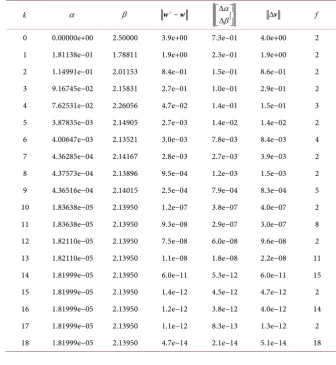
Table 1. Table showing convergence to the eigenvalue λ=1.81999e−05+2.13950i with a fixed inner tolerance for Example 5.1. The last column shows the number of inner iterations it took to satisfy the fixed inner tolerance τ=0.6.

k α β w+−w α

β ∆   _∆ 

  ∆v f

0 0.00000e+00 2.50000 3.9e+00 7.3e−01 4.0e+00 2

1 1.81138e−01 1.78811 1.9e+00 2.3e−01 1.9e+00 2

2 1.14991e−01 2.01153 8.4e−01 1.5e−01 8.6e−01 2

3 9.16745e−02 2.15831 2.7e−01 1.0e−01 2.9e−01 2

4 7.62531e−02 2.26056 4.7e−02 1.4e−01 1.5e−01 3

5 3.87835e−03 2.14905 2.7e−03 1.4e−02 1.4e−02 2

6 4.00647e−03 2.13521 3.0e−03 7.8e−03 8.4e−03 4

7 4.36285e−04 2.14167 2.8e−03 2.7e−03 3.9e−03 2

8 4.37573e−04 2.13896 9.5e−04 1.2e−03 1.5e−03 2

9 4.36516e−04 2.14015 2.5e−04 7.9e−04 8.3e−04 5

10 1.83638e−05 2.13950 1.2e−07 3.8e−07 4.0e−07 2

11 1.83638e−05 2.13950 9.3e−08 2.9e−07 3.0e−07 8

12 1.82110e−05 2.13950 7.5e−08 6.0e−08 9.6e−08 2

13 1.82110e−05 2.13950 1.1e−08 1.8e−08 2.2e−08 11

14 1.81999e−05 2.13950 6.0e−11 5.3e−12 6.0e−11 15

15 1.81999e−05 2.13950 1.4e−12 4.5e−12 4.7e−12 2

16 1.81999e−05 2.13950 1.2e−12 3.8e−12 4.0e−12 14

17 1.81999e−05 2.13950 1.1e−12 8.3e−13 1.3e−12 2

(15)

[image:15.595.204.539.135.586.2]

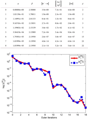
DOI: 10.4236/jamp.2018.62040 443 Journal of Applied Mathematics and Physics Table 2. Table showing quadratic convergence to the eigenvalue

1.81999e 05 2.13950i

λ= − + _{with a decreasing tolerance for Example 5.1. The last}

column shows the number of inner iterations it took to satisfy the decreasing inner tolerance min 0.6, 0.6

{

1( )

}

k

τ = r .

k α β w+−w α

β ∆   _∆ 

  ∆v d

0 0.00000e+00 2.50000 3.9e+00 7.3e−01 4.0e+00 2

1 1.81138e−01 1.78811 1.9e+00 2.3e−01 1.9e+00 2

2 1.14991e−01 2.01153 8.4e−01 1.5e−01 8.6e−01 2

3 9.16745e−02 2.15831 2.7e−01 8.0e−02 2.8e−01 3

4 1.19965e−02 2.15159 3.8e−02 1.7e−02 4.1e−02 5

5 3.56419e−04 2.13989 7.2e−04 5.4e−04 9.0e−04 7

6 1.79381e−05 2.13950 2.6e−07 3.8e−07 4.6e−07 13

7 1.81999e−05 2.13950 4.0e−14 4.5e−14 6.0e−14 22

8 1.81999e−05 2.13950 2.1e−14 5.2e−14 5.6e−14 22

Figure 1. Convergence history of the eigenvalue residuals on Example 5.1 with a fixed tolerance τinner =0.6.

were needed to satisfy the decreasing inner tolerance as against the fixed tolerance. From Table 1, we observed superlinear convergence in columns five and six.

(16)

[image:16.595.211.534.77.323.2]

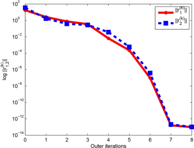
DOI: 10.4236/jamp.2018.62040 444 Journal of Applied Mathematics and Physics Figure 2. Convergence history of the eigenvalue residuals on Example 5.1 with a decreasing tolerance inner min 0.6, 0.6

{

1( )

}

k

τ = r .

superlinearly in Figure 1, we observed a quadratic decrease in the norm of the eigenvalue residuals in Figure 2. It is quite surprising to see that Algorithm 3

works because M is singular at the root, which means we solved a singular

system at the root.

6. Conclusions

While Ruhe ([2] Section 3) used the normalisation H ₌1

c z and solved the

resulting

(

n+1

)

by

(

n+1

)

nonlinear system of equations to obtain

[ ]

z,

λ

T.

We have been able to show that, with the addition of the non differentiable normalisation z zH =1, it is still possible to convert the resulting system of

under-determined nonlinear equations into a square one.

Nevertheless, in this work, we obtained Algorithm 1 which consists of a combination of a 2n -by-2n system of equations (which is the same as those in

[13]) and a 2-by-2 system. A numerical example show that using an LU-solver on the one hand and preconditioned GMRES as an inexact solver on the other hand to solve the large sparse 2n-by-2n system of Equations (28), followed by the 2 by 2 system in each case, give similar results in the limit. By and large, the algorithms presented in this paper relies on good initial guesses to the desired eigenpair of interest.

Acknowledgements

(17)

References

[1] Stewart, G.W. (2001) Matrix Algorithms. Vol. II, Eigensystems, SIAM.

[2] Ruhe, A. (1973) Algorithms for the Nonlinear Eigenvalue Problem. SIAM Journal on Matrix Analysis and Applications, 10, 674-689. https://doi.org/10.1137/0710059 [3] Keller, H.B. (1977) Numerical Solution of Bifurcation and Nonlinear Eigenvalue Problems. In: Rabinowitz, P., Ed., Applications of Bifurcation Theory, Academic Press, New York, 359-384.

[4] Deuflhard, P. (2004) Newton Methods for Nonlinear Problems. Springer, 174-175. [5] Akinola, R.O. (2014) Theoretical Expression for the Nullvector of the Jacobian:

In-verse Iteration with a Complex Shift. International Journal of Innovation in Science and Mathematics, 2, 367-371.

[6] Akinola, R.O. and Spence, A. (2014) Two-Norm Normalization for the Matrix Pen-cil: Inverse Iteration with a Complex Shift. International Journal of Innovation in Science and Mathematics, 2, 435-439.

[7] Akinola, R.O. and Spence, A. (2015) Numerical Computation of the Complex Ei-genvalues of a Matrix by solving a Square System of Equations. Journal of Natural Sciences Research, 5, 144-157.

[8] Akinola, R.O. (2015) Computing the Complex Eigenpair of a Large Sparse Matrix in Complex Arithmetic. International Journal of Pure & Engineering Mathematics

(IJPEM), 3, 137-158.

[9] Saad, Y. and Schultz, M.H. (1986) GMRES: A Generalized Minimal Residual Algo-rithm for Solving Nonsymmetric Linear Systems. SIAM Journal on Scientific and Statistical Computing, 7, 856-869. https://doi.org/10.1137/0907058

[10] Boyd, S. (2008/2009) Lecture 8: Least Norm Solutions of Under-Determined Equa-tions, EE263 Autumn.

[11] Freitag, M.A. and Spence, A. (2009) The Calculation of the Distance to Instability by the Computation of a Jordan Block, Linear and Nonlinear Eigen Problems for PDEs, 274-275.

[12] Biosvert, B., Pozo, R., Remington, K., Miller, B. and Lipman, R. Matrix Market. http://math.nist.gov/MatrixMarket/