Nonlinear methods for inverse problems

(1)

A thesis

presented for the degree of Doctor of Philosophy

in Mathematics

from the University of Canterbury, Christchurch, New Zealand

T. John (})nnolly B.Sc. (Hans), M.Sc.

(2)

(3)

equation. The solution of this via the Newton-Kantorovich method is outlined. Frechet differentiability of the operator is given by the implicit function theorem. We also consider questions such as uniqueness, stability and regularization of the inverse problem.

This general theory is then applied to a number of different inverse problems. The Newton-Kantorovich method is derived for each example and Fnkhet differentiability examined. In some cases numerical results are provided, for others our work provides a theoretical basis for results obtained by different authors.

(4)

(5)

ACKNOWLEDGEMENTS

I would like to express my sincerest thanks to Dr D.J.N. Wall, for his assistance and supervision over the years taken for this research.

I would also like to thank Dr RJ. Astley, Civil Engineering Department and Professor R.H.T. Bates, R. Murch and Dr D.G.H. Tan, all from the Electrical and Electronic Engineering Department, for useful discussions and their encouragement. In addition, I thank Mrs B. Bristowe for her typing of this thesis.

(6)

(7)

PREFACE

Inverse or identification problems often takes the form of determining an unknown function, which is a coefficient in a partial differential equation. Another type of inverse problem commonly encountered, in inverse scattering for example, is where the unknown quantity is a boundary of the region on which the problem is defined.

The inverse problem is distinct from the direct or forward problem, where the coefficient function or boundary of the problem is known. Then we have the partial differential equation to solve, subject to boundary conditions, if there are any.

To be able to solve the inverse problem, extra information is required in the form of measurements of the solution of the corresponding direct problem. Some inverse problems are linear in nature, often requiring the solution of an integral equation of the first kind. However, for many inverse problems, there is a nonlinear relationship between the measurements and the solution of the problem.

(8)

Problems such as the existence, uniqueness and characterization of solutions of the inverse problem are also outlined. In addition we consider properties of the resulting operator-such as continuity, Frechet differentiability and compactness. The instability resulting from the compactness of the operator requires the use of regularization methods. The examination of such questions is necessary before a numerical implementation of our methods is attempted.

In Chapter Two the properties of the direct problem for the steady-state diffusion equation are examined. Existence, uniqueness and regularity results are given for both classical and weak solutions of the equation.

In Chapter Three an inverse problem from steady-state diffusion, with interior measurements, is investigated. Direct identification and the stability of the inverse problem are first reviewed. Newton methods are then derived for the solution of this inverse problem. Frechet differentiability and compactness are shown for the nonlinear operator utilized and the application of regularization techniques outlined. In the chapter numerical results from the solution of a one-dimensional problem are given - these incorporate regularization methods in the presence of measurement noise.

In Chapter Four inverse problems for boundary scattering are considered. We utilize the implicit function theorem to obtain the continuous dependence of the farfield upon the boundary. Expressions for the Frechet derivative of this map are derived via the null field method and also variational methods. Finally we investigate the determination of an unknown impedance boundary condition from farfield measurements and a Frechet differentiability result is proven for this problem.

(9)

integral equation formulation are also considered. Numerical solutions of the equation are discussed.

In Chapter Six we consider the determination of a spatially var)'lng refractive index in the Helmholtz equation. This inverse problem is formulated as a non linear operator equation and the Newton-Kantorovich method for its solution derived. Frechet differentiability is proven for both continuous refractive indices and square integrable indices for which the Born series converges. The Frechet derivative is shown to be compact with point measurements and regularization methods examined.

Chapter Seven investigates an inverse problem from geometric optics. Newton's method and regularization techniques are outlined for the inverse problem and these are related to work of other authors.

In Chapter Eight a summary and conclusions are presented, and also some suggestions for future research relating to the work in this thesis.

During the course of my studies the following papers and report were prepared:

1. T.J. Connolly, D.J.N. Wall and R.H.T. Bates. Inverse Problems and the Newton-Kantorovich fl.1ethod. In AJ. Devaney and R.H.T. Bates, editors, "Inverse Optics II", pages 30-34, Proceedings SPIE volume 558, August 1985.

2. T.J. Connolly and D.J.N. WalL An Inverse Problem, with Boundary 111easurements fo1' the Steady State Diffusion Equation, Research Report 40, Department of Mathematics, University of Canterbury, Christchurch, New Zealand, October 1987.

(10)

4. T.J. Connolly and D.J.N. Wall. On Frechet Differentiability of Non-Linea1\ Operators occurring in Inverse Problems - an Implicit Function Theorem,

Approach, to be submitted to "Inverse Problems".

The third paper forms the appendix of this thesis.

(11)

!RN !R n

lxl

sup in£

n

an

supp u

n9'

CUcn)

NOTATION

product of n copies of the real line !R dual of !Rn

1 . n

= (xr

+ ... +

x~) 2 , the euclidean norm on !R

supremum, or least upper bound, of a set of real numbers infimum, or greatest lower bound, of a set of real numbers bounded domain in !Rn

closure of

n

= f!\f! 'boundary of

n

the support of u (smallest closed set outside which u = 0) Multiindex Notation

-product of n copies of the set Z

+

of non-negative integers

n

=

a1

+ ... +

an , where the n-tuple 9' f Z

+

a a

= ( fJ / &.1) 1 .. . ( fJ / fJxn) n , ( 9' E Z

~

)

Main Function Spaces

space of real continuous functions on the closure

n

(supposed to be compact) of

n,

equipped with the maximum norm

space of real functions, defined and m times continuously differentiable in f! (m E Z

+

Or ill =

+

00)

(12)

subspace of

Bm(n)

consisting of the functions all of whose derivatives of order ~ m can be extended as continuous functions to the closure

n

of

n '

equipped with the norm

l!ull

= max sup

I

Dau(x)

I

0~

I

al ~m ~en

-subspace of C00(fl) consisting of the functions having compact support; elements of C~(fl) are often referred to as test functions inn

subspace of Cm(fl) consisting of those functions u for which, for 0 ~

I

al < m , Dau satisfies a Holder condition of exponent A, equipped with the norm

llullm, \

= max sup

/

O~lal~m~,ycn

I!:f-Y

I

Dau(J!:)·Dau(y)

I

~~-

y

I

Lebesgue space of measurable functions u such that the pth power of the absolute value

I

u I is integrable over

n

(1 ~ p <

+

oo) , equipped with the norm

I

PI~=

[f

lu(x)IPdx] l/p

n

Lebesgue space of measurable functions u in

n

which are essentially bounded, equipped with the norm

lpl!

00, the essential supremum of

(13)

Hm(D) H~(D) H-m(fl)

H\K)

Sobolev space of functions u in D such that D0'u t: LP(D) for all n-tuples 0' e: Z +,

I

a!

~ m (D0' denotes distribution derivative)

;::::; wm•2(D) , a Hilbert space closure in Hm(D) of C~ (D)

space of distributions u in fl which can be written as finite sums of derivatives of order ~m of functions belonging to L2(fl) (me: Z+) the Sobolev space of order s e: IR in IRn , i.e. the space of tempered distributions u in IRn whose Fourier transform

u

is a measurable function such that

+oo

(14)

(15)

1.5 THEORETICAL CONSIDERATIONS 24

1.5.1 Review 25

1.5.2 Frechet Differentiability 27

1.5.3 The Implicit Function Theorem 30

1.5.4 Lipschitz Continuity 33

1.5.5 Compactness 34

1.5.6 Summary 37

2. STEADY-STATE DIFFUSION EQUATION 41

2.1 INTRODUCTION 41

2.2 ClASSICAL SOLUTIONS 43

2.2.1 Integral Representations 45

2.2.2 Existence and Uniqueness

(16)

3.

AN lNTERIOR MEASUREMENT PROBLEM

51

3.1

INTRODUCfiON

51

3.1.1

Direct Identification

52

3.2

ITERATIVE METHODS

55

3.2.1

Newton-Kantorovich Method

56

3.2.2

Gauss-Newton Method

62

3.2.3

Equivalence of Methods

65

3.3

ONE-DIMENSIONAL PROBLEM

67

3.3.1

An Example

68

3.3.2

An Integral Equation

70

3.4

NUMERICAL IMPLEMENTATION

72

3.4.1

S.V.D. Regularization

73

3.4.2

Numerical Results

74

3.5

THEORETICAL CONSIDERATIONS

82

3.5.1

Frechet Differentiability

82

3.5.2

Lipschitz Continuity

86

3.5.3

Compactness

88

3.5.4

Regularization

89

3.6

BOUNDARY MEASUREMENTS

92

3.6.1

Additional References

93

4.

INVERSE BOUNDARY SCATIERING

95

4.1

INTRODUCfiON

95

4.2

THE INVERSE PROBLEM

97

4.2.1

Uniqueness

98

4.2.2

Continuous Dependence

98

4.2.3

Construction of Solutions

101

4.2.4

Vector Problems

104

4.3

IMPUCIT FUNCTION THEOREM

104

4.3.1

Boundary Integral Equation

104

4.3.2

107

4.3.3

The Frechet Derivative

110

4.4

NULL FIELD METHOD

114

4.4.1

Direct Problem Solution

115

(17)

4.5

THE FRECHET DERIVATIVE

120

4.5.1

Variational Approach

120

4.5.2

Hadamard Variation

124

4.5.3

A Linear Problem

126

4.6

IMPEDANCE PROBLEM

127

4.6.1

128

4.6.2

Generalized Solutions

133

4.6.3

The Fn§chet Derivative

134

5.

THE MODIFIED HEIMHOL1Z EQUATION

135

5.1

INTRODUCTION

135

5.1.1

An Integral Representation

136

5.1.2

Existence and Uniqueness

137

5.2

AN INTEGRAL EQUATION

140

5.2.1

Weakly Singular Integral Operators

141

5.2.2

Regularity

143

5.3

BORN SERIES

146

5.3.1

Regularity

148

5.4

SOVOLEV SPACE THEORY

152

5.4.1

Uniqueness

155

5.4.2

Existence and Regularity

157

5.5

NUMERICAL SOLUTIONS

161

6.

INVERSE REFRACTIVE INDEX SCATTERING

163

6.1

INTRODUCTION

163

6.1.1

Uniqueness

164

6.1.2

Preview

165

6.2

NONLINEAR OPERATOR APPROACH

166

6.2.1

166

6.2.2

Alternative Schemes

168

6.2.3

Phase Problems

173

6.3

THEORETICAL CONSIDERATIONS

175

6.3.1

175

6.3.2

Born Series Result

180

6.3.3

Lipschitz Continuity

184

6.3.4

Compactness

187

(18)

6.4

FAR-FIELD MEASUREMENTS

191

6.4.1

192

6.4.2

Born Approximation

194

6.4.3

197

6.4.4

Completeness and Uniqueness

201

6.5

STEEPEST DESCENT

203

6.5.1

Inverse Problem Application

204

6.6

RICCATI WAVE EQUATION

205

6.6.1

Rytov Approximation

206

6.7

CHAPTER ONE

THE GENERAL INVERSE PROBLEM

1.1 INTRODUCTION

A problem of much interest in physics and engineering is the determination of the interior properties of an object. To enable this, the object is probed with some incident field (for example electromagnetic or acoustic waves). Measurements of the resulting field are then performed either on the object's surface or exterior to it. From these measurements the relevant interior properties are to be deduced. Often the location and shape of such an object must also be determined from farfield measurements. Problems of this form arise in geophysical prospecting, nondestructive testing, remote sensing, medical imaging and related areas.

A mathematical description of the problem is the determination of a spatially-varying coefficient function in a region. This function is generally a coefficient in a partial differential equation. Knowledge of the solution of this equation is used to determine the coefficient function.

The conventional solution of the partial differential equation (p.d.e.) is known as the direct problem. That of determining the coefficient function is known as the inverse or identification problem. A selection of review papers on inverse problems is Boerner et al. [1981], Parker [1977a], Polis and Goodson [1976], Sabatier [1983] and Sleeman [1982].

(20)

applied to solving particular problems in later chapters.

1.2 TilE GENERAL PROBlEM

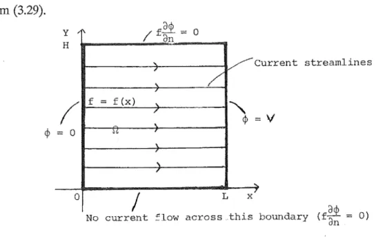
We denote by v(~) the spatially varying function to be determined on a region

n,

such as in Figure 1.1. This function is a coefficient in a partial differential equation (or perhaps an integral equation). The solution of this] equation is denoted by y(~).

M

Figure 1.1

The problem will be considered in a function space setting. The coefficient function, v, is required to belong to a subset,

Xo,

of a Banach space X.

(21)

the direct problem is a nth order partial differential equation then Y is a space of n times continuously differentiable functions (typically cfl(n)).

We shall assume the functions v and y are related by an operator equation of the form

ecv,y) = 0 . (1.1)

Here

e :

Xo

® Y --+ W, where W is another Banach space. This equation incorporates possible initial/boundary conditions on y -

e

then maps into a product space resulting from the differential equation and the additional conditions.

The partial differential equation in question is generally defined on either of two types of regions. Firstly, it is defined on a compact region such as

n

in Figure 1.1, then the measurements of the direct problem solution are made on the boundary

an.

Alternatively, the equation may be defined on an unbounded region containing

n -

such as IRn. This situation occurs often in wave propagation problems. Then measurements are made on a surface, M, exterior to

n

and the coefficient function, v, is known outside

n.

We do however consider one problem where the measurements may be performed in the interior of

n.

Such problems though are generally easier to solve than the corresponding boundary or exterior measurement problems.

Inverse problems resulting from several different direct problems shall be tackled in this thesis.

(i) An example that will be considered in much more detail in later chapters is the following elliptic p.d.e. (with Dirichlet boundary conditions), occurring in steady-state heat and electric current flow :

v.

(f(~)V ¢(Y:;)) ¢(~)- g(r:)

o,

x

c- n

(22)

Here the function to be reconstructed, f, corresponds to v in (1.1), and the solution of the direct problem ¢ corresponds to y. An alternative boundary condition for this problem is the Neumann condition

Here -//.;denotes the normal derivative to the boundary.

(ii) Another problem considered in this thesis is for the modified Helmholtz, equation

where '¢ is the field and a spatially-varying refractive index, n, is to be reconstructed. Closely related to this is the Schrodinger equation

where '¢ is the probability density function and V the potential. Both these equations arise in wave propagation problems and are subject to a condition at infinity known as the radiation condition. The determination of a scattering boundary in the Helmholtz equation proper (i.e. with n

=

1) is also examined.

(23)

problems in the time domain itself. In addition we discuss the extensions from the above scalar equations to the corresponding vector-valued problems.

1.2.1 An Operator Equation

The measurements can in general be explicitly dependent upon the function v, in addition to the direct problem solution, y. This quantity to be measured is denoted by B(v,y). I; shall denote the measurements that are made of B(v,y). 2: is required to be in some Banach space, Z.

If v* is the actual coefficient function then

E

=

B(v*,y(v*)) + E ,

where y(v*) is the direct problem solution resulting from the coefficient v*. The function c(~), ~ £ M is the noise incurred during measurement. M is the region

where the measurements are performed- see Figure 1.1. We note that M is

an

in many problems (these are often called boundary measurement problems).

The inverse problem may then be formulated as the operator equation

P(v) B(v,y(v)) -

E

0, ~ c M, (1.3)

with P:

Xo

----+ Z. The function y(v) is the solution of the direct problem given by

~(v,y(v)) = 0.

There is in general a nonlinear relationship between the measurements and the function to be reconstructed. P(v) 0 is then a nonlinear operator equation. To solve this equation we shall consider in depth in this thesis the use of the Newton-Kantorovich iterative method.

(24)

-denote these by (j). The operator equation to be solved would then be as follows

(1.4)

Here ¢(£) is the direct problem solution with coefficient f.

Another problem of much interest is the inverse boundary scattering 1

problem for wave propagation problems. Here instead of determining an unknown coefficient function, the location and shape of the boundary, 8D of the scattering obstacle are to be determined. This inverse problem may also be formulated as a nonlinear operator equation and iterative schemes such as the Newton-Kantorovich method used to solve it (Colton [1984], Wall et al. [1985] and Murch, Tan and Wall [1988]). We consider this problem in more detail in Chapter 8.

1.2.2 Existence and Characterization

Denote by v* the function to be reconstructed - that from which the measurements anse. Then in the absence of measurement nmse the measurement function~

=

B(v*,y(v*)). Clearly there then exists a solution to the inverse problem, v* as

P(v*)

=

0 .

However, if measurement noise is present it is possible there does not exist a function v such that

~

=

B(v,y(v)) .

(25)

the operator B, R(B), is to be determined as a subset of the measurement space Z.

Clearly I; will have to require certain smoothness assumptions consistent with being obtained from a solution of the differential equation, but going beyond this is generally difficult. However, the characterization problem has been examined for particular inverse scattering problems in Colton and Kress [1983], Colton [1984], Ramm [1987a,b ], and Newton [1982].

Such problems as existence of solutions arise as generally P(v) is a compact operator and so functions in the range of B, U~(B), are smoother than those in the measurement space, denoted by Z. We note questions of existence of solutions to such equations are closely related to those of stability.

In §1.3 we consider the application of regularization techniques - where the inverse problem is reformulated so that the existence and continuous dependence upon measurement data of solutions is obtained.

1.2.3 Uniqueness

Knowledge of uniqueness of a solution to the equation P(v)

=

0 provides a minimum measurement set for practical methods of solving the inverse problem. However, this is often fairly difficult to establish - there exist no general results and each inverse problem must be treated individually. For many problems, including the ones considered later, much work needs to be done. We shall briefly preview here the different techniques used for the problems of this thesis.

Firstly, the interior measurement problem considered in Chapter Three -which has an elliptic p.d.e. for the direct problem - may be formulated as a hyperbolic p.d.e. for the inverse problem. In addition to providing uniqueness results, this may be solved directly in some circumstances.

(26)

oscillatory boundary data to show the uniquely determined on the boundary. that a real analytic conductivity may measurements.

conductivity and all its derivatives ard It then follows by analytic continuatio1 be uniquely determined by boundary!

Much of the difficulty in proving uniqueness results for inverse problems is due to their nonlinearity. On the other hand linearized inverse problems can often be expressed as integral equations of the first kind with the kernel being determined analytically. Then the uniqueness or otherwise for the problem is much easier to establish. In particular, Calderon [1980] has proven uniqueness for the conductivity determination inverse problem - linearized about a constant.

In the Appendix we give another such result for this problem, using the completeness of the solutions of the p.d.e. which determine the kernel. Also there are uniqueness results available with the Born approximation, which we show in Chapter Six to be the linearization of the inverse problem of determining a refractive index in the Helmholtz equation.

For several nonlinear one-dimensional inverse problems there are uniqueness results - these are based upon the use of spectral theory and the work of Gelfand and Levitan [1956]. In particular results for the problem of determining a radially symmetric refractive index in the Helmholtz equation (or potential in the Schrodinger equation) are to be found in Chadan and Sabatier [1977]. Kahn and Vogelius [1985] also prove such a result for a one-dimensional form of the electrical conductivity determination problem.

A three-dimensional refractive index in the Helmholtz equation is also uniquely determined by knowledge of the far field pattern at a single frequency. This result due to Ramm [1987] is based upon the completeness of products of solutions of the partial differential equation.

(27)

is uniquely determined by knowledge of the far field resulting from a finite number of incident waves at a single frequency. The proof is nonconstructive and uses the properties of the eigenvalues/eigenfunctions of the Laplacian. This particular inverse problem is considered in more detail in Chapter Four.

It is apparent from the diversity of approaches we have just outlined, that a general theory for the uniqueness of inverse problems is unlikely. However, this is not the case for the important questions of the stability and construction of solutions. We provide generally applicable approaches to these two problems in the following sections.

1.3 STABILITY

1.3.1 Ill-posed Problems

We shall find that for the majority of our problems the operator P(v) is compact. Compact operators are smoothing operators and do not have bounded mverses. So we cannot eA'Pect the solution of the inverse problem to depend upon the measurements in a continuous manner. Small changes in the measurement function may cause arbitrarily large changes in the solution of the operator equation (if it exists). Numerically this manifests itself as highly oscillatory and hence physically unrealistic solutions. Such inverse problems are examples of ill-posed problems.

The classic example of a linear ill-posed problem is the Fredholm integral equation of the first kind for f(x) given data g(x)

b

Jk(x,xt)f(xt)dx/ = g(x),

c~x~

d.

a

(28)

Assume the kernel k is continuous and take the function fn(x) = sin(nx). The~ from the well~known Riemann-Lebesgue theorem

b

1 i m

J

k(x,x') fn(x')dx'

=

0

n---)00 a

It follows that widely differing functions f give approximately the same data g. We can restore the continuous dependence of the solution of the inversd= problem upon the measurement functions with the use of regularization;

!;

techniques. These impose constraints on the solution in order to obtain physically, realistic solutions.

For most of our problems the Frechet derivative of P(v) is a compact linear\

i

(29)

1.3.2 Regularization Methods

The numerical instabilities and ill-posed nature of this problem suggest a regularization approach. "Regularization" of a problem refers in general to solving a related problem, called the regularized problem, the solution of which is more regular, in a sense, than that of the original problem and approximates the solution of the original problem. When referring to ill-posed problems, regularization is an approach to circumvent lack of continuous dependence on the data. The regularized problem is a well-posed problem (i.e. has a bounded inverse) whose solution yields a physically meaningful answer to the ill-posed problem.

For an overview of regularization methods see Tikhonov and Arsenin [1977] or Nashed [1981] and for their application to inverse problems Betero et al.

[1979].

Assume the nonlinear operator P(v) maps X ---lo Z, where X and are

Banach spaces. Moreover, we require P to be a continuous operator. Methods for showing the continuity of P based upon the implicit function theorem are outlined in § 1.5.

Perhaps the simplest example of a regularization scheme is the Tikhonov selection method. Instead of solving the operator equation

P(v) = B(v,y(v))- E = 0

the inverse problem is reformulated as

min I!P(v)ll =min !IB(v,y(v))-

Ellz .

VE~

z

VE~ (1.6)

(30)

I

As the problem (1.6) involves the minimization of a continuous functional over a compact set, the existence of a solution is guaranteed - see § 1.5 for a prooJ of this result. In addition, the requirement v t:

Xo

will give physically realistis solutions.

There is also a continuous dependence result for such solutions upon thef measurement data in Colton and Kress [1983] p.238. This states if there is ai sequence of functions converging to the measurement function I;, then the'[ resulting sequence of solutions of the minimization problem (1.6) contains ai convergent subsequence. Every limit point is a solution of the minimization! problem with measurement function I;, There need not be a unique solution to the minimization problem for this result to apply.

A more sophisticated approach is to use what is known as Miller-Tikhonov regularization. Here the measurement space Z is a Hilbert space - typically L2. The solution is required to belong to a more regular space R, where R is a Hilbert space and the imbedding operator from R into X is compact.

In this approach the constraint is combined in the functional to be minimized. That is, we wish to solve

min

{IIP(v)ll~

+

/JIIvll~}

VtR

(1.7)

where !) > 0 is the regularization parameter.

(31)

for nonlinear inverse problems by Kravaris and Seinfeld [1984]. The result in this last paper requires a unique solution to the inverse problem.

Betero et al. found for their problems the nature of the continuity obtained (be it logarithmic, Holder or whatever) is dependent upon the rate of decay to zero of the singular values of the appropriate compact linear operator. This is to be ez.rpected as the degree of ill-conditioning of the problem is also dependent upon the rate of decay of these singular values.

We discuss regularization methods based upon singular value decomposition techniques, available for the solution of liner compact operator equations, in §3.4. There we also apply them to the numerical solution of a linear inverse problem in the presence of measurement noise and obtain very satisfactory results.

Another popular regularization method for linear inverse problems is the Backus-Gilbert method (from Backus and Gilbert [1970]). This technique also relies upon restricting the solution to a compact set - see Colton and Kress [1983], Chapter Seven.

We briefly mention an alternative regularization method, the linear functional strategy (see Anderssen [1980] or Elden [1988] for example). Here an appropriate functional on the solution is computed rather than the solution itself. The problem of computing such a functional can be considerably less ill-posed than the original problem.

1.4 CONSTRUCTION OF SOLUTIONS

(32)

always practical for computational purpose. For nonlinear inverse problems generally, either an approximate or iterative method must be used to construct solutions.

1.4.1 Linearized Problem

A common approximate method of solution is to linearize the inverse problem about a given coefficient function, v_0. This then gives a linear operator equation to solve for an approximate solution to the nonlinear inverse problem.

Formally using the Frechet derivative P' (v) of the nonlinear operator, the linear operator equation to be solved for the approximate solution v is

(1.8)

See §1.5.2 for a formal definition of the Frechet derivative.

This method is valid when the function to be reconstructed v* lies close to the given function v0, that is

llv* - voll < < 1

using an appropriate norm. As is shown in Chapter Six, the well-known Born approximation used to solve inverse scattering problems is an example of such a method.

(33)

We note the question of uniqueness of solutions to the linearized equation (1.8) in general can be dealt with much easier than for the nonlinear equation P(v) = 0.

Generally the linearized inverse problem (1.8) may be rewritten as the following integral equation of the first kind to be solved for v

I

k(~,~') v(~') d~'

=

~(~)

,

~

c M.

n

(1.9)

Here k(x,x') is a known kernel function (from the Frechet derivative) and the

N

right hand side 2:: is related to the measurement function E. We note that for our problems k(~,~') must often be computed numerically.

If an analytic inversion is not available, then to solve the integral equation the collocation method may be used (Baker [1977]). The unknown function is expressed as a sum of N₁basis functions

N. 1

v(x)

=

2:: a.g.(x)

~ j=l J J ~

The integral equation (1.9) is then evaluated at a set of N₂ points {xi} ~ this requires measurements to be available at these points. This gives a system of equations to be solved for ~

where

A .. =

I

k(x. x') g.(x') dx" .

1] -1' ~ J -

(34)

Generally N₂~ N₁and the system may be overdetermined and so must be solved in the least squares sense. More general methods of solution for the integral equation- utilizing test functions - such as the Petrov-Galerkin method (see Milne [1980] p.367 for example) may be utilized.

Due to the ill-posed nature of the inverse problem generally, the system of equations will be ill-conditioned. Then in the presence of measurement noise

N

(i.e. noise in I;) regularization techniques must be incorporated into solving the problem.

1.4.2 The Frechet Derivative

The use of (1.8) as an approximate method of solving inverse problems was suggested in Sabatier [1972]. This author considered problems in the class given by

where D

0

(~) is a "well-lmown" (partial differential) operator in !Rn. An expression for the Frechet derivative of the map v --+ y(v) is given for v in the space of integrable functions. This is obtained by reformulating the differential equation as an integral equation using a Green's function (when this is possible) and then utilizing Newmann series and perturbation methods. The well-lmown Born approximation from scattering theory is given as an example of such a Frechet derivative.

In what follows we show how to derive the Frechet derivative for the appropriate map arising from the much wider class of problems given by (1.1), that

lS

~(v,y)

=

0 .

(35)

spaces using the implicit function theorem. We also show how the Frechet derivative may be used in the Newton~Kantorovich method to reconstruct arbitrary coefficient functions, v.

So to implement either the linearization method given by (1.8) or the

Newton~Kantorovich iterative scheme which is outlined later, we need to be able to compute the Fnkhet derivative for the nonlinear operator P(v).

From the nonlinear operator equation (1.3) and the chain rule

P' (v)s ByCv,y(v))s

+

ByCv,y(v)) y' (v)s. (1.10)

Bv and By denote partial Frechet derivatives with respect to v and y. The function s belongs to the Banach space X.

For example, in the steady-state diffusion/electric current flow problem outlined earlier, where the normal current is measured, we have the operator

T(f)

=£~¢(f)-

as , x tan

as denotes the measurements of the normal current on the boundary.

It then follows that as in (1.12)

T'(f)s

=

s a$Af)

+

f

~¢'(f)s

' X

tan

The Frechet derivative y'(v) (or ¢'(f) in our example) is computed from the direct problem formulation (see §1.2)

(36)

Differentiating this with respect to v gives

(v(v,y(v))s

+

(/v,y(v)) y' (v)s = 0 .

Hence

(1.11)

assuming ey-1 exists. This result is made rigorous in §1.5 using the implicit function theorem.

In our example (1.2)

v.

[tv ¢(f)] =

o ,

~ e:

n

¢(£) = g , x e:

an

Differentiating with respect to f gives

It follows that

V·[sV¢(f)]

+

V·[fV¢'(f)s]

=

0 , ~ e:

n

¢' (f)s

=

0 '~ c

n

¢'(f)s =-

J

G(f;~,~')

V' ·

[s(~')

V'

¢(f;~')]dV'

,

n

(37)

We see that the Fn§chet derivative, ¢'(f), is an integral operator with a Green function forming part of the kernel. This is fairly typical of the problems considered in this thesis, although not always the case.

1.4.3 Newton-Kantorovich Method

In many practical situations the linearization method just outlined will not be applicable- often an approximation, v_0,to the solution is not known. Then we must resort to an iterative technique to solve the nonlinear operator equation.

One iterative scheme that may be used for the solution of inverse problems is the Newton-Kantorovich method (see Rall [1969]). This scheme linearizes the nonlinear operator equation about the current approximation, giving a linear operator equation to solve for the update at each iteration. This is essentially an iterative extension of the approximate method (1.8).

The Newton-Kantorovich method is then the following iterative scheme

I

/k+ 1)

=

v(k) + v(k) , k

=

0, 1, 2, ...

where the update /k) satisfies the linear operator equation

(1.12)

The modified form of the Newton-Kantorovich method may also be used. For this method the Frechet derivative is left fixed as at the first iteration. Then s(k) satisfies

(1.13)

(38)

analytic determination and inversion of the Frechet derivative m the previous! subsection apply.

With the modified Newton-Kantorovich method, often a consideration part of the computational work at each iteration is eliminated. However, as is to be expected, the rate of convergence suffers. If P(v), [P' (v)]-1 and P" (v) (the Frechet second derivative) are bounded in some neighbourhood b(v*,r), with P(v*)

=

0, then Linz [1979], p.148, shows the Newton-Kantorovich method has a second-order rate of convergence near v*. However, under these conditions the modified form has only a first order rate of convergence. Due to the ill-posed nature of our problems generally [P' (v)J-1 _{will not be bounded.} _{However, this} will hold for the regularized problem.

The Newton-Kantorovich method does not always converge. One possible method of increasing the region of convergence of the iteration is to use the damped form of Newton's method

where a(k)

~

1 is chosen using a linesearch to minimize an appropriate functional. The quantity s(k) solves (1.12) as before.

The damped scheme will still fail if [P' (v))-1 is unbounded. An alternative is to use the Levenberg-Marquadt method where a bias towards steepest descent is added. This has the property of global convergence to a local minimizer of the functional being minimized. Daniel [1971] pp.190-193 and Fletcher [1980] Vol. 1, Chapter 6, contain further details of these extensions to Newton's method.

(39)

We note here several authors use the Levenberg-Marquadt method itself to regularize the problem (see Coen et al. [1981]). Then the tuning parameter of the Levenberg-Marquadt method is varied to some non-zero value (which corresponds to the regularization parameter).

On the other hand, if the Tikhonov selection method is used to regularize the problem, a constrained optimization method is required. For example, the results in Colton [1984] are obtained with a procedure from Madsen and Schjaer-Jacobsen [1978] which is based upon Newton's method.

We note that in the above optimization methods a Gauss-Newton type approximation to the Hessian is used, namely

where the superscript

'*'

denotes the adjoint. The true Hessian is generally expensive to compute as it involves second derivative information (i.e. P" must be found).

1.4.4 Review of Iterative Methods

The solution of inverse problems in general with the Newton-Kantorovich method was discussed in Connolly et al. [1985]. Backus and Gilbert (1967] seem to be the first authors to use the Newton-Kantorovich method to solve an inverse problem. They applied it to a problem of free oscillation of the Earth.

(40)

The method has been applied to the deter:rnillation of electrical! conductivity, with imaging purposes in mind, by Connolly [1985], Murai and Kagawa [1985], Breckon and Pidcock [1986] and Connolly and Wall [1988].

Inverse boundary scattering problems have also been solved with the Newton-Kantorovich method and variants by Roger [1981], Colton [1984],

Wall et at. [1985], Kristenssson and Vogel [1986] plus Murch, Tan and Wall [1988] (see also Tan [1988]).

However, most of the authors, unlike us, do not formally prove the Frechet differentiability of their nonlinear operators before implementing the Newton-Kantorovich method. Also, a number of authors - Gray and Hagin [1982], Tijhuis [1981], Tijhuis and Vander Worm [1984] and Johnson and Tracy [1983a] for example - use iterative methods that are derived in an ad hoc manner to solve inverse scattering problems. These like the Newton-Kantorovich method (as shall be seen in the sequel) involve the solution of a first kind integral equation for the update at each operation - and so are obviously closely related. We shall show later that in fact a number of such schemes suggested in the literature are actually variants of the Newton-Kantorovich method.

Iterative schemes other than the Newton-Kantorovich method may be used to solve the nonlinear operator equation (1.3). Gradient methods such as steepest descent have been utilized to solve inverse problems by Weston [1979], Chavent [1983] and Lesselier [1982] for example. We examine such a scheme in §6.5. Also the method of inversion of power series (see Rall [1969]) may be used. This method has been applied to inverse scattering problems by Jost and Kahn [1952] and Prosser [1968, 1975, 1979] where it is lmown as inversion of Born series.

1.4.5 Parameter Identification

(41)

is expressed by a finite number of parameters. These parameters are to be determined as the solution to a nonlinear system of algebraic equations ~ see Parker [1977] for example. However, we shall see later that this approach is very closely related to the nonlinear operator method of solution outlined in this chapter.

The nonlinear equations are defined by requiring the solution of the corresponding direct problem to satisfy the measurements. We shall denote the vector of parameters to be determined by a. Usually these will be the unknown coefficients in a basis function e:>.:pansion for f. Let y(~;~) be the solution of the direct problem with coefficient function given by ~· Define {:~i}, i c. { 1, ... , M} as the set of points at which measurements are made. Denote these measurements by b(~i). Then the nonlinear system of equations~(~)

=

Q

is

(1.14)

For the inverse problem to be deterministic, N, the number of undetermined parameters in a, is required to be less than or equal to the number of measurements, M. Thus if N < M there is an overdetermined system to solve.

The system of nonlinear equations (1.14) may then be solved for a and hence f, by the Gauss-Newton method or its variants - see Fletcher [1979], Vol.l, Chapter Six, for example. The Gauss~Newton method for a system of nonlinear

equations!(~)

=

Q

is the following iterative scheme

a(k+ 1)

=

/k) + /k)

-

-where the update s(k) satisfies

(42)

J(k) is the Jacobian matrix of

~(~)

at the kth iteration. The Jacobian matrix is1

determined from the direct problem formulation. If N < M, then the overdetermined system (1.15) is solved in the least squares sense. The iterative scheme is then being used to minimize

~T~·

In practice the parameter set is often defined by dividing up the region on which the solution is defined into a number of subregions. The solution then has 1

a constant value, which is to be determined on each of the subregions. This I

approach is very useful for approximating discontinuous media. Generally a canonical solution for the direct problem is then used in deriving the Jacobian matrix. However, this is not necessary as will be shown in Chapter 3 where the Gauss-Newton method for an interior measurement problem is derived.

The scheme outlined in this section is in fact related to the nonlinear operator approach in the following manner. Assume the same discretization is used to solve the linear operator equations resulting from the Newton-Kantorovich method as is used for the parameter identification. Then the resulting set of linear algebraic equations is the same as that obtained by using the Gauss-Newton method with parameter identification. Essentially this means that discretizing the problem then linearizing it gives the same result as linearizing it then discretizing -which is to be e.x.'J)ected.

A proof of the result is to be found in Wouk [1979] p.312. This equivalence is illustrated with an example for an interior measurement inverse problem in Chapter 3.

1.5 THEORETICAL CONSIDERATIONS

(43)

the coefficient function or boundary that is to be determined. The operator P(v) is then continuous. For example, if Pis continuous from some space only into L2,

then there is no use in utilizing point measurements to reconstruct the function. In addition the use of the linearization method (1.8) or the Newton-Kantorovich scheme (1.12) to solve the inverse problem, requires the nonlinear operator P(v) to be Frechet differentiable. Also, for regularization purposes (see §1.4), P(v) must be a continuous operator. Continuity for its inverse may then be obtained.

We note that some authors have implemented iteration schemes claiming to be the Newton-Kantorovich method without proving the necessary Frechet differentiability results. Also regularization techniques have been used without establishing continuity of the map and the compactness of their domain.

In this section we use the implicit function theorem to give sufficient conditions for the operator P(v) to be continuous or Frechet differentiable - with Frechet derivative (1.11). As shall be seen in later chapters, the sufficient conditions are applicable to the different problems that we consider. We shall also outline how Lipshitz continuity and compactness results may be proven for the operator.

1.5.1 Re11iew

The implicit function theorem has been used to prove Fnkhet differentiability results for several interior measurement problems by Chavent [1983] and Kravaris and Seinfeld [1985]. They consider inverse problems for elliptic and parabolic equations and use gradient methods to obtain equations.

(44)

variety of problems. The versatility of this approach~ via the implicit function theorem, for proving Frechet differentiability and continuity, does not seem to have been appreciated in the literature where a variety of different techniques have been used to obtain such results.

The first work on proving Frechet differentiability appears to have been in the geophysics literature. Woodhouse [1976] considered the expression for the Fnkhet derivative of Backus and Gilbert [1968] for the inverse problem of free oscillation of the Earth. The Frechet derivative was based upon a variational principle due to Rayleigh. Woodhouse showed that this was not valid for coefficient functions belonging to the space L2 _{and with discontinuities present.}

However, as was pointed out by Parker [1977b], it was still possible that the Frechet derivative was valid with a different choice of function space such as L 00.

The difficulties with this particular problem (and a comment in Anderssen [1975]) motivated Parker [1977b] to examine the existence of the Frechet derivative for an inverse scattering problem of a layered earth, derived in Parker [1970]. A Frechet differentiability result is given however the methods used are not very rigorous.

In more recent times continuity and Frechet differentiability results for various problems have appeared in the mathematical literature. Apart from the aforementioned work of Chavent and Kravaris and Seinfeld, the results have been proved directly without the use of the implicit function theorem.

Bamberger et al. [1979] show the Lipshitz continuity of the appropriate map for a one-dimensional wave equation. The compactness of their domain ensures the existence of the solution to the inverse problem formulated as a minimization problem. Numerical results from the use of a gradient method are given.

(45)

differentiability for the same problem, and the stability of the linearized problem is considered. We note Symes [1983b] gives an example where the appropriate map for this time domain problem is not Frechet differentiable for some apparently natural choices of function spaces. The reader is referred to Symes [1986] for further discussion of such questions.

Some work has also been done on inverse boundary scattering problems. Colton and Kirsch [1981a] along with Angell

et al.

[1982] (see also Colton and Kress [1983] have shown that for an inverse boundary scattering problem the measured far-field pattern depends continuously upon the shape of the boundary. The first paper is concerned with the problem in two dimensions and the second the same problem in three dimensions. Colton and Kirsch [1981b] showed the far-field depends continuously upon an impedance boundary condition defined on a known boundary. These inverse problems are stabilized using ideas based upon the Tikhonov selection method. However, no Frechet differentiability results are proven.

1.5.2 Frechet Differentiability

We shall show how the implicit function theorem may be utilized to prove continuity and Frechet differentiability for the nonlinear operator P(v). First however we formally define these two properties.

Let P be a nonlinear operator mapping from

are two normed vector spaces. The operator, P, is continuous at the point

v

0

e

Et, if

lim !IP(v) - P(vo)!!E

2 = 0

llv-vo II

E₁-+0

(1.16)

(46)

The operator, P, is called Frechet differentiable at a point v0, if

th~

increment P(v0

+

8v) - P(v0) can be ell:pressed in the form

P(v0

+

8v) - P(v0 ) = Bov

+

w(voJiv) .

Here B is a bounded linear operator mapping from E1 into E2, and w(vo,b'v) is

ani

operator satisfying the condition

(1.17)

The operator B is called the Frechet derivative of P at the point v0 and is denoted by P' (vo).

It should be noted that Frechet differentiability at v0 implies continuity at vo as

which tends to zero as

ll8viiE

1 tends to zero.

We note here that the Frechet second derivative, P"(v) is a bilinear mapping on the cartesian product of the space E1 with itself (see Wouk [1979]

p.274 for a definition).

There is another possible definition for the derivative of an operator. Let P: E1 _, ~ be an operator between two normed vector spaces. If for v0 c E1 there exists a linear operator P w' (v0) such that for all h c E1

1 i m P(vo + sh) - P(vo) _s = p , (v )h _w ₀

(47)

then we say P is weakly differentiable at v0• The operator P wl (vo) is called the

weak or Gateaux derivative at v0 •

While there exists a close relationship between the two notions of differentiability, they are not equivalent. In particular, Frechet differentiability at vo implies Gateaux differentiability at v0 with P w'(vo)

=

P' (vo).

However, the converse is not true - an operator may have a weak derivative but not a strong one.

For the remainder of this thesis we shall generally only be interested in Frechet differentiability - which is required to apply the Newton-Kantorovich method. However, to use a gradient method to minimize an appropriate functional (see §6.5), only Gateaux differentiability is required.

Given the formal definition of the Frechet derivative from (1.7), the Newton-Kantorovich method may be derived by the following intuitive argument, analogous to that often used to derive Newton's method for solving nonlinear algebraic equations. Let v* be a solution of P(v)

=

0 ; then for v near v*

0 = P(v*) = P(v)

+

P1 _(v)(v*-v)

+

_w(v,v*-v)

where w is a small second term.

If w(v,v*-v) is neglected and what is left solved for v, the exact solution is not obtained, but hopefully a better approximation to it. This suggests the iterative process

(1.19)

where s(k) is a solution of the linear operator equation

(48)

P/ (v(k)) is the Frechet derivative of Pat ik).

1.5.3 The Implicit Function Theorem

We now investigate the application of the implicit function theorem. Let

X, Y and W be Banach spaces, ~(v,y) a functional on X 0 Y with range in W.

Suppose that there exists an open subset

Xo

of X such that for every v e X₀the equation ~(v,y)

=

0 has one and only one solution y

=

y(v) e Y. ~ and ~ shall

v y

denote partial Frechet derivatives of~ with respect to v andy. We then have

TIIEOREM 1.1 (Implicit function theorem)

(i) Assume for v e Xo andy e Y 1. ~(v,y) is continuous.

2. ~yCv,y) is continuous in v andy. 3. [~yCv,y)]-1 exists in [W--) Y].

Then the map v--) y(v) from X_{0 --)}Y is continuous.

(ii) Moreover, if ~iv,y) 1s continuous in v and y then the map is Frechet differentiable with

Proof The theorem is proved (Wouk [1977] pp.294-297) by applying a

contraction mapping theorem to the equation

y

=

<P(y) where

(49)

and

This then gives existence of a solution and continuity of the map v ---;. y(v) in a neighbourhood of some function v0, for which there is a unique solution y(v0) to the direct problem. It also gives Frechet differentiability at v0•

Continuity and Frechet differentiability on the whole of the open subset X0 are then obtained from the existence of a unique solution y(v) for any v belonging to

Xo

(Schwartz [1967] pp.277-304). That is, the contraction mapping approach is

applied at each v0 E

Xo.

0

The basic form of the implicit function theorem giving Frechet differentiability at a particular v0 E X0 is not strong enough for our purposes. In

solving inverse problems we require Frechet differentiability at all v E X_0,thus the

need for the wider form of the implicit function theorem in THEOREM 1.1.

For Frechet differentiability of the map v y(v), ~ is required to be continuously differentiable and also ey-1 _bounded. _{We note that if}_~_{is n times} continuously differentiable, then the above implicit function theorem may be extended to show the map is in fact

cTI

(Schwartz [1967]).

The implicit function theorem gives Frechet differentiability for the direct ·problem solution. Where this is the quantity measured, such as the interior measurement problems of Chavent [1983] and Kravaris and Seinfeld [1985], this is sufficient. However, for our purposes the following extension is needed.

COROllARY 1.1

If B(v,y) is continuously differentiable (has continuous partial derivatives) then B(v,y(v)) is Frechet differentiable with respect to v. Moreover

(50)

This result follows from the chain rule (see Wouk [1979] p.300) and

THEOREM 1.1. 0

B and B denote the partial Frechet derivatives of B with respect to v and y.

v

y

This result is used when boundary measurements are utilized - then B is a trace operator. The corollary also allows for measurements of the derivatives of y and for cases where the measurements depend explicitly upon v as well as y, such as in our example (1.4).

To prove Frechet differentiability results for our nonlinear operator formulation of the inverse problem, it is now clear we need existence, uniqueness, and regularity results for the direct problem. In particular, the third condition in the implicit function theorem is a fairly strong regularity result for the direct problem. It requires the solution of the direct problem (or its linearization if it is nonlinear) to depend continuously upon a source term in the equation.

So before we tackle each of the various inverse problems of this thesis, the properties of the associated direct problem are examined. Where the required regularity results are not available in the literature, these are proven.

In Chapter Three we use the implicit function theorem to obtain a Frechet differentiability result for classical solutions of the steady-state diffusion equation.

COROLLARY 1.1 is later utilized to extend this to the boundary measurement

problem.

(51)

1.5.4 Lipschitz Continuity

The implicit function theorem does not tell us the nature of the continuity obtained - whether it is Holder continuous, Lipschitz continuous etc. We shall examine methods of establishing the Lipschitz continuity of the map.

A (nonlinear) operator P: X-;. Y is HOlder continuous with exponent a,

0 < a ~ 1, on Xo

c

X if there exists a constant K such that

If a == 1 P is said to be Lipschitz continuous.

We have the following result for the Lipschitz continuity of P.

THEOREM1.2 If Xo is a convex subset of a Banach space and P is Frechet differentiable and sup

IIP

1

(v)llx exists then vcXo

Proof This follows from the mean-value theorem for operators (Wouk

[1979] pp.265-266). 0

So if it can be shown that our operator is Frechet differentiable using the implicit function theorem or otherwise, and that the Frechet derivative is bounded on a suitable subset Xo, then the ·map is Lipschitz continuous on X0•

(52)

Colton and Kress [1985) pp.242 and Weston [1979], which also does not utilize the implicit function theorem. Their method gives either Holder or Lipschitz continuity but only upon compact subsets of X The compactness assumption requires their functions to belong to a more regular space. For example, a Holder continuous function may then be required for the solution rather than one belonging to L 00.

We note that such Lipschitz continuity results provide a bound on the change in the direct problem solution (and hence the measurements) that results from a perturbation in the coefficient function, v. General stability results of this form for the inverse map would also be very useful.

1.5.5 Compactness

Let X, Z be normed spaces and P an operator from X into Z. A bounded set in a normed space is one which is contained in the ball BR (0) for some R.

The operator P is called bounded if it maps bounded sets in X to bounded sets of Z. P is compact if it maps bounded sets in X to relatively compact sets of Z.

Every compact operator is bounded. For linear operators boundedness is equivalent to continuity.

Boundedness and compactness may also be defined on subsets of X P is bounded on Xo c X if it maps bounded sets in X0 to bounded sets of Z and

similarly for compactness.

We shall outline one method for showing the compactness of our nonlinear operator. The function y(v) E Y is generally the solution of a partial differential equation and so Y is usually a space involving derivatives of y. However, the measurements will belong to a much less regular space than Y - such as L2 _for

(53)

THEOREMU

If the operator P: X __, Y is bounded and the imbedding Y ---> Z is compact, then

(i) P: X---> Z is compact.

(ii) P cannot have a continuous inverse if X is infinite dimensional.

Proof (i) P: X ---> Y maps bounded sets in X to bounded sets in Y. However as the imbedding Y ---> Z is compact, bounded sets in Y are relatively compact in Z. So P: X ---> Z maps bounded sets to relatively compact sets as required.

(ii) Assume p-1: Z ---> X was continuous and consider the composition p-1p

=

I, the identity operator in the infinite-dimensional space X

From (i) P maps bounded sets in X to relatively compact sets of Z. p-1

being continuous maps relatively compact sets of to relatively compact sets of X

The composition p-1p and hence the identity operator would then be compact.

But this is impossible for X infinite dimensional. 0

This result gives us compactness of nonlinear operator P(v) if the space the direct problem solution belongs to, Y, is compactly imbedded in the measurement space Z. This also requires a boundedness result for P. Such a result is often available from regularity theory for the direct problem solution. Then if the space for the inverse problem solution, X, is infinite dimensional, then p-1: Z ---> X

(if it exists) is continuous. Thus small changes in the measurement data may cause arbitrarily large changes in the solution. Thus the inverse problem is ill-posed as it stands.

(54)

problem (a second~order elliptic p.d.e. on fl) is twice continuously differentiable, i.e. Y = C2_(fl). _So_it_{follows that if point measurements of}_tjJ_{are utilized}

(i.e. Z = C0_(fl))_{or distributed measurements used (Z}₌_L2_(fl))_{then the resulting}

nonlinear operator is compact.

The use of regularization techniques is then necessary to solve the inverse problem in the presence of measurement noise. Such a result is also given for the problem of Chapter Six - determining a refractive index of an object from point measurements of the scattered field external to the object.

We note here that THEOREM 1.3 may also be applied to the Frechet derivative P' (v) - a linear operator and bounded by definition. Alternatively, the Frechet derivative of a compact operator is also a compact operator see Nashed [1971]. However, the analogous result going the other way does not always hold.

It should also be noted that our nonlinear operators shall generally be completely continuous (that is, both continuous and compact) with the continuity following from the implicit function theorem or by other means.

If our nonlinear operator is compact, the solution of both the inverse problem and its linearization will not depend continuously upon the measurements. When a numerical solution of the compact operator equation is attempted, this manifests itself in highly oscillatory solutions.

In order to guarantee both the existence and stability of a solution to the inverse problem, it must be reformulated using regularization methods. These were outlined in § 1.3.2. We give here an existence result for the Tikhonov selection method. This is from Colton and Kress [1983] pp.137-238.

THEOREM 1.4

Suppose P(v): X ---+ Z (X and Z are Banach spaces) is continuous, then

there exists a solution to the problem min C(v)

VtXl

= min IIP(v)llz

(55)

where X₁c X is compact.

Proof P(v) is continuous so that IIP(v)llz is a continuous functional. It is a standard result that there exists a solution to the minimization of a continuous functional C(v) over a compact set, however we include the proof here for completeness.

Let {vn} be a minimizing sequence, that is, 1 i m C(vn) = inf C(v).

n->oo VtX1

Since X1 is compact there exists a convergent subsequence { v n(j)} such that

vn(j) .- v* where v* c X1. From the continuity of Cit follows that

C(v*)

=

in f C(v), that is, v* is a solution to the minimization problem. o VtX1

Colton and Kress also give a continuous dependence result for the solution of this regularized problem upon the measurement data. See §1.3.2 for an outline of the statement of their theorem.

1.5.6 Summary

Much of this thesis is concerned with proving theoretical results relating to the solution of inverse problems. We summarize here reasons for this and also the means for proving such results. However, the final aim is obtaining a practical algorithm for the solution of such problems.

Firstly, for our nonlinear operator approach to be valid the measurements must depend continuously upon the function to be reconstructed. That is, the nonlinear operator should be continuous.

(56)

for operators. We note that if it is only possible to prove Gateaux

differentiabilit~

(a weaker condition than Fn§chet differentiability) a gradient method must then b~

used to minimize an appropriate functional - rather than use the: Newton-Kantorovich method.

In addition if it can be shown the operator or its Frechet derivative isl compact, then we know the solution of the inverse problem or its linearization is an ill-posed problem. That is, the solution does not depend continuously upon the measurement data. Then the use of regularization techniques is required. For these the solution is restricted to belong to a compact subset to ensure existence and stability. This also requires continuity of the operator formulation. In some cases it is possible to show compactness of the operator when the measurement space is less regular than the space for the direct problem solution. Such a result first requires boundedness of the map. This is usually available from regularity theory for the direct problem solution.

(57)

Di reel. Problem e(v,y(v)) 0 veX .dv)!Y

Nonlinear methods for inverse problems

ACKNOWLEDGEMENTS

llullm, \

CONTENTS

1.5 THEORETICAL CONSIDERATIONS 24

CHAPTER ONE

1.1 INTRODUCTION

Figure 1.1

1.3 STABILITY

{IIP(v)ll~

1.4 CONSTRUCTION OF SOLUTIONS

0

1.5 THEORETICAL CONSIDERATIONS

llv-vo II

ll8viiE

COROllARY 1.1

THEOREMU

THEOREM 1.4

differentiabilit~