http://www.scirp.org/journal/am ISSN Online: 2152-7393
ISSN Print: 2152-7385
DOI: 10.4236/am.2018.93017 Mar. 26, 2018 223 Applied Mathematics
Coefficient Determination in Parabolic
Equations Solved as a Moment Problem
Two-Dimensional in a Rectangular Domain
Maria B. Pintarelli
1,21Grupo de Aplicaciones Matematicas y Estadisticas de la Facultad de Ingenieria (GAMEFI), Universidad Nacional de La Plata, Buenos Aires, Argentina
2Departamento de Matematica, Facultad de Ciencias Exactas, Universidad Nacional de La Plata,Buenos Aires, Argentina
Abstract
The problem is to considerer a parabolic equation depending on a coefficient
( )
a t , and find the solution of the equation and the coefficient. The objective
is to solve the problem as an application of the inverse moment problem. An approximate solution and limits will be found for the error of the estimated solution using the techniques of inverse problem moments. In addition, the method is illustrated with several examples.
Keywords
Generalized Moment Problem, Integral Equations, Inverse Problem, Parabolic PDEs, Truncated Expansion Method
1. Introduction
We want to find a t
( )
and w x t( )
, such that( )( )
( )
,t x x
w =a t w +r x t
under the initial condition
( )
, 0( )
w x =ϕ x (1)
and the boundary conditions
( )
0, 0, x( )
0, x( )
1,( )
1,w t = w t =w t +
α
w t (2)about a region D=
{
( )
x t, , 0< <x 1, 0≤ ≤t T}
.In addition it must be fulfilled
( )
( )
1
0w x t, dx=E t , 0≤ ≤t T
∫
(3)How to cite this paper: Pintarelli, M.B. (2018) Coefficient Determination in Para-bolic Equations Solved as a Moment Prob-lem Two-Dimensional in a Rectangular Domain. Applied Mathematics, 9, 223-239.
https://doi.org/10.4236/am.2018.93017
Received: February 18, 2018 Accepted: March 23, 2018 Published: March 26, 2018
Copyright © 2018 by author and Scientific Research Publishing Inc. This work is licensed under the Creative Commons Attribution International License (CC BY 4.0).
http://creativecommons.org/licenses/by/4.0/
DOI: 10.4236/am.2018.93017 224 Applied Mathematics
where ϕ
( )
x , r x t( )
, and E t( )
are known functions and α is an arbitraryreal number other than zero.
We also assume that the underlying space is 2
( )
L D .
This problem is studied in [1]. Citing the abstract of this work: “this paper in-vestigates the inverse problem of simultaneously determining the time-dependent thermal diffusivity and the temperature distribution in a parabolic equation in the case of nonlocal boundary conditions containing a real parameter and integral overdetermination conditions, and under some consistency conditions on the input data the existence, uniqueness and continuously dependence upon the da-ta of the classical solution are shown by using the generalized Fourier method”.
In general the methods applied to solve the problem are varied. Other works that solve the parabolic equation but under different conditions are [2][3][4].
There is a great variety of inverse problems in which a parabolic equation must be solved and additionally we must determine an unknown parameter,
under various conditions [5][6][7] and [8][9][10][11], to name some
exam-ples.
I have considered one of these problems and my objective in this work is to show that we can solve this problem using the techniques of inverse moments problem two-dimensional as an alternative and different technique. We focus the study on the numerical approximation.
The problem has already been solved as a moment problem two-dimensional in [12] for a domain D=
{
( )
x t, , 0< <x 1,t>0}
.But if you want to apply this work for 0< <t T it would be necessary to
know the value of the function w x t
( )
, in t=T and this data is notconsi-dered in the boundary conditions. For this reason we must make a change in the way of solving the problem, and this implies significant differences with the work done in [12].
As was done in [12], first we find an exact expression for a t w
( ) ( )
1,t . Then,we wrote *
( )
( ) ( )
, ,
w x t =a t w x t .
We resolve a first step in numerical form
( )
1 1( )
, 1 d d 1
i i
D
t
G x t x x t i
T ψ
−
− − =
∫∫
where ψ1
( )
i is written in terms of known expressions, and( )
2 *( )
2 *( )
, x 1 t x , 1 t t ,
G x t w x t x w x t
T T T
= − − − −
it is the function to be determined.
In a second step the following integral equation is solved in numerical form
( ) (
)
( )
*
, , , , d d 2 ,
Dw x t K i z x t x t=
ψ
i z∫∫
with w*
( )
x t, is the unknown function,( )
2 ,i z
ψ is an expression in function
of the approximation found for G x t
( )
, with K i z x t(
, , ,)
known.DOI: 10.4236/am.2018.93017 225 Applied Mathematics
Then we find an approximation aAp x t
( )
, for a t( )
using the solutionfound in the second step and condition (3).
Finally we find an approximation for w x t
( )
, using aAp t( )
and thesolu-tion found in the second step.
2. Inverse Generalized Moment Problem
The d-dimensional generalized moment problem [13] [14] [15] and [16] [17]
can be posed as follows: find a function f on a domain Ω ⊂ d
R satisfying the
sequence of equations
( ) ( )
i d i,f x g x x
µ
i NΩ = ∈
∫
(4)where
( )
gi is a given sequence of functions lying in( )
2 Ω
L linearly
indepen-dent, and the sequence of real numbers
{ }
µi i N∈ are the known data. N is the set of natural numbers.The moments problem of Hausdorff is a classic example of moments problem, is to find a function f x
( )
in( )
a b, such that( )
d ,b i
i ax f x x i N
µ
=∫
∈In this case
( )
i,i
g x =x i∈N. If the interval of integration is
(
0,∞)
we havethe problem of moments of Stieltjes, if the interval of integration is
(
−∞ ∞,)
wehave the problem of moments of Hamburger.
It can be proved that [17] a necessary and sufficient condition for the
exis-tence of a solution of (4) is that 1
(
1)
2i ij j i j C
µ
∞
= = < ∞
∑ ∑
where Cij are given by(11) and (12).
Moment problem are usually ill-posed in the sense that there may be no solu-tion and if there is no continuous dependence on the given data. There are vari-ous methods of constructing regularized solutions, that is, approximate solutions
stable with respect to the given data. One of them is the method of truncated
expansion.
The method of truncated expansion consists in approximating (4) by finite moment problems
( ) ( )
i d i, 1, 2, ,f x g x x
µ
i nΩ = =
∫
(5)and consider as an approximate solution of f x
( )
to pn( )
x =∑
ni=0λϕ
i i( )
x .The
{
ϕi( )
x}
i=1, ,n result from orthonormalize g g1, 2,,gn and{ }
λ
i i=1, ,nare coefficients as a function of the
{ }
µ
i i=1, ,n.Solved in the subspace g g1, 2,,gn generated by g g1, 2,,gn (5) is
sta-ble. Considering the case where the data µ=
(
µ µ1, 2,,µn)
are inexact, conver-gence theorems and error estimates for the regularized solutions they are applied.3. Resolution of the Parabolic Partial Differential Equation
We consider the equation t
( )( )
x( )
,x
w =a t w +r x t . If we integrate with respect
DOI: 10.4236/am.2018.93017 226 Applied Mathematics
( )
( )
( )
( )
1 1
0w xtd =a t wx 1,t −wx 0,t + 0r x t, dx
∫
∫
If we write *
( )
1( )
0 , d
r t =
∫
r x t x and( )
d( )
dE t E t
t
′ = then
( ) ( )
(
( )
)
*( )
1, , 0
E t′ =a t −
α
w t +r t ≤ ≤t TThus
( ) ( )
1, r*( )
t E t( )
, 0a t w t t T
α ′ −
= ≤ ≤ (6)
On the other hand we consider the vector field
( )
( )
(
)
(
)
* * *
, ,
x x
F = a t w −a t w = w −w
Let u i z x t
(
, , ,)
be the auxiliary function(
, , ,)
1z
i t
u i z x t x T = − Then
( )
(
( )
)
(
( )
)
( )
( )
( )
( )
( )
x x t
x x xx t t
div uF ua t w ua t w
u a t w u t w u a t w ua t w ua t w
∗ = −
′
= + − − −
Also
( )
( )
xx( )
( )
tudiv F∗ =ua t w −ua t w u t w′ −
Moreover, as
( )
( )
udiv F∗ =div uF∗ −F∗⋅∇u
( )
d( )
d dDudiv F A Ddiv uF A DF u A
∗ = ∗ − ∗∇
∫∫
∫∫
∫∫
(7)where ∇ =u
(
u ux, t)
besides( )
(
( ) ( )
)
( )
(
(
) ( )
)
* * * * d d d d xD D x t
x x t
D D
div uF A uw uw A
udiv F A u w u w A
∗
∗
= −
= + −
∫∫
∫∫
∫∫
∫∫
(8)Then of (7) and (8)
(
* *)
d d
x x t
E u w u w A EF u A
∗
− = ∇
∫∫
∫∫
(9)Can be proven that, after several calculations, (9) is written as
( )
(
)
( )
( )
(
)
( )
( )
1 1
1 * * 1 * 1
0 0
1
1 1 * 1 *
0 0 0 0
, 0 d 1, 1 1 0, 0 1 d
1
1 , d d 1 , d d
1
z z
T
i i i
z z
T i T i
x t
z t t
w x x x w t w t t
T i T T
z t t
x w x t t x x w x t t x
T i T T
− − + + − + − − − − + = − − − − +
∫
∫
∫ ∫
∫ ∫
In the deduction of the previous formula it is used that
(
)
1 *
0 , 1 d 0
z
i T
w x T x x
T
− =
∫
with z>0.At work [8] the auxiliary function is
(
)
( )1, , , ie z t
u i z x t =x − + .
Then 1 *
(
)
( )10 , e d 0
z T i
w x T x − + x→
DOI: 10.4236/am.2018.93017 227 Applied Mathematics
If z= +i 1 then
( )
( )
( )
( )
( )
( )
1 2 2
1 1 * *
0 0
1 1 1 1
1 * * 1 * 1
0 0
1 1 , 1 , d d
1
, 0 d 1, 1 1 0, 1 0 d
1 i T i x t i i T
i i i
t x t t
x w x t x w x t t x
T T T T
t t
w x x x w t w t t
T T T
i ϕ − − + − + − + + − − − − − = − − − − =
∫ ∫
∫
∫
Note that( )
( ) ( )
( ) ( )
( )
*( )
( )
( )
* 0 0
, 0 0 , 0 0 , 0
1
r E
w x a w x a ϕ x a
αϕ ′ − = = = and
( )
( ) ( )
* 1, 1,w t =a t w t
previously calculated. We wrote
( )
2 *( )
2 *( )
, 1 x , 1 t ,
x t t
G x t w x t x w x t
T T T
= − − − −
We solve the integral equation numerically
( )
( )
1
0 0 , d d 1
T
i i
G x t H t x=
ϕ
i =µ
∫ ∫
(10)with
( )
, 1 1 1i i
i
t H x t x
T −
−
= −
and we will obtain an approximate solution for G x t
( )
, .We can apply the truncated expansion method detailed in [16] and
genera-lized in [17][18] [19] to find an approximation p1n
( )
x t, for G x t( )
, for thecorresponding finite problem with i=1,,n where n is the number of
mo-ments
µ
i. We consider the baseφ
i( )
x t i, , =1, 2, obtained by applying theGram-Schmidt orthonormalization process on H x t ii
( )
, , =1, 2,,n andadd-ing to the resultadd-ing set the necessary functions until reachadd-ing an orthonormal basis.
We approach the solution G x t
( )
, with [17][18][19]:( )
( )
1
1 1
, , where , 1, 2, ,
n i
n i i i ij j
i j
p x t λφ x t λ C µ i n
= =
=
∑
=∑
= And the coefficients Cij verifies
( )
( ) ( )
( )
( )
1 1
2
, ,
1 , , 1 ; 1
,
i
i k
ij kj i
k j
k
H x t x t
C C x t i n j i
x t φ φ φ − − =
= − ⋅ < ≤ ≤ <
∑
(11)
The terms of the diagonal are
( )
1, , 1, ,
ii i
C = φ x t − i= n (12)
DOI: 10.4236/am.2018.93017 228 Applied Mathematics t in a finite interval. In [21] the demonstration is done for the one-dimensional case. We consider a more general notation:
Theorem Let
{ }
0n i i
µ = be a set of real numbers and suppose that
( )
2(
(
) (
)
)
1 1 2 2
, , ,
f x t ∈L a b × a b verify for some ε and M (two positive numbers)
( ) ( )
2 1 2 1 2 2 0, , d d
n b b
i i
a a i
H x t f x t x t
µ
ε
=− ≤
∑ ∫ ∫
(13)(
)
(
)
(
)
2 1
2 1
2 2 2 2 2
1 1 2 2 d d
b b
x t
a a b −a f + b −a f x t≤M
∫ ∫
then( )
(
)
2 1 2 1 22 T 2
2
, d d min ; 0,1, ,
8 1
b b
a a i
M
f x t x t CC i n
i ε ≤ + = +
∫ ∫
(14)where C is the triangular matrix with elements Cij
(
1< ≤i n;1≤ <j i)
. And( )
( )
(
)
2 1
2 1
2
2 T 2
1 , , d d 2
8 1
b b
n
a a
M
p x t f x t x t CC
n
ε
− ≤ +
+
∫ ∫
(15)Dem.) The demonstration is similar to that we have done for the unidimen-sional generalized moment problem [18], which is based in results of Talenti [16]
for the Hausdorff moment problem. Here we simply introduce the necessary modification for the bi-dimensional case.
Without loss of generality we take
{
0}
0n
i i
µ = = in (13).
We write
( )
, n( )
, n( )
,f x t =h x t +d x t
where h x tn
( )
, is the orthogonal projection of f x t( )
, on the linear space thatthe set
{
i( )
,}
n0i
H x t = generates and dn
( )
x t, = f x t( )
, −h x tn( )
, is theortho-gonal projection of f x t
( )
, on the orthogonal complement. In terms of theba-sis
{
i( )
,}
0i
x t
φ ∞= the functions h x tn
( )
, and dn( )
x t, reads( )
( )
( )
0 1
, , ; ( , ) ,
n
n i i n i i
i i n
h x t λφ x t d x t λφ x t
∞ = = + =
∑
=∑
with 0 , 0,1, i i ij jj
C i
λ µ
=
=
∑
= and the matrix elements Cij given by (11) and (12). In matricial notation:
1 1 2 2 , , n n C λ µ λ µ
λ µ λ µ
λ µ = = = Besides
( ) ( )
( ) ( )
2 1 2 1
2 1 2 1
, , d d y , , d d
b b b b
i a a f x t i x t x t i a a f x t H x ti x t
λ =
∫ ∫
φ µ =∫ ∫
DOI: 10.4236/am.2018.93017 229 Applied Mathematics
( )
2 1
2 1
2 T T 2 T 2
, d d , ,
b b n
a a h x t x t=
λ λ
= C Cµ µ
≤ C Cµ
≤ C Cε
∫ ∫
To estimate the norm of dn
( )
x t, we observe that each element of theor-thonormal basis
{
i( )
,}
0i
x t
φ ∞= can be written as a function of the elements of
another orthonormal basis, in particular the set
{
Pkl( )
x t,}
k l, 0 ∞= con
( )
, 1( ) ( )
2kl k l
P x t =L x L t with L1k
( )
x Legendre polynomial in(
a b1, 1)
, L2l( )
tLegendre polynomial in
(
a b2, 2)
( )
,( )
0 0
, ,
i kl i kl
k l
x t P x t
φ ∞ ∞γ
= =
=
∑∑
The Legendre polynomials L1k
( )
x verify(
1)(
1) ( )
1(
) ( )
1d
1 , 0,1, 2,
dx a −x b −x Lk x =k k+ Lk x k=
and analogous property for the polynomials L2l
( )
t .Defining
λ
kl= i n= 1λ γ
i kl i, ∞ ∗+
∑
we can demonstrate that( )
(
)
(
)
(
)
( )
2 1 2 1 2 1 2 1 2 2 0 0 2 2 1 1 2, d d 1
1
, d d
4 1 b b n kl a a k l b b x a a
d x t x t k k
b a f x t x t n λ ∞ ∞ ∗ = = ≤ + ≤ − +
∑∑
∫ ∫
∫ ∫
and( )
(
)
(
)
(
)
( )
2 1 2 1 2 1 2 1 2 2 0 0 2 2 2 2 2, d d 1
1
, d d
4 1 b b n kl a a k l b b t a a
d x t x t l l
b a f x t x t n λ ∞ ∞ ∗ = = ≤ + ≤ − +
∑∑
∫ ∫
∫ ∫
From these equations we deduce that
( )
(
)
(
)
(
)
2 1 2 1
2 1 2 1
2 2 2 2 2
1 1 2 2
2 1
, d d d d
8 1
b b b b
n x t
a a d x t x t n a a b a f b a f x t
≤ − + − +
∫ ∫
∫ ∫
( )
(
)
2 1 2 1 2 2 2, d d
8 1
b b
n
a a
E d x t x t
n
∴ ≤
+
∫ ∫
Adding the expressions for the two standards hn
( )
x t, y( )
2 ,
n
d x t result
(14) is reached. An analogous demonstration proves inequality (15).
If we apply the truncated expansion method to solve Equation (10) we obtain an approximation p1n
( )
x t, for( )
2 *( )
2 *( )
, x 1 t x , 1 t t ,
G x t w x t x w x t
T T T
= − − − −
.
Then we have an equation in first order partial derivatives
( )
2( )
( )
2
* *
1
1 x , 1 t , n ,
x t t
w x t x w x t p x t
T T T
− − − − =
of the form
( ) ( )
*( ) ( )
*( )
1 , x , 2 , t , 1n ,
DOI: 10.4236/am.2018.93017 230 Applied Mathematics
where 1
( )
, 2 1x t
A x t
T T
= − −
and
( )
2
2 , 1
t
A x t x
T
= − −
. It is solved as in [20],
i.e., we can prove that solving this equation is equivalent to solving the integral equation
( ) (
)
( )
1 *
0 0 , , , , d d 2 ,
T
w x t K i z x t t x=
ϕ
i z∫ ∫
where(
)
(
)
1 1(
)
1(
)
11 2
1
, , , , , , 1
z
z
i i
z
t
K i z x t K i z x t x z i x T t
T T − + − + + = − = − − and
(
) ( ) ( ) ( ) ( )
( )
( )
1 1 2
1 2
, , , , , 1
, 1 ,
x t
t
K i z x t A x t A x t x
T
t t
iA x t x A x t
T T = + − + − − that is
( )
(
)
( )
(
)
1 * 1 1
2 0 0
2 ,
, d d
T i z
iz z
i z w x t x T t t x
T z i
ϕ µ + + + − = = −
∫ ∫
with( )
( ) (
) ( )
( ) (
) ( )
* 1 01 * 1
2 1
0 0 0
2 , 1, , ,1, 1, d
, 0 , , , 0 , 0 d d d
T
T n
i z A t u i z t w t t
A x u i z x w x x up t x
ϕ
= − −
∫
∫
∫ ∫
In the deduction of the expression ϕ2 ,
( )
i z it is also used that(
)
1 *
0 , 1 d 0
z
i T
w x T x x
T
− =
∫
with z>0.Again we consider the base
φ
iz( )
x t i, , =0,1, 2,;z= +i 1, obtained byap-plying the Gram-Schmidt orthonormalization process on
(
)
1( )
1
, , 0,1, 2, ; 1,
z i
iz
x+ T−t + =K x t i= z= +i and is taken as a measure
(
)
2d d
D T−t x t x
∫∫
, and then the above equation can be transformed into agene-ralized moment problem
( ) ( )
1 *
0 0 , , d d
T
iz iz
w x t K x t t x=
µ
∫ ∫
Applying again the techniques of generalized moments problem to the
cor-responding finite problem, we found an approximate solution *
( )
2n ,
p x t for
(
)
2 *( )
,
T−t xw x t .
Therefore an approximation for *
( )
,
w x t is
( )
( )
(
)
* 2
2 2
,
, n .
n
p x t p x t
T t x
= − To find a numerical approximation for a t
( )
we use condition (3):( ) ( )
( )
( ) ( ) ( )
1 1
2 3
0a t w x t, dx≈ 0pn x t, dx= p t ≈a t E t
∫
∫
DOI: 10.4236/am.2018.93017 231 Applied Mathematics
( )
p t3( )
( )
( )
a t aAp t
E t
∴ ≈ = (16)
And
( )
2( )
( )
,( )
, pn x t ,
w x t wAp x t
aAp t
≈ = (17)
We can measure the accuracy of the approximation (16) using the previous theorem, where
µ
i would be the ith generalized moment of wAp x t( )
, , that is,we consider the moments of w x t
( )
, measured with error.An analogous argument is used to measure the accuracy of the approximation
( )
aAp t .
4. Numerical Examples
To obtain an approximation p1n
( )
x t, for( )
2 *( )
2 *( )
, x 1 t x , 1 t t ,
G x t w x t x w x t
T T T
= − − − −
we consider the base
( )
, , 1, 2, ,i x t i n
φ
= obtained by applying the Gram-Schmidtorthonormalization process on
( )
1 1
, 1 , 1, 2, ,
i i
i
t
H x t x i n
T −
−
= − =
.
In other words, it applies the Gram-Schmidt orthonormalization process on
2 1
2 1
1, 1 , 1 , , 1
n n
t t t
x x x
T T T
− −
− − −
We will obtain, by applying the truncated expansion method, p1n
( )
x t, .Analogously to obtain p2n
( )
x t, , we consider the base( )
, , 1, 2, , ;1 1, , 2iz x t i n z i n
φ
= = + obtained by applying the Gram-Schmidtorthonormalization process on Kiz
( )
x t i, , =0,1, 2,, ;n z1 = +i 1,,n2, and istaken as a measure
(
)
2d d
D T−t x t x
∫∫
.We will obtain, by applying the truncated expansion method, *
( )
2n ,
p x t so
that
( )
( )
(
)
* 2
2 2
,
, n
n
p x t p x t
T t x
=
− .
To apply the method must be w
( )
1, 0 ≠0.It may happen that (16) or (17) have discontinuities because the denominator is overridden for certain values of t. In this case we can vary the number of mo-ments that are taken so that the denominator does not have real roots that cancel it.
It is observed that the greater is M, the more moments are needed to achieve
precision in approximate solution, which is related to the length of the interval
(
0,T)
.4.1. Example 1
DOI: 10.4236/am.2018.93017 232 Applied Mathematics
( )( )
e3(
2 2)
π4e π sin , 0 1; 0 2
4 2
t t t x x
x
w a t w x t
−
= − − < < < <
and conditions
( )
2e π( )
π; ; , 0 sin
π 2 2
t
x
E t α w x
−
= = =
The following conditions are met:
( )
0, 0;( )
0,( )
1, π( )
1,2
x x
w t = w t −w t = w t
the solution is
( )
π( )
2, sin e and e
2
t t
x
w x t = − a t = −
We calculate p1n
( )
x t, with n=8 moments and p2n( )
x t, with1 2 4 3 12
n= × = × =n n moments. And approximates a t
( )
with aAp t( )
.Accuracy is 2
( )
( )
20 a t −aAp t d dt x=0.0291731
∫
.Approximates w x t
( )
, with wAp x t( )
, .Accuracy is 1 2
( )
( )
20 0 w x t, −wAp x t, d dt x=0.105598
∫ ∫
. In Figure 1 andFig-ure 2 the exact solution and the approximate solution are compared.
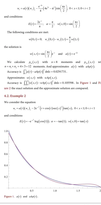
4.2. Example 2
We consider the equation
( )( )
2(
( ) ( )
2)
( )
2e t cos sec tan , 0 1; 0 1
t x x
w =a t w − − t+ t x x < <x < <t
and conditions
( )
2(
( )
)
( )
( )
( )
e t log cos 1 ; tan 1 ; , 0 tan
[image:10.595.193.530.58.744.2]E t = − − α= − w x = x
DOI: 10.4236/am.2018.93017 233 Applied Mathematics Figure 2. w x t
( )
, and wAp x t( )
, .The following conditions are met:
( )
0, 0; x( )
0, x( )
1, tan 1( ) ( )
1,w t = w t −w t = − w t
the solution is
( )
sin( )
( )
2( )
( )
, e and cos
cos
t
x
w x t a t t
x −
= =
We calculate p1n
( )
x t, with n=5 moments and p2n( )
x t, with1 2 3 3 9
n= × = × =n n moments. And approximates a t
( )
with aAp t( )
.Accuracy is 1
( )
( )
20 a t −aAp t d dt x=0.0445868
∫
.Approximates w x t
( )
, with wAp x t( )
, .Accuracy is 1 1
( )
( )
20 0 w x t, −wAp x t, d dt x=0.0502999
∫ ∫
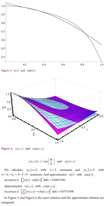
.In Figure 3 and Figure 4 the exact solution and the approximate solution are
compared.
4.3. Example 3
We consider the equation
( )( )
2e cos π π 2sin π , 0 1; 0 16 6 6
t t x x
t x t
w =a t w − − − < <x < <t
and conditions
( )
1cos π ; 2;( )
, 0 23 6
t
E t = α = − w x =x
The following conditions are met:
( )
0, 0; x( )
0, x( )
1, 2( )
1,w t = w t −w t = − w t
DOI: 10.4236/am.2018.93017 234 Applied Mathematics Figure 3. a t
( )
and aAp t( )
.Figure 4. w x t
( )
, and wAp x t( )
, .( )
2 π( )
, cos and e
6
t
t
w x t =x a t = −
We calculate p1n
( )
x t, with n=5 moments and p2n( )
x t, with1 2 3 3 9
n= × = × =n n moments. And approximates a t
( )
with aAp t( )
.Accuracy is 1
( )
( )
20 a t −aAp t d dt x=0.0443166
∫
.Approximates w x t
( )
, with wAp x t( )
, .Accuracy is 1 1
( )
( )
20 0 w x t, −wAp x t, d dt x=0.0731498
∫ ∫
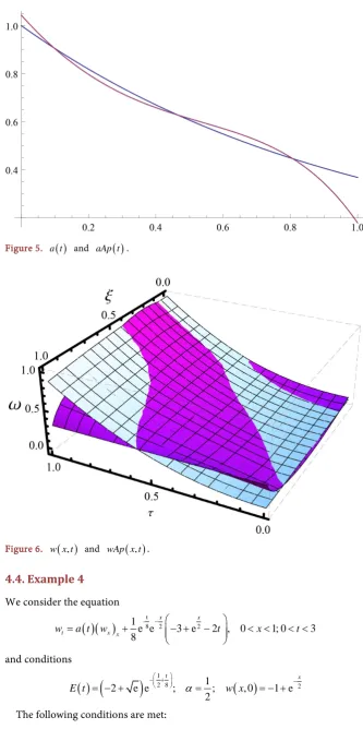
.In Figure 5 and Figure 6 the exact solution and the approximate solution are
DOI: 10.4236/am.2018.93017 235 Applied Mathematics Figure 5. a t
( )
and aAp t( )
.Figure 6. w x t
( )
, and wAp x t( )
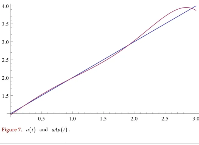
, .4.4. Example 4
We consider the equation
( )( )
-t8 2 2
1
e e 3 e 2 , 0 1; 0 3
8
x x
t x x
w =a t w + − − + − t < <x < <t
and conditions
( )
(
2 e e)
12 8 ; 1;( )
, 0 1 e 22
t x
E t α w x
− + −
= − + = = − +
DOI: 10.4236/am.2018.93017 236 Applied Mathematics
( )
( )
( )
1( )
0, 0; 0, 1, 1,
2
x x
w t = w t −w t = w t
the solution is
( )
, e 2 1 e 8 and( )
1t x
w x t = − − − a t = +t
We calculate p1n
( )
x t, with n=7 moments and p2n( )
x t, with1 2 3 4 12
n= × = × =n n moments.
And approximates a t
( )
with aAp t( )
.Accuracy is 3
( )
( )
20 a t −aAp t dt=0.159805
∫
.Approximates w x t
( )
, with wAp x t( )
, .Accuracy is 1 3
( )
( )
20 0 w x t, −wAp x t, d dt x=Exactitud=0.0354934
∫ ∫
.In Figure 7 and Figure 8 the exact solution and the approximate solution are
compared.
5. Conclusions
We consider the problem of finding a t
( )
and w x t( )
, such that( )( )
( )
,t x x
w =a t w +r x t
under the initial condition w x
( )
, 0 =ϕ( )
x and the boundary conditions( )
0, 0w t = and wx
( )
0,t =wx( )
1,t +α
w( )
1,t about a region( )
{
, , 0 1, 0}
D= x t < <x < <t T . In addition it must be fulfilled 1
( )
( )
0w x t, dx=E t∫
where ϕ
( )
x , r x t( )
, and E t( )
are known functions and α is an arbitraryreal number other than zero. We also assume that the underlying space is
( )
2 L D .
First we find an exact expression for a t w
( ) ( )
1,t . Then, we wrote( )
( ) ( )
* , ,
w x t =a t w x t , and we resolve the integral equation in a first step in
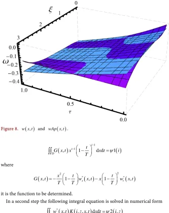
[image:14.595.204.536.500.741.2]numerical form
DOI: 10.4236/am.2018.93017 237 Applied Mathematics Figure 8. w x t
( )
, and wAp x t( )
, .( )
1 1( )
, 1 d d 1
i i
D
t
G x t x x t i
T ψ
−
− − =
∫∫
where
( )
, 2 1 *( )
, 1 2 *( )
,x t
x t t
G x t w x t x w x t
T T T
= − − − −
it is the function to be determined.
In a second step the following integral equation is solved in numerical form
( ) (
)
( )
*
, , , , d d 2 ,
Dw x t K i z x t x t=
ψ
i z∫∫
with *
( )
,
w x t is the unknown function, ψ2 ,
( )
i z is an expression in functionof G x t
( )
, with K i z x t(
, , ,)
known.Both integral equations are solved numerically by applying the moment prob-lems techniques.
Then we find an approximation for a t
( )
; with this approximation we write( )
,aAp x t , using the solution found in the second step and condition
( )
( )
1
0w x t, dx=E t
∫
.We write this approximation aAp x t
( )
, . Finally we find an approximation for( )
,w x t using the solution found in the second step and aAp x t
( )
, .References
DOI: 10.4236/am.2018.93017 238 Applied Mathematics [2] Liao, W., Dehghan, M. and Mohebbi, A. (2009) Direct Numerical Method for an
Inverse Problem of a Parabolic Partial Differential Equation. Journal of Computa-tional and Applied Mathematics, 232, 351-360.
https://doi.org/10.1016/j.cam.2009.06.017
[3] Cannon, J.R., Lin, Y. and Wang, S. (1991) Determination of a Control Parameter in a Parabolic Partial Differential Equation. Journal of the Australian Mathematical Society Series B, 33, 149-163.https://doi.org/10.1017/S0334270000006962
[4] Huzyk, N. (2014) Inverse Problem of Determining the Coefficients in a Degenerate Parabolic Equation. Electronic Journal of Differential Equations, 2014, 1-11. [5] Wang, B.Y., Liao, A.P. and Liu, W. (2012) Simultaneous Determination of
Un-known Two Parameters in Parabolic Equation. International Journal of Applied Mathematics and Computation, 4, 332-336.
[6] Biazar, J. and Houlari, T. (2015) Implementation of Sinc-Galerkin on Parabolic In-verse Problem with Unknown Boundary Condition. International Journal of Indus-trial Mathematics, 7, 313-319.
[7] Dehghan, M. and Tatari, M. (2006) Determination of a Control Parameter in a One-Dimensional Parabolic Equation Using the Method of Radial Basis Functions.
Mathematical and Computer Modelling, 44, 1160-1168.
https://doi.org/10.1016/j.mcm.2006.04.003
[8] Kanca, F. (2017) Determination of a Diffusion Coefficient in a Quasilinear Parabol-ic Equation. Open Mathematics, 15, 77-91.https://doi.org/10.1515/math-2017-0003 [9] Kanca, F. (2016) Inverse Coefficient Problem for a Second-Order Elliptic Equation
with Nonlocal Boundary Conditions. Mathematical Methods in the Applied Sciences, 39, 3152-3158.https://doi.org/10.1002/mma.3759
[10] Grimmonprez, M. and Slodika, M. (2015) A Nonlinear Parabolic Integro-Differential Problem with an Unknown Dirichlet Boundary Condition. Journal of Computa-tional and Applied Mathematics, 275, 421-432.
https://doi.org/10.1016/j.cam.2014.04.022
[11] Hussein, M.S., Lesnic, D. and Ismailov, M.I. (2016) An Inverse Problem of Finding the Time-Dependent Diffusion Coefficient from an Integral Condition. Mathemat-ical Methods in the Applied Sciences, 39, 963-980.
https://doi.org/10.1002/mma.3482
[12] Pintarelli, M.B. (2017) A Problem of Coefficient Determination in Parabolic Equa-tions Solved as Moment Problem. International Journal of Applied Mathematical Research, 6, 109-114.https://doi.org/10.14419/ijamr.v6i4.8319
[13] Akheizer, N.I. (1965) The Classical Moment Problem. Olivier and Boyd, Edinburgh. [14] Akheizer, N.I. and Krein, M.G. (1962) Some Questions in the Theory of Moment.
American Mathematical Society, Providence, RI.
[15] Shohat, J.A. and Tamarkin, J.D. (1943) The Problem of Moments. Mathematical Surveys, American Mathematical Society, Providence, RI.
https://doi.org/10.1090/surv/001
[16] Talenti, G. (1987) Recovering a Function from a Finite Number of Moments. In-verse Problems, 3, 501-517.https://doi.org/10.1088/0266-5611/3/3/016
[17] Ang, D.D., Gorenflo, R., Le, V.K. and Trong, D.D. (2002) Moment Theory and Some Inverse Problems in Potential Theory and Heat Conduction. Lectures Notes in Mathematics, Springer-Verlag, Berlin.https://doi.org/10.1007/b84019
DOI: 10.4236/am.2018.93017 239 Applied Mathematics 253-274.
[19] Pintarelli, M.B. and Vericat, F. (2011) Bi-Dimensional Inverse Moment Problems.
Far East Journal of Mathematical Sciences, 54, 1-23.
[20] Pintarelli, M.B. (2015) Linear Partial Differential Equations of First Order as Bi-Dimensional Inverse Moment Problem. Applied Mathematics, 6, 979-989.
https://doi.org/10.4236/am.2015.66090