ORIGINAL RESEARCH
FUNCTIONAL
Applicability of the Sparse Temporal Acquisition Technique in
Resting-State Brain Network Analysis
X N. Yakunina, T.S. Kim, W.S. Tae, S.S. Kim, andXE.C. Nam
ABSTRACT
BACKGROUND AND PURPOSE: The ability of sparse temporal acquisition to minimize the effect of scanner background noise is of utmost importance in auditory fMRI; however, it has considerably lower temporal efficiency and resolution than the conventional continuous acquisition method. The purpose of this study was to determine whether sparse sampling could be applied to resting-state research by comparing its results with those obtained by using continuous acquisition.
MATERIALS AND METHODS: We identified resting-state networks by using independent component analysis and measured their func-tional connectivity strength in 14 healthy subjects who underwent two 6-minute sparse (60 volumes) and continuous (360 volumes) imaging sessions. To account for the sample size difference, an additional continuous dataset was generated by temporally matching the contin-uous dataset to 60 volumes of the sparse dataset.
RESULTS:Consistent resting-state network maps were produced through all 3 datasets. Scanner background noise did not appear to affect the spatial constitution of the networks, whereas a larger sample size influenced it substantially. The strength of the intranetwork connectivity was similar through the 3 datasets.
CONCLUSIONS: Our results indicated that continuous acquisition is a recommended technique that should be applied in most of the resting-state studies due to its superior temporal efficiency and increased statistical power. The use of sparse temporal acquisition should be restricted to very particular conditions when continuous scanner noise is unacceptable.
ABBREVIATIONS:CA⫽continuous acquisition; DMN⫽default mode network; RSN⫽resting-state network; SBN⫽scanner background noise; STA⫽sparse temporal acquisition; ICA⫽independent component analysis
R
esting-state fMRI may be a better alternative for studying mechanisms that underlie certain auditory disorders than stimulation-based studies. For example, in the case of tinnitus, it may be preferred to investigate spontaneous brain activity in the absence of any external auditory stimulation when tinnitus ismore prominent because no acoustic masking or distraction is present. A few recent studies examined resting-state functional connectivity in patients with tinnitus; however, all of the studies used the conventional continuous acquisition (CA) method, which constantly produces scanner background noise (SBN) and may mask tinnitus acoustically or may even cause residual inhi-bition for several minutes.1-4
Sparse temporal acquisition (STA), in contrast, reduces the effect of SBN by using long interacquisition intervals, which al-lows hemodynamic response induced by acquisition noise to de-cay completely or close to baseline at the time of the next image acquisition.5Practical use of STA in resting-state research has
barely been explored. The trade-off required to minimize the SBN effect by using the STA approach is a lower temporal efficiency that allows substantially fewer volumes to be obtained within a limited imaging time, which could affect the analysis of functional maps and functional connectivity. Questions such as whether STA can provide resting-state results comparable with those widely and consistently obtained to date by using CA techniques and, if the results are different, whether the discrepancy is due to
Received November 1, 2014; accepted after revision August 17, 2015.
From the Institute of Medical Science (N.Y.), Department of Radiology (S.S.K.), and Department of Otolaryngology (E.C.N.), Kangwon National University, School of Medicine, Chuncheon, Republic of Korea; and Neuroscience Research Institute (N.Y., W.S.T., S.S.K., E.C.N.) and Department of Otolaryngology (T.S.K.), Kangwon National University Hospital, Chuncheon, Republic of Korea.
This research was supported by the Basic Science Research Program through the National Research Foundation of Korea, funded by the Ministry of Education (2014R1A1A4A01003909).
Please address correspondence to Eui-Cheol Nam, MD, Department of Otolaryn-gology, School of Medicine, Kangwon National University, One Kangwondaehak-gil, Chuncheon, Kangwon-do, 200-701, Republic of Korea; e-mail: birdynec@ kangwon.ac.kr
Indicates open access to non-subscribers at www.ajnr.org
Indicates article with supplemental on-line tables.
Indicates article with supplemental on-line photos.
the SBN effect or differences in sample size between the 2 acqui-sition methods, remain unanswered.
In this study, we separated the effects of SBN and sample-size differences when comparing the STA and CA techniques. Specif-ically, we compared resting-state networks (RSNs) obtained by the 2 acquisition methods in terms of spatial map constitution and intranetwork functional connectivity strength to establish the applicability of STA to fMRI studies that explore auditory patho-physiology related to alterations in the brain resting state, such as tinnitus or other forms of auditory hyperactivity, in which the noisy environment of CA is unacceptable.
MATERIALS AND METHODS
SubjectsThis study was approved by the institutional review board of Kangwon National University Hospital. All the subjects gave writ-ten informed consent before participation in this study. Fourteen healthy subjects (mean age, 30.6⫾4.7 years; all right-handed; 8 men) with normal hearing (⬍20 dB hearing level in a standard audiometric frequency range of 250 – 8000 Hz) participated in the study. The subjects had no known auditory, neurologic, or neu-ropsychologic disorders. Before the fMRI session, all the subjects underwent pure-tone audiometry and were examined for loud-ness discomfort level and dynamic range.
Data Acquisition
Imaging was performed by using a 3T MR imaging scanner (Achieva TX; Philips Healthcare, Best, the Netherlands) with a 32-channel SENSE head coil. Coronal 3D T1-weighted high-res-olution structural images of the whole brain were acquired for anatomic orientation (TR, 9.8 milliseconds; TE, 4.8 milliseconds; flip angle, 8°; section thickness, 1.0 mm; matrix, 256⫻256⫻195; FOV, 220⫻220 mm; voxel size, 0.94⫻0.94 mm). T2*-weighted functional images were acquired by using a gradient EPI sequence (30 oblique coronal sections; TE, 35 milliseconds; flip angle, 90°; section thickness, 5 mm, with a 1-mm gap; matrix, 80⫻80; FOV, 220⫻220 mm; voxel size, 2.75⫻2.75 mm). The 19th anterior-most section was positioned to intersect the inferior colliculi and the cochlear nuclei in the brain stem. Each subject underwent four 6-minute resting-state runs: 2 continuous (TR, 2 seconds; 180 vol-umes per run; acquisition time, 1.88 seconds; no silent gap between
acquisitions) and 2 sparse (TR, 12 seconds; 30 volumes per run; ac-quisition time, 1.88 seconds; functional acac-quisitions separated by ap-proximately 10-second silent periods free of scanner noise). The sub-jects were instructed to rest quietly with their eyes closed. The subjects wore a protective headset that helped to diminish SBN from the original level of 115 dB sound pressure level to 95 dB sound pressure level. The scanner coolant pump was turned off during im-aging to further reduce the ambient noise level.
Data Preprocessing
Preprocessing was performed by using the SPM12 software pack-age (http://www.fil.ion.ucl.ac.uk/spm/software/spm12) in the Mat-lab 7.8 programming environment (MathWorks, Natick, Massachu-setts). In each run, the functional images were corrected for head motion, coregistered, normalized to the standard Montreal Neuro-logical Institute T1 template, and spatially smoothed with an 8-mm isotropic Gaussian kernel. Section timing correction was not per-formed because of the discontinuous nature of the STA data.
Independent Component Analysis
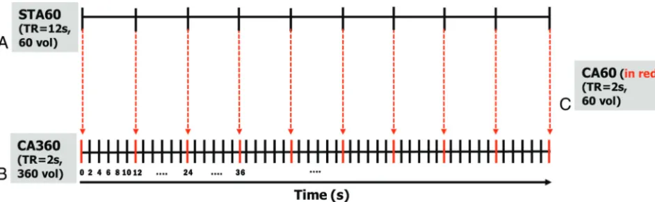
To eliminate the effect of the difference in sample sizes between the STA dataset (60 volumes, labeled STA60) and CA dataset (360 volumes, labeled CA360), a third matched continuous dataset (CA60) was created by selecting 60 volumes of the CA360 set, which corresponded in time to the STA60 dataset volumes (Fig 1). Three pairs of datasets were compared. The STA60 and CA60 datasets were compared to assess any SBN effect, because they had equal numbers of volumes. A comparison of the CA60 and CA360 datasets was performed to reveal the effect of sample size, because they were equal in terms of continuous SBN effect and differed only in sample size. Finally, the STA60 and CA360 datasets were compared directly.
Spatial independent component analysis (ICA) was per-formed by using the Group ICA of fMRI Toolbox software (GIFT, ver. 2.0a; http://mialab.mrn.org/software/gift/).6The ICA order
of 33, approximately half of the full temporal dimension of the STA60 and CA60 data, was chosen so as not to overfit the model.7,8 Group ICA was assessed for concatenated
STA60-CA60, CA60-CA360, and STA60-CA360 datasets. Independent components were extracted by using the Infomax algorithm. Twenty iterations of ICA were performed by using the ICASSO
[image:2.594.57.528.47.192.2]algorithm to verify the stability of the components.9All individual
components were scaled to represent percentage signal change. Group statistical maps of each component were generated by per-forming a voxelwise 1-samplettest on these individual indepen-dent component maps and then thresholded at false discovery rate corrected at q⬍0.05.
The resulting group components for each dataset were subse-quently visually examined to determine their neural or artifactual nature. Components were considered to be gray matter compo-nents (RSN) if they were found in clusters that matched well with particular gray matter structures rather than being diffusely scat-tered across large regions or found in the periphery.
Statistical Comparison of RSN Spatial Maps and Their Characteristics
To compare the results of individual analyses, a pairedttest was performed on individual RSN maps of STA60-CA60, CA60-CA360, and STA60-CA360 analyses. T-contrasts of STA60⬎ CA60 and CA60⬎STA60 were performed to explore the effect of SBN; t-contrasts of CA360⬎CA60 and CA60⬎CA360 were performed to explore the effect of volume number. T-contrasts of STA60⬎CA360 and CA360-STA60 were performed to see how the 2 acquisition methods compared directly. Contrast maps were thresholded at the false discovery rate corrected q⬍0.05.
Statistical analyses were performed by using SPSS software (ver. 19.0; IBM, Armonk, New York). The number of voxels, average percentage signal change, and maximum percentage signal change were calculated for each individual RSN of each pair-wise ICA and compared between STA60 and CA60, CA60 and CA360, and STA60 and CA360 by using the Wilcoxon signed rank test with Bonferroni correction for multiple comparisons.
Functional Connectivity Analysis
Intranetwork RSN functional connectivity strength, another measure of compositional robustness, was compared between the 3 dataset pairs. Connectivity was assessed between ROIs placed in major subregions of each RSN from each dataset. Each RSN was divided into spatially nonoverlapping subareas (eg, left/right, frontal/parietal, left (right)/medial), which resulted in several pairs of coupled subregions. The peak voxel of each subarea was used to create ROIs. ROIs were created as spheres of 3-mm radius. Center voxels for ROIs for each dataset pair comparison were chosen as peak voxels of group ICA maps performed on the cor-responding concatenated datasets.
Connectivity analysis was performed by using the CONN functional connectivity toolbox, Version 15.010; http://www.
nitrc.org/projects/conn) with the CompCor method for estimat-ing and removestimat-ing physiologic and other sources of noise.11The
individual motion parameters and a linear term for detrending were included as covariates. The residual blood-oxygen level de-pendent signal was bandpass-filtered over a low-frequency win-dow of interest (0.01– 0.1 Hz). For each dataset and for each ROI, time courses were extracted and averaged over all voxels in the ROI. Pearson correlation coefficients were calculated between the time courses of each pair of ROIs for every subject. Correlation coefficients and correlation maps were converted to Fisher z scores and compared pair-wise between STA60 and CA60, CA60
and CA360, and STA60 and CA360 by using a Wilcoxon signed rank test with the Bonferroni correction.
Frequency Domain Analysis
To assess the fundamental fluctuation frequency of each RSN from the CA360 dataset and to determine whether it fell within the frequency range covered by STA with its lower sampling rate, a fast Fourier transform was performed on each RSN time course produced by ICA to obtain its frequency power spectrum. Before performing the Fourier transform, a Butterworth high-pass filter was applied to all time courses, with a lower cutoff frequency of 0.01 Hz.
RESULTS
Independent Component Analysis
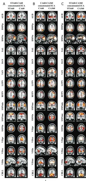
All independent components of all 3 datasets had very high sta-bility indices (mean STA60-CA60, 0.948⫾0.055; CA60-CA360, 0.972 ⫾0.01; STA60-CA360, 0.975⫾ 0.072). Fourteen RSNs were obtained consistently from the 3 concatenated analyses of paired datasets: auditory, 2 default mode networks (DMNs), sa-lience, dorsal and ventral attentional, 2 frontoparietal, 2 sensori-motor, 3 visual, and cerebellar networks. An additional anterolat-eral sensorimotor network was produced by STA60-CA60 and STA60-CA360 analyses, and a medial visual network was, in ad-dition, found in CA60-CA360 analysis, which made a total of 15 discovered RSNs in all 3 dataset pairs (Fig 2; On-line Table 1).
Statistical Comparison of RSN Spatial Maps and Characteristics
A comparison of the STA60 and CA60 individual spatial maps revealed a larger auditory network in STA60. A comparison of CA60 and CA360 revealed greater salience, right frontoparietal, and 3 visual networks in the CA360 dataset. A comparison of STA60 and CA360 revealed greater posterior and anterior DMN and lateral visual networks in CA360 (On-line Fig 1).
The 3 investigated RSN characteristics (number of voxels, av-erage and maximum percentage signal changes), a comparison of STA60 to CA60 revealed a greater voxel number for the posterior DMN in CA60. In CA60-CA360 comparison, the CA360 dataset consistently displayed significantly greater values than CA60 for several RSNs, including salience, frontoparietal, sensorimotor, and visual networks. A comparison of STA60 with CA360 showed a greater voxel number for the anterior and posterior DMN in CA360 (On-line Table 2).
Functional Connectivity Analysis
Stronger connectivity of the medial sensorimotor network was observed in STA60 compared with CA60; CA360 showed a more robust posterior DMN compared with CA60 and compared with STA60 (Table).
Frequency Domain Analysis
DISCUSSION
The issue of SBN effects on the resting state of the brain remains poorly explored. To date, 2 reported studies evaluated the SBN effect on the resting state. Rondioni et al12used a “silent” EPI sequence,
which allowed reduction of SBN by only approximately 12 dB. Al-though quieter than the original EPI SBN level, this does not seem to provide an adequately “silent” environment suitable for auditory studies. In our study, STA provided approximately 10-second com-pletely silent periods between consecutive image acquisitions, whereas SBN was generated continuously during CA sessions. An-other study used STA in comparison with the CA technique for rest and auditory task conditions.13Although the researchers used ICA as
in this study, there were significant differences: first, we observed and included into the analysis substantially more RSNs for comparison; second, we eliminated the influence of a greater sample size of CA by creating the volume-matched CA60 dataset.
ICA successfully extracted consistent canonical RSNs identi-fied by previous resting-state and task-based studies for each pair of datasets.14-17Except for an anterolateral sensorimotor network
in STA60-CA60 and STA60-CA360 analyses, and the medial vi-sual network in CA60-CA360 analysis, all identified RSNs matched across the 3 dataset pairs. RSNs identified from all data-set pairs included most of the RSNs provided as templates with the GIFT software18and RSNs identified by a multisubject
high-or-der ICA study.17All components were highly stable.
A comparison of the STA60 with the CA60 dataset revealed the larger number of voxels for the posterior DMN in CA60 (On-line Table 2). No other differences were found, either in spatial RSN characteristics or in the intranetwork functional connectivity ( Ta-ble). Therefore, SBN did not seem to affect RSNs significantly.
The CA360 dataset, however, was significantly larger than CA60 in terms of the voxel number and average and maximum percent-age signal changes for a number of networks. These results were in line with the comparison of RSN spatial maps, in which the same RSNs had a significantly greater spatial extent in CA360 than those in CA60 (On-line Fig 1). This could indicate that the larger sample size of CA360 had a substantial effect on the spatial distri-bution of the ICA components. However, the sample size did not appear to have any impact on functional connectivity because no differences between the 2 datasets were found.
Direct comparison of the STA60 with the CA360 dataset re-vealed a larger number of voxels in the anterior and posterior DMN in CA360 (which agreed with the results of the spatial maps comparison) (On-line Table 2; On-line Fig 1). CA360 also dem-onstrated stronger functional connectivity for the posterior DMN (Table). Because the effects of SBN and sample size were not sep-arated here, it is unclear how much either was responsible for this difference. Although a larger sample size appeared to have a stron-ger influence on ICA results after the results of CA60-CA360 com-parison, the posterior DMN demonstrated a higher voxel number in CA60 compared with STA60, which means that a larger DMN in CA360 may also be due to the SBN effect. The brain switches into the default mode of ongoing introspective activity when it is not engaged in any immediate attention-demanding task or stim-ulation.19,20In fMRI resting-state studies, there is no active task or
stimulus to voluntarily direct attention, which can result in atten-tion being involuntarily drawn to SBN.
Continuous SBN in CA, if recognized as a constant but mean-ingless and harmless sensory stimulus, would lead to attention system fatigue and send top-down controlling signals to the
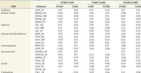
pe-Intranetwork functional connectivitya
RSN Notation
STA60-CA60 CA60-CA360 STA60-CA360
STA60 CA60 CA60 CA360 STA60 CA360
Auditory AUD_LR 0.17 0.16 0.12 0.25 0.21 0.14
Default mode DMNp_ML ⫺0.04 0.07 0.18 0.25 0.08 0.11
DMNp_MR ⫺0.02 0.04 0.14 0.12 ⫺0.03 0.04
DMNp_LR 0.20 0.29 0.19 0.26 0.15 0.33b
DMNa_FP 0.19 0.19 0.18 0.26 0.23 0.25
Salience SAL_ML 0.13 0.23 0.19 0.15 0.26 0.26
SAL_MR 0.21 0.23 0.03 0.08 0.21 0.27
SAL_LR 0.27 0.26 ⫺0.02 ⫺0.02 0.20 0.25
Dorsal/ventral attention DAN_LR 0.19 0.29 0.20 0.29 0.36 0.36
VAN_ML 0.27 0.33 0.19 0.24 0.06 0.16
VAN_MR 0.07 0.12 0.20 0.25 0.22 0.31
VAN_LR 0.01 0.11 0.09 0.16 0.29 0.37
Frontoparietal RFPN_FP 0.25 0.11 0.28 0.31 0.09 0.22
LFPN_FP ⫺0.06 ⫺0.07 0.04 0.00 0.07 0.17
Sensorimotor SMNala_LR 0.31 0.13 – – 0.37 0.27
SMNme_LR 0.25 0.11 0.27 0.28 0.21 0.23
SMNla_LR 0.02 ⫺0.01 0.03 0.13 0.28 0.31
VISpr_LR 0.37 0.41 0.03 0.13 0.68 0.74
Visual VISex_LR 0.39 0.40 0.02 0.06 0.34 0.28
VISla_LR 0.27 0.34 0.08 0.15 0.40 0.49
VISme_LR – – 0.39 0.44 – –
Cerebellum CBLL_LR 0.01 ⫺0.02 0.05 0.06 0.13 0.04
Note:—L indicates left; R, right; M, medial; F, frontal; P, posterior; AUD, auditory; DMNp/a, default mode posterior/anterior; SAL, salience; DAN/VAN, dorsal/ventral attentional; RFPN/LFPN, right/left frontoparietal; SSMala/me/la, sensorimotor anteromedial/medial/lateral; VISpr/ex/la/me, visual primary/extrastriate/lateral/medial; CBLL, cerebellar networks.
a
Correlation coefficients between subareas of each RSN were compared for presenting SBN effect (STA60-CA60 comparison), sample size effect (CA60-CA360 comparison), and the direct comparison of the 2 acquisition methods (STA60-CA360 comparison).
b
[image:5.594.54.532.55.305.2]ripheral auditory system to discontinue responding.21Decreased
attention and adaptation (fatigue) to the continuous stimulus (SBN) in CA may result in increased activity in the default mode network. In contrast, the far sparser occurrence of SBN in STA, similar to auditory oddball or novelty stimulation, might evoke an attentional response, which, subsequently, may keep subjects more alert and result in disturbed default mode activity. Note that this might not be the case with task-oriented studies, in which allocation of attentional resources is largely governed by the task at hand, and SBN may not impact attentional and default mode networks in the same manner as in the resting state. Furthermore, although the de-scribed mechanism related to regulation of attention by SBN is one possible explanation, other scenarios may exist and should not be ruled out.
Frequency analysis showed that the dominant frequency of all RSNs (which is known to be⬍0.1 Hz22,23) was lower than the
Ny-quist frequency of the STA’s sampling rate (0.0417 Hz), which indi-cated that the low sampling rate of STA was fast enough to capture low-frequency fluctuations of resting brain networks. However, some components of CA360 had frequencies beyond the Nyquist frequency, which had a comparably strong power. It means that some essential information about temporal dynamics could still be lost in STA, which is a method far inferior to CA for studying tem-poral behavior of the brain because of its discontinuous nature.
Altogether, SBN did not seem to have any effect on RSN spatial maps and connectivity, except possibly disturbing DMN activity. Thus, CA should be a preferred method of acquisition in general resting-state studies due to its superior temporal resolution, in-creased statistical power, and less subject-to-subject variability. STA, however, did not appear to have any benefits compared with CA. Its disadvantages, such as increased variability, temporal dis-continuity, small sample size, and decreased power, make it a far inferior method to CA. STA may be applicable only in very rare and particular cases, such as when continuous SBN may mask tinnitus or is unbearable by patients with hyperacusis or other auditory disorders.
Regarding the limitations of the current study, it should be noted that SBN may not be the only difference factor between STA60 and CA60 datasets. The 2 datasets may differ in signal-to-noise ratio because the longer interacquisition intervals in STA allow for better T1 recovery and thus greater signal intensity.5
CONCLUSIONS
STA was able to extract the same networks as CA, but it did not display any advantages over the continuous method. SBN did not seem to affect either spatial maps or connectivity of the RSNs. Therefore, apart from very particular cases when continuous SBN is unwanted or unbearable, CA is a recommended acquisition method for most of the resting-state studies, including those of auditory disorders, due to its eminent temporal resolution and high statistical power.
REFERENCES
1. Maudoux A, Lefebvre P, Cabay JE, et al.Auditory resting-state net-work connectivity in tinnitus: a functional MRI study.PLoS One 2012;7:e36222CrossRef Medline
2. Ueyama T, Donishi T, Ukai S, et al.Brain regions responsible for tinnitus distress and loudness: a resting-state FMRI study.PLoS One2013;8:e67778CrossRef Medline
3. Schmidt SA, Akrofi K, Carpenter-Thompson JR, et al.Default mode, dorsal attention and auditory resting state networks exhibit differ-ential functional connectivity in tinnitus and hearing loss.PLoS One2013;8:e76488CrossRef Medline
4. Burton H, Wineland A, Bhattacharya M, et al.Altered networks in bothersome tinnitus: a functional connectivity study.BMC Neuro-sci2012;13:3CrossRef Medline
5. Hall DA, Haggard MP, Akeroyd MA, et al.“Sparse” temporal sam-pling in auditory fMRI.Hum Brain Mapp1999;7:213–23Medline
6. Calhoun VD.Group ICA of fMRI toolbox (GIFT).2004. http:// mialab.mrn.org/software/. Accessed October 15, 2015.
7. Abou Elseoud A, Littow H, Remes J, et al.Group-ICA model order highlights patterns of functional brain connectivity.Front Syst Neu-rosci2011;5:37CrossRef Medline
8. Kiviniemi V, Starck T, Remes J, et al.Functional segmentation of the brain cortex using high model order group PICA.Hum Brain Mapp 2009;30:3865– 86CrossRef Medline
9. Himberg J, Hyvarinen A.Icasso: software for investigating the reli-ability of ICA estimates by clustering and visualization.In: Proceed-ings of the IEEE 13th Workshop on Neural Network for Signal Process-ing, Toulouse, France. May 17–19, 2003: 259 – 68
10. Whitfield-Gabrieli S, Nieto-Castanon A.Conn: a functional connec-tivity toolbox for correlated and anticorrelated brain networks. Brain Connect2012;2:125– 41CrossRef Medline
11. Behzadi Y, Restom K, Liau J, et al.A component based noise correc-tion method (CompCor) for BOLD and perfusion based fMRI. Neu-roimage2007;37:90 –101CrossRef Medline
12. Rondinoni C, Amaro E Jr, Cendes F, et al.Effect of scanner acoustic background noise on strict resting-state fMRI.Braz J Med Biol Res 2013;46:359 – 67CrossRef Medline
13. Langers DR, van Dijk P.Robustness of intrinsic connectivity net-works in the human brain to the presence of acoustic scanner noise. Neuroimage2011;55:1617–32CrossRef Medline
14. Beckmann CF, DeLuca M, Devlin JT, et al.Investigations into rest-ing-state connectivity using independent component analysis. Phi-los Trans R Soc Lond B Biol Sci2005;360:1001–13CrossRef Medline
15. Damoiseaux JS, Rombouts SA, Barkhof F, et al.Consistent resting-state networks across healthy subjects.Proc Natl Acad Sci U S A 2006;103:13848 –53CrossRef Medline
16. De Luca M, Beckmann CF, De Stefano N, et al.fMRI resting state networks define distinct modes of long-distance interactions in the human brain.Neuroimage2006;29:1359 – 67CrossRef Medline
17. Allen EA, Erhardt EB, Damaraju E, et al.A baseline for the multivar-iate comparison of resting-state networks.Front Syst Neurosci2011; 5:2CrossRef Medline
18. Shirer WR, Ryali S, Rykhlevskaia E, et al.Decoding subject-driven cognitive states with whole-brain connectivity patterns.Cereb Cor-tex2012;22:158 – 65CrossRef Medline
19. Raichle ME, Snyder AZ.A default mode of brain function: a brief history of an evolving idea.Neuroimage2007;37:1083–90; discussion 1097–99CrossRef Medline
20. Buckner RL, Andrews-Hanna JR, Schacter DL.The brain’s default network: anatomy, function, and relevance to disease.Ann N Y Acad Sci2008;1124:1–38CrossRef Medline
21. Guinan JJ Jr.Cochlear efferent innervation and function.Curr Opin Otolaryngol Head Neck Surg2010;18:447–53CrossRef Medline
22. Greicius MD, Krasnow B, Reiss AL, et al.Functional connectivity in the resting brain: a network analysis of the default mode hypothe-sis.Proc Natl Acad Sci U S A2003;100:253–58CrossRef Medline