University of Warwick institutional repository: http://go.warwick.ac.uk/wrap
A Thesis Submitted for the Degree of PhD at the University of Warwick
http://go.warwick.ac.uk/wrap/61310
This thesis is made available online and is protected by original copyright.
Please scroll down to view the document itself.
Sequence Distance Embeddings
by
Graham Cormode
Thesis
Submitted to the University of Warwick
for the degree of
Doctor of Philosophy
Computer Science
Contents
List of Figures vi
Acknowledgments viii
Declarations ix
Abstract xi
Abbreviations xii
Chapter 1 Starting 1
1.1 Sequence Distances . . . 2
1.1.1 Metrics . . . 3
1.1.2 Editing Distances . . . 3
1.1.3 Embeddings . . . 3
1.2 Sets and Vectors . . . 4
1.2.1 Set Difference and Set Union . . . 4
1.2.2 Symmetric Difference . . . 5
1.2.3 Intersection Size . . . 5
1.2.4 Vector Norms . . . 5
1.3 Permutations . . . 6
1.3.1 Reversal Distance . . . 7
1.3.2 Transposition Distance . . . 7
1.3.3 Swap Distance . . . 8
1.3.4 Permutation Edit Distance . . . 8
1.3.5 Reversals, Indels, Transpositions, Edits (RITE) . . . 9
1.4 Strings . . . 9
1.4.1 Hamming Distance . . . 10
1.4.2 Edit Distance . . . 10
1.4.3 Block Edit Distances . . . 11
1.5 Sequence Distance Problems . . . 14
1.5.1 Efficient Computation and Communication . . . 14
1.5.2 Approximate Pattern Matching . . . 15
1.5.3 Geometric Problems . . . 16
1.5.4 Approximate Neighbors . . . 16
1.5.5 Clustering for k-centers . . . 17
Chapter 2 Sketching and Streaming 21
2.1 Approximations and Estimates . . . 22
2.1.1 Sketch Model . . . 23
2.1.2 Streaming . . . 23
2.1.3 Equality Testing . . . 24
2.2 Vector Distances . . . 26
2.2.1 Johnson-Lindenstrauss lemma . . . 26
2.2.2 Frequency Moments . . . 27
2.2.3 L1Streaming Algorithm . . . 28
2.2.4 Sketches using Stable Distributions . . . 29
2.2.5 Summary of VectorLpDistance Algorithms . . . 31
2.3 Set Spaces and Vector Distances . . . 32
2.3.1 Symmetric Difference and Hamming Space . . . 32
2.3.2 Set Union and Distinct Elements . . . 35
2.3.3 Set Intersection Size . . . 37
2.3.4 Approximating Set Measures . . . 40
2.4 Geometric Problems . . . 41
2.4.1 Locality Sensitive Hash Functions . . . 41
2.4.2 Approximate Furthest Neighbors for Euclidean Distance . . . 43
2.4.3 Clustering fork-centers . . . 44
2.5 Discussion . . . 45
Chapter 3 Searching Sequences 46 3.1 Introduction . . . 47
3.1.1 Computational Biology Background . . . 47
3.1.2 Results . . . 48
3.2 Embeddings of Permutation Distances . . . 48
3.2.1 Swap Distance . . . 49
3.2.2 Reversal Distance . . . 51
3.2.3 Transposition Distance . . . 53
3.2.4 Permutation Edit Distance . . . 55
3.2.5 Hardness of Estimating Permutation Distances . . . 58
3.2.6 Extensions . . . 62
3.3 Applications of the Embeddings . . . 62
3.3.1 Sketching for Permutation Distances . . . 62
3.3.2 Approximating Pairwise Distances . . . 64
3.3.3 Approximate Nearest Neighbors and Clustering . . . 65
3.3.4 Approximate Pattern Matching with Permutations . . . 67
3.4 Discussion . . . 68
Chapter 4 Strings and Substrings 70 4.1 Introduction . . . 71
4.2 Embedding String Edit Distance with Moves intoL1Space . . . 72
4.2.1 Edit Sensitive Parsing . . . 72
4.2.2 Parsing of Different Metablocks . . . 73
4.2.3 ConstructingET(a) . . . 75
4.3 Properties of ESP . . . 77
4.3.1 Upper Bound Proof . . . 77
4.3.2 Lower Bound Proof . . . 79
4.4.1 Compression Distance . . . 85
4.4.2 Unconstrained Deletes . . . 86
4.4.3 LZ Distance . . . 87
4.4.4 Q-gram distance . . . 88
4.5 Solving the Approximate Pattern Matching Problem for String Edit Distance with Moves 89 4.5.1 Using the Pruning Lemma . . . 89
4.5.2 ESP subtrees . . . 89
4.5.3 Approximate Pattern Matching Algorithm . . . 90
4.6 Applications to Geometric Problems . . . 92
4.6.1 Approximate Nearest and Furthest Neighbors . . . 92
4.6.2 String Outliers . . . 94
4.6.3 Sketches in the Streaming model . . . 95
4.6.4 Approximatep-centers problem . . . 95
4.6.5 Dynamic Indexing . . . 96
4.7 Discussion . . . 97
Chapter 5 Stables, Subtables and Streams 98 5.1 Introduction . . . 99
5.1.1 Data Stream Comparison . . . 99
5.1.2 Tabular Data Comparison . . . 100
5.2 Sketch Computation . . . 102
5.2.1 Implementing Sketching Using Stable Distributions . . . 102
5.2.2 Median of Stable Distributions . . . 103
5.2.3 Faster Sketch Computation . . . 105
5.2.4 Implementation Issues . . . 108
5.3 Stream Based Experiments . . . 109
5.4 Experimental Results for Clustering . . . 113
5.4.1 Accuracy Measures . . . 114
5.4.2 Assessing Quality and Efficiency of Sketching . . . 115
5.4.3 Clustering Using Sketches . . . 118
5.4.4 Clustering Using VariousLpNorms . . . 121
5.5 Discussion . . . 125
Chapter 6 Sending and Swapping 126 6.1 Introduction . . . 127
6.1.1 Prior Work . . . 127
6.1.2 Results . . . 129
6.2 Bounds on communication . . . 130
6.3 Near Optimal Document Exchange . . . 132
6.3.1 Single Round Protocol . . . 132
6.3.2 Application to distances of interest . . . 133
6.3.3 Computational Cost . . . 134
6.4 Computationally Efficient Protocols for String Distances . . . 136
6.4.1 Hamming distance . . . 137
6.4.2 Edit Distance. . . 140
6.4.3 Tichy’s Distance . . . 141
6.4.4 LZ Distance . . . 143
6.4.5 Compression Distances and Edit Distance with Moves . . . 144
6.4.6 Compression Distance with Unconstrained Deletes . . . 147
6.6 Discussion . . . 149
Chapter 7 Stopping 152 7.1 Discussion . . . 153
7.1.1 Nature of Embeddings . . . 153
7.1.2 Permutations and Strings . . . 154
7.2 Extensions . . . 155
7.2.1 Trees . . . 155
7.2.2 Graphs . . . 156
7.3 Further Work . . . 157
Appendix A Supplemental Sectionon Sequence Similarity 159 A.1 Combined Permutation Distances . . . 160
A.1.1 Combining All Operations . . . 160
A.1.2 Transpositions, Insertions, Reversals, Edits and Deletions . . . 160
List of Figures
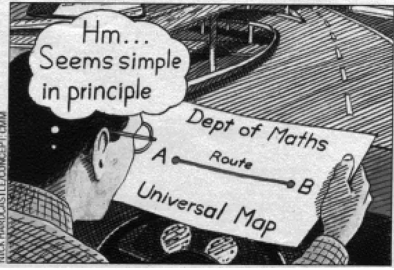
1.1 A map is an embedding of geographic data into the 2D plane with some loss of information 4
1.2 Summary of the distances of interest . . . 18
2.1 Key features of the different methods described in Section 2.2. . . 31
2.2 Approximability of set quantities . . . 41
3.1 There is always a transposition that removes one breakpoint . . . 53
3.2 Illustrating Permutation Edit Distance embedding . . . 56
3.3 Analysing the Longest Increasing Sequence . . . 57
3.4 An exact embedding of Permutation Edit Distance into Hamming distance . . . 59
3.5 A set of permutations that formsK2,3under permutation edit distance . . . 60
3.6 Permutation Edit Distance between the two pairs of possibilities . . . 61
3.7 Summary of the different sequence distance measures . . . 63
4.1 The process of alphabet reduction and landmark finding . . . 74
4.2 Given the landmark characters, the nodes are formed. . . 75
4.3 The hierarchy is formed by repeated application of alphabet reduction and landmark finding 76 4.4 The hierarchical structure of nodes is represented as a parse tree on the stringa. . . 77
4.5 The hierarchical parsing induces a vector representation . . . 81
4.6 For the lower bound proof, we mark nodes that are common to both strings . . . 82
4.7 The first stages of editing the string . . . 83
4.8 The target string is completed . . . 84
4.9 An ESP subtree can be iteratively computed . . . 91
5.1 The value of the median of stable distributions with parameterp <2 . . . 103
5.2 Compound sketches can be formed from four sketches that represent the area required. . 107
5.3 Results for insertions based on a Zipf distribution . . . 110
5.4 Finding the Hamming Norm of Network Data . . . 111
5.5 Testing performance for a sequence of insertions and deletions . . . 112
5.6 Testing performance for a sequence of insertions . . . 113
5.7 Measuring the Hamming distance between network streams . . . 114
5.8 Assessing the distance between20,000randomly chosen pairs . . . 116
5.9 Accuracy results when tiling four sketches to cover a subrectangle . . . 117
5.10 Quality of pairwise comparisons with tiled sketches . . . 118
5.11 Timing results for differentLpdistances . . . 119
5.12 Quality results for differentLpdistances . . . 120
5.13 Clustering with different numbers of means . . . 121
5.14 Varyingpto find a known clustering . . . 122
5.16 Clustering of one day’s call data for the whole United States. . . 124
6.1 Calculating a colour using Hamming codes . . . 135
6.2 Illustrating how Hamming differences affect the binary parse tree . . . 139
6.3 Illustrating how edit differences affect the binary parse tree ofa . . . 142
6.4 The protocol for exchanging strings based on Compression Distance . . . 146
6.5 Main results on document exchange . . . 150
Acknowledgments
Any thesis is more than just the work of one person, and I owe a large debt to many people who have helped me along the way. In particular, I must acknowledge the help of three people who have all made huge contributions to my work.
Mike Paterson has been a great supervisor throughout my years at Warwick. His willingness to help with whatever I came to him with and his meticulous attention to detail have been of immense help. Cenk S.ahinalp introduced me to some marvellous problems, and worked on them together with me with insight and guidance. He also arranged for me to spend a year of my degree with him at Case Western Reserve University. S. Muthukrishnan (Muthu) has always responded with enthusiasm to my work, and together we have had a lot of fun writing papers. He was a superb mentor when I visited AT&T as an intern in Summer 2000, and I’m very grateful to him for arranging frequent trips back to visit since then.
After these three, I must also thank all the other people who have written papers with me since I began my studies: Uzi Vishkin, Nick Koudas, Piotr Indyk, Tekin Ozsoyoglu, Meral Ozsoyoglu, Mayar Datar and Hurkan Balkir. Throughout my studies, I have been very fortunate with my officemates, first amongst these being Jon Sharp, who has been both an officemate and a flatmate. There has also been Mary Cryan, Hesham Al-ammal, Sun Chung, Steven Kelk, and Harish Bhanderi. I also need to thank everyone with whom I’ve talked about my work: Amit Chakrabarti, Funda Ergun, Martin Strauss, and many others. My studies have been supported financially by a University of Warwick Graduate Award; by a Case Western Reserve University Fellowship; by an internship at AT&T research; and by travel grants from the Center for Discrete Mathematics and Theoretical Computer Science (DIMACS); Algorithms and Complexity — Future Technologies (ALCOM-FT); the University of Haifa, Israel; University of Warwick American Study and Student Exchanges Committee (ASSEC); and the Department of Computer Science, University of Warwick.
My family, and especially my parents deserve recognition for putting up with my travails, and for never knowing entirely what it is that I do1. My friends and flatmates, too many to mention, have also been supportive or diverting, and so made my studies easier to manage. Mark Hadley deserves much credit for making available his wthesis LATEXstyle file. I would also like to acknowledge the Students’ Union of the University of Warwick, and in particular the Elections Group, the Postgraduate Committee and the crossword of the Warwick Boar newspaper, all of which have contributed to dragging this thesis out longer than it otherwise needed to take.
Declarations
Unlike Wilde, I have a great deal to declare. Much of the material in this thesis derives from papers that have been published in refereed conferences. These are all collaborative works, and as is the nature of such collaborations, it is often difficult to disentangle or lay claim to the individual efforts of any particular author.
Chapter 1 consists mostly of introductory and background material. Section 1.5.2 derives from an idea of S. Muthukrishnan, described in [CM02]; the remainder is new for this thesis. Chapter 2 consists mostly of a discussion of relevant prior work of other authors (attributed when referenced), which is used by later sections. In particular, the methods described in Section 2.2.4 are due to Indyk. They were outlined in [Ind00], and then expanded upon in [CIKM02] and [CDIM02]. Some of the subsections of Section 2.3.1 is my work from [CDIM02]. The remainder, constituting the bulk of the chapter, is an original presentation of related work.
In Chapter 3, Section 3.1, Section 3.2.2, Section 3.2.3, Section 3.2.4, and Section 3.3 are extended versions of results first shown in [CMS.01]. All the embeddings and related proofs presented there are my own work, as are the hardness results and applications of the embeddings. S. Muthukrishnan sug-gested the application to Approximate Pattern Matching, which I described and analysed. The second example in Section 3.2.1 has been published in another form as 1 Across in [Cor02]. Sections 3.2.1, 3.2.5, 3.2.6 and 3.3.3 is my work that has not previously been published.
The embedding presented in Chapter 4 derives from that given by Cenk Sahinalp in [MS.00], as is discussed in the text. The construction given here is a significantly simplified reformulation, about which it is possible to prove stronger results. The proofs are due to me, as is the application to edit distance with moves. The application to pattern matching and streaming computation were suggested by S. Muthukrishnan, and were again described and analysed by myself. The material in Sections 4.4.2, 4.4.3, 4.4.4, and 4.6 is my own work which has not been published elsewhere. Chapter 5 reports experiments that I designed, coded, ran and analysed myself that were first described in [CIKM02] and [CDIM02]. In Chapter 6, Section 6.2, Section 6.3, Section 6.4.1, Section 6.4.2 and Section 6.4.4 are derived from [CPS.V00]. The entirety of the results in this chapter were discovered and described by me, and the results in Section 6.5 have not previously been published. None of this work is drawn from [OBCO00], but I wanted to mention it anyway.
Sequence Distance Embeddings
The Maze of Ways from A to B
Writing a book is rather like going on a long journey. You know where you are (at the beginning) and you know where you want to get to (the end). The big problem is, what route should you take? I’m sure you know that the shortest distance between two points is a straight line, but if you decide now to go somewhere in a straight line, after going just a few paces you will probably come to a sudden stop and say, ‘Ouch!’ If the pain is in your leg, you will have walked into the furniture, but if the pain is in your nose, you will have walked into the wall. And it’s no good me telling you to stop being stupid and sit down — with your nose right up against the wall, you won’t be able to read this book.
Abstract
Sequences represent a large class of fundamental objects in Computer Science — sets, strings, vectors and permutations are considered to be sequences. Distances between sequences measure their similarity, and computations based on distances are ubiquitous: either to compute the distance, or to use distance computation as part of a more complex problem. This thesis takes a very specific approach to solving questions of sequence distance: sequences are embedded into other distance measures, so that distance in the new space approximates the original distance. This allows the solution of a variety of problems including:
• Fast computation of short ‘sketches’ in a variety of computing models, which allow sequences to be compared in constant time and space irrespective of the size of the original sequences.
• Approximate nearest neighbor and clustering problems, significantly faster than the na¨ıve exact solutions.
• Algorithms to find approximate occurrences of pattern sequences in long text sequences in near linear time.
• Efficient communication schemes to approximate the distance between, and exchange, sequences in close to the optimal amount of communication.
Abbreviations
Sets
A, B SetsAandB A∪B Set Union
A∩B Set Intersection
A∆B Symmetric set difference
|A| Number of distinct elements in setA
χ(A) The characteristic function of a set, mapping a subset of an (ordered) set onto a bit-string — Section 2.3.1
Vectors and Matrices
a,b Vectors
|a| Length (dimensionality) of the vectora ||a||p Lpnorm of the vectora— Definition 1.2.5
||a−b||p Lpdistance between vectorsaandb
||a||H The Hamming norm ofa, the number of locations in which it is non-zero. A,B Matrices
Ai Theith row of matrixA, a vector.
median(a) The median of the multi-set of values in the vectora
sk(a) The sketch of a vectora— Definition 2.1.3
i(a, b) The size of the intersection of two bit-stringsaandb— Definition 1.2.4
Permutations
P, Q Permutations of the integers1. . .|P|=n P−1 Inverse of permutationP — Section 1.3
φ(P, Q) Number of reversal breakpoints betweenPandQ— Definition 3.2.5
tb(P, Q) Number of transposition breakpoints betweenP andQ— Definition 3.2.8
LIS(P) Longest (strictly) Increasing Subsequence of permutationP— Section 3.2.4
Permutation Distances
r(P, Q) Reversal distance betweenPandQ— Definition 1.3.1
t(P, Q) Transposition distance betweenP andQ— Definition 1.3.2
swap(P, Q) Swap distance betweenPandQ— Definition 1.3.3
d(P, Q) Permutation edit distance betweenPandQ— Definition 1.3.4
τ(P, Q) Reversal, Transposition and Edit distance betweenPandQ— Section 3.2.6
τ(P, Q) Reversal, Indel, Transposition and Edit distance (RITE) — Section 3.2.6
τ(P, Q) RITE distance between a permutation and a string — Section 3.2.6
Strings
a, b Stringsaandbdrawn from a finite alphabetσ a[i] Theith character of the stringa(a member ofσ)
a[l:r] The substring formed by the concatenation ofa[l], a[l+ 1], . . . a[r]
k Shorthand for|σ| −1in Section 6.2
h(a, b) The Hamming distance between stringsaandb— Definition 1.4.2
e(a, b) String edit distance betweenaandb— Definition 1.4.3
tichy(a, b) Tichy’s distance betweenaandb— Definition 1.4.4
lz(a, b) LZ-distance betweenaandb— Definition 1.4.5
c(a, b) Compression distance betweenaandb— Definition 1.4.6
d(a, b) String edit distance with moves — Definition 1.4.8
T, P TextTand patternPin approximate pattern matching — Section 1.5.2
D[i] The least distance betweenPand prefix ofT[i:n]— Definition 1.5.1
Edit Sensitive Parsing
ESP Edit Sensitive Parsing — Section 4.2
label(a[i]) Function applied in the alphabet reduction step of ESP — Section 4.2.2
ET(a) The parse tree produced by ESP — Section 4.2.3
T(a) The set of substrings induced byET(a)— Definition 4.3.1
V(a) The characteristic vector ofT(a)— Definition 4.3.1
ETi(a)j Thejth node at leveliinET(a)— Definition 4.5.1
range(ETi(a)j) The range[l . . . r]such thatETi(a)jcorresponds toa[l:r]— Definition 4.5.1
EST(a, l, r) The subtree ofET(a)that contains nodes that intersect withS[l:r]— Definition 4.5.1
V S(a, l, r) The characteristic vector ofEST(a, l, r)— Definition 4.5.2
Other notation
xor The exclusive-or function,{((0,0),0),((0,1),1),((1,0),1),((1,1),0)} ¯
a The complement of the bit-stringa:a¯[i] = xor(a[i],1)
χ(H) The chromatic number of the (hyper)graphH
hash(a) A hash function mapping onto a smaller range of integers — Section 2.1.3
ˆ
x An approximation of any quantityx
((, δ)-approximation An approximation within a factor of(1±()with probabilityδ— Section 2.1
Chapter 1
Starting
Miss Hepburn runs the gamut of emotions from A to B
1.1
Sequence Distances
Sequences are fundamental mathematical structures to be found in any Discrete Mathematics textbook. Such familiar items as Sets, Strings, Permutations and Vectors are counted here as sequences. A very natural question to ask given two such objects (of the same kind) is to ask “How similar are these objects?” Mathematically, we should like to define the similarity between them in a quantitative manner. This question is at the core of this work; throughout, we shall be concerned with posing and answering questions which ultimately rely on comparing pairs of sequences.
We therefore begin by exploring the kinds of sequence of interest, and by describing some of the distances between them. It is not the case that there is always a single natural distance between structures. Depending on the situation, there might be many sensible ways of choosing a distance measure. By way of an example, consider measuring the distance between two houses in different towns: how far apart are they? The scientist’s answer is to measure the ‘straight line’ distance between them. A cartographer might prefer to measure the shortest road distance between them, which is unlikely to be a straight line. A traveller would perhaps measure the distance in hours, as the time it would take to go from one to another (taking into account traffic conditions and speed limits). A child might just say that the houses were either ‘near’ or ‘far’. Each measurement of distance is appropriate to a particular circumstance, and all are worth studying.
Sequence distances are vital to many computer science problems. The simplest question is to measure the distance between two objects, or find an approximation to this quantity. Other problems fall into various categories. There are geometric problems — organising objects into groups, or finding similar objects, based on the distance between them. Pattern matching problems revolve around finding occurrences or near occurrences of a short pattern sequence within a longer sequence. This requires finding a subsequence that has a small distance from the pattern. Communication problems require two or more parties to communicate with each other in order to solve some problem based on the distance. Throughout this work we will take a uniform approach to solving problems of sequence distances. We use the idea of embeddings. These are defined formally later, but the basic idea is simple: transform the sequences of interest into different sequences so that an appropriate distance between the transformations approximates the distance between the original sequences. This can sometimes seem a counter-intuitive step: how does switching sequences around do anything but add work? There are two basic reasons why this is a useful approach. First, the embedding can reduce the dimensionality of the space. In other words, the resulting sequence can be much shorter than the original sequence. This means that if the sequence needs to be compared with many others, or sent over a communication link, then the cost of this is greatly reduced. Secondly, the embedding can transform from a distance space about which little is known into one that has been well-studied. So if we want to solve a certain problem for a novel distance measure, one approach is to transform the sequences into sequences in a well-understood metric space, and then solve the problem in this space. With certain caveats, a solution to the problem in the target space translates to a solution in the original space.
1.1.1
Metrics
In discussing distances, we shall rely on the standard notion of a metric to define the distance from pointAto pointB. Formally, letaandbbe objects drawn from some universe of objectsU. Letdbe a functionU×U → R+. Thendis a metric if it has the following three properties:
• Equality:∀a, b∈U :d(a, b) = 0 ⇐⇒ a=b
• Symmetry:∀a, b∈U :d(a, b) =d(b, a)
• Triangle Inequality:∀a, b, c∈U :d(a, c)≤d(a, b) +d(b, c)
Because our objects are all discrete, rather than continuous, it will nearly always turn out that the distance between any pair is a natural number. In fact, many of the distances we shall consider will be a particular kind of metric we call ‘editing distances’.
1.1.2
Editing Distances
Definition 1.1.1 A unit cost editing distance is a distance defined by a set of editing operations. Formally, the editing operations are defined by a symmetric relationR on the universeU. The editing distance between two objects is the minimum number of editing operations needed to transform one into the other. That is,d(a, b)is the minimumnsuch thatRn(a, b), and 0 ifa=b.
Lemma 1.1.1 Any editing distance is a metric.
Proof.
• Equality: follows by definition, the distance is zero if and only ifa=b.
• Symmetry: If d(a, b) = n, it follows that there is a sequence of n+ 1 intermediate objects,
a0, a1, . . . , an wherea0 = a, an = b and(ai, ai+1) ∈ R. BecauseR is a symmetric relation, it
follows that (ai+1, ai) ∈ Ralso, and so there is a sequencean, an−1, . . . a0. Hence ifd(a, b) = n
thend(b, a)≤nalso, and sod(a, b) =d(b, a)for alla, b.
• Triangle inequality: Suppose d(a, b) +d(b, c) < d(a, c). Then there is a sequence of editing operations (ai, ai+1) that goes froma to c via b in d(a, b) + d(b, c) steps: perform the editing
operations ofd(a, b)followed by the operations ofd(b, c). This contradicts the initial assumption, hence the triangle inequality holds.
✷
This means that many of the distances we consider will be metrics, since most will be constructed as editing distances.
1.1.3
Embeddings
Figure 1.1: A map is an embedding of geographic data into the 2D plane with some loss of information
Definition 1.1.2 An embedding from a spaceXto a spaceYis defined by functionsf1, f2:X → Ysuch that for distance functionsdX :X × X → RanddY :Y × Y → Rand for a distortion factork,
∀x1, x2∈ X :dX(x1, x2)≤dY(f1(x1), f2(x2))≤k·dX(x1, x2)
For many settings we shall see, f1 = f2 (there is a single embedding function), although we
allow for this kind of “non-symmetric” embedding for full generality. We shall also make use of
probabilistic embeddings: these are embeddings for which there is a (small) probability that any given
pair of elements will be stretched more thank. Formally,
Definition 1.1.3 A probabilistic embedding is defined by functionsf1, f2 : X × {0,1}R → Y so that for some constantδandrpicked uniformly from{0,1}R:
∀x1, x2∈ X : Pr[dX(x1, x2)≤dY(f1(x1, r), f2(x2, r))≤k·dX(x1, x2)]≥1−δ
The probability is taken over all choices ofr, whererrepresentsR bits which can be chosen uniformly at random to ensure that this embedding is not affected by adversarially chosen input.
1.2
Sets and Vectors
Sets and vectors are two of the most basic combinatorial objects, and as such there are just a few natural operations upon them. We shall begin by discussing basic set operations on setsAandB drawn from a finite universe. We will write|A|for the number of elements in the setA.
1.2.1
Set Difference and Set Union
Definition 1.2.1 The set difference between two sets,AandBis
A\B={x|x∈A∧x∈B}
Definition 1.2.2 The union of two setsAandBis
1.2.2
Symmetric Difference
Definition 1.2.3 The symmetric difference between setsAandBis
A∆B={x|(x∈A∧x∈B)∨(x∈A∧x∈B)}
A natural measure of the difference between two sets is the size of their symmetric difference. In fact, this is an example of an editing distance: to transform a setAinto a setBwe can remove elements from setAor add elements from the universe to the setA. This editing distance is exactly the symmetric differenceA∆B, since the most efficient strategy is to remove everything inAbut not inB(the setA\B) and to insert everything inBbut not inA(the setB\A). Note that set difference is not really a primitive operation, since it can be defined in terms of our previous set operations,A∆B= (A\B)∪(B\A).
1.2.3
Intersection Size
Definition 1.2.4 The intersection of setsAandBis
A∩B={x|x∈A∧x∈B}
We shall consider the size of the intersection of two sets,|A∩B|. This measure is quite contrary to the usual notion of distance, since|A∩A|=|A|, whereas ifAandBhave no elements in common (so they are completely different) then|A∩B|= 0. So this size is certainly not a metric.
1.2.4
Vector Norms
Throughout, we shall use a and bto denote vectors. The length of a vector (number of entries) is denoted as|a|. The concatenation of two vectors,a||bis the vector of length|a|+|b|consisting of the entries ofafollowed by the entries ofb.
Definition 1.2.5 TheLpnorm on a vectoraof dimensionnis
||a||p= ( n
i=1
|ai|p)1/p
We can use this norm to define distances between pairs of vectors:
Definition 1.2.6 TheLpdistance between vectorsaandbof dimensionnis theLpnorm of their difference,
||a−b||p = ( n
i=1
|ai−bi|p)1/p
Note that this definition is symmetric, and defines a metric when pis a positive integer. Of particular interest to us will be theL2 andL1 distances. If we treat the vectors as defining points in
ndimensional space then the L2, or Euclidean, distance between two points gives the length of the
straight line joining those points. TheL1, or Manhattan, distance gives the sum of the differences in
Vector Hamming Distances
Definition 1.2.7 The Hamming norm of a vectora, denoted by||a||H is the number of places in which it is not zero.
From this we can find the distance between two vectors as the norm of their difference.
Definition 1.2.8 The Vector Hamming distance,||a−b||H, between vectorsaandbof lengthnis n
i=1
(ai=bi)
Here, we implicitly extendx=yas a function onto{0,1}: it is 0 ifx=yand 1 otherwise. This can be cast as a special case of anLpdistance: the vector Hamming distance can be thought of as being
related to theL0distance since(ai−bi)0 = (ai =bi). This is to be compared to the String Hamming
distance defined later. We will also consider a variation on the Vector Hamming distance, which we call the zero-based Hamming distance.
Definition 1.2.9 The Zero-based Hamming distance is defined as
H0(a,b) = n
i=1
(ai= 0∧bi= 0)∨(ai= 0∧bi= 0)
These measures — Lp distance, symmetric difference, Vector Hamming distance and set
intersection size — define very well understood spaces. In Chapter 2 we shall explore them further and look at approximation results in these spaces. A major theme of this thesis will be to take new problems and show how they can be answered by recourse to these basic distances via embeddings.
1.3
Permutations
A permutation is an ordering ofnsymbols such that within a permutation each symbol is unique. We shall often represent these symbols as integers drawn from some range (usually{1, . . . , n}), so1 3 2 4
is a valid permutation, but1 2 3 2is not. We will name our permutationsP, Q, . . .. Thei’th symbol of a permutationP will be denoted asP[i], and the inverse of the permutationP−1is defined so that if
P[i] =jthenP−1[j] =i. We can also compose one permutation with another, so(P ◦Q)[i] =P[Q[i]]. The “identity permutation”Iis the permutation for whichI[i] =ifor alli.
Permutations are of interest for a number of reasons. They are fundamental combinatorial objects, and so comparing permutations is a natural problem to study. They are also a specialisation of strings, as we shall see later, and so studying distances between permutations can help in the study of corresponding distances on strings. Sorting algorithms and circuits manipulate permutations with compare-and-swap since the sorted order is merely a permutation of the input.
Permutations are also often used in computational biology applications. Comparative studies of gene locations on the genetic maps of closely related species help us to understand the complex phylogenetic relationships between them. If the genetic maps of two species are modelled as permutations of (homologous) genes, the number of chromosomal rearrangements in the form of deletions, block moves, inversions and so on to transform one such permutation to another can be used as a measure of their evolutionary distance.
modified sequence. Hence when the operations to edit the permutations are based on reversing or transposing subsequences, these problems are often known as “sorting by reversals” and “sorting by transpositions”. Clearly, relabelling both permutations consistently does not alter the distance between them, since we are just changing labels. We shall later see why this step is not always possible. In the following sections, we shall refer to several earlier works on these kinds of problems, although our focus is somewhat different to theirs. In particular, they seek to find a sequence of operations to sort a permutation whose number is an approximation to the distance. Our main concern is just to find the distance approximation, not a set of operations that achieves this bound.
We now describe the different permutation distances that we focus on. These are defined by describing the editing operations that can be performed on the permutations. There is a very large space of potential editing distances defined by arbitrary selections of editing operations. We pick out a few based on a ‘meaningful’ set of operations: reversals, transpositions, swaps, moves and combinations of these. A survey of metrics on permutations from a mathematical perspective is given by Deza and Huang in [DH98].
1.3.1
Reversal Distance
Definition 1.3.1 The Reversal Distance between two permutations,r(P, Q)is defined as the minimum number of reversals of contiguous subsequences necessary to transform one permutation into another. So if P is a permutation, P[1]. . . P[n], then a reversal operation with parametersi, j (1 ≤ i ≤ j ≤ n)results in the permutationP[1]. . . P[i−1], P[j], . . . P[i+ 1], P[i], P[j+ 1]. . . P[n].
Example. The following is a reversal on the permutation 7 3 4 1 5 6 2 8 with parameters4,7.
7
3
4
1
5
6
2
8
−→
7
3
4
2
6
5
1
8
Because Reversal Distance is an editing distance, it is consequentially a metric. For this distance to be well defined, we require thatPandQare permutations of each other, that is, that they have exactly the same set of symbols. Later we shall relax this requirement for a generalised notion of reversal distance.
Background and History Finding the reversal distance is frequently motivated from biological problems, since genes of a chromosome can be distinguished and given distinct labels. In certain situations, the prime mutation mechanism acts by reversing the order of a contiguous subsequence of genes [Gus97]. Hence the reversal distance between two sequences is a good indicator of their genetic similarity. The problem attracted a lot of interest in the mid-nineties, although a similar distance arose earlier in the context of “pancake flipping” [GP79]. The current interest in sorting by reversals was set off by Kececioglu and Sankoff [KS95] who gave 2-approximation (that is, an approximation that is within a factor of 2 of the correct answer) for reversal distance based on counting ‘reversal breakpoints’. Later work improved the approximation to 7/4 by introducing the notion of permutation graphs, and decomposing the graph into cycles [BP93]. A modified version of the same approach improved the approximation to 3/2 [Chr98a], and subsequently improved to 11/8 [BHK01]. Reversal distance has been shown to be NP-hard to find exactly [Cap97] and subsequently to be Max-SNP hard [BK98]. However, the related problem of sorting signed permutations by reversals has been shown to be solvable in polynomial time [HP95] and in fact in linear time [BMY01].
1.3.2
Transposition Distance
into the other. GivenP[1]. . . P[n], a transposition with parametersi, j, k(i≤j≤k)gives
P[1]. . . P[i−1], P[j], P[j+ 1]. . . P[k], P[i], P[i+ 1]. . . P[j−1], P[k+ 1]. . . P[n]
Example. The following is a transposition on the permutation 7 3 4 1 5 6 2 8 with parameters2,4,7.
7
3
4
1
5
6
2
8
−→
7
1
5
6
2
3
4
8
Transposition distance is also motivated from a Biological perspective. Like Reversal distance, it is an editing distance, and it has received much attention in recent years. The complexity of transposition distance is unknown, although it is widely conjectured to be NP-Hard [Chr98b]. As with Reversal distance, constant factor approximation schemes have been proposed. By counting breakpoints in the permutations (see Chapter 3), it is easy to come up with a 3-approximation. The same measure was shown to be a 9/4 approximation in [WDM00] and this was improved to a 2 approximation in [EEK+01]. The best known approximation factor for Transposition distance is 3/2
[BP98, Chr98b]. These cited works also use a similar idea to approximations of reversal distance, to build a graph based on a permutation and examine the decomposition of this graph into cycles.
1.3.3
Swap Distance
For permutation distances, one could easily define new distances by choosing an arbitrary set of permitted operations and taking the distance as the minimum number of these operations transforming one sequence into another, generating an editing distance. In general computing the distance under such a definition will be NP-Hard (that is, the problem is NP-Hard when the set of operations is part of the input) [EG81] and in fact NSPACE-complete [Jer85]. Instead, we choose to focus on sets of operations that are not arbitrary, but have some relevant motivation, such as reversals and transpositions as described above. The intersection of reversals and transpositions are swaps, which interchange two adjacent elements of a permutation.
Definition 1.3.3 The Swap Distance,swap(P, Q), is the minimum number of transpositions of two adjacent characters necessary to transform one permutation into another. Given a permutationP, a swap at locationi
generates the new permutationP[1]. . . P[i−1], P[i+ 1], P[i], P[i+ 2]. . . P[n].
It is straightforward to show how the Swap Distance can be computed exactly by counting the number of inversions. We will later see how to compute this distance in other contexts, and how it relates to a similar distance defined on strings.
1.3.4
Permutation Edit Distance
Definition 1.3.4 The permutation edit distance between two permutations,d(P, Q)is the minimum number of moves required to transform P into Q. A move can take a single symbol and place it at an arbitrary new position in the permutation. Hence a move with parameters i, j (i < j) turns P[1]. . . P[n] into
P[1]. . . P[i−1],P[i+ 1]. . . P[j], P[i], P[j+ 1]. . . P[n]. A move with parametersi, j (i > j)turnsP into
P[1]. . . P[j], P[i], P[j+ 1]. . . P[i−1], P[i+ 1]. . . P[n]
as long as possible. Hence, in an online environment, it is very easy to use dynamic programming to calculate this distance exactly in polynomial time: simply calculate the length of the longest common subsequence, and subtract this fromn. This distance is sometimes also referred to as the Ulam Metric.
1.3.5
Reversals, Indels, Transpositions, Edits (RITE)
Each of the above distances can be augmented by additionally allowing insertions and deletions of a single symbol at a time. This takes care of the fact that the alphabet set in two permutations need not be identical. It will be of interest to (1) combine various operations (transposition, reversal, symbol moves) and define the respective distance between any two permutations involving the minimum number of operations, and (2) generalise the definitions so that at most one ofP orQis a string (as opposed to a permutation). If bothP andQare strings then this is an instance of string distances, covered below. Collectively, these distances are referred to as Reversals, Indels, Transpositions and Edits, or ‘RITE’ distances. These are described in more detail in Chapter 3.
Various approaches have been taken to these hybrid distances, including a technique described in [HP95] which combines reversals with translocations (prefix and suffix reversals) and other opera-tions. In [GPS99] a 2-approximation is given for a distance which allows transpositions, reversals and a combined transposition-reversal (a block is moved and reversed in one operation). Closest to our concept of RITE distances is [WDM00] which gives a 3-approximation for a combination of reversals and transpositions.
1.4
Strings
Definition 1.4.1 A string is a sequence of characters drawn from a finite alphabet σ. The length of a string a is denoted by |a|. A substring of a string a from position l to position r is the string formed by concatenating the r −l + 1 contiguous characters of a from positionl. It is written a[l : r], and so
a[l:r] =a[l], a[l+ 1], . . . a[r−1], a[r].
1.4.1
Hamming Distance
The first and most fundamental string distance is the Hamming distance, proposed by Hamming in the 1950’s (see, for example, [Ham80]).
Definition 1.4.2 The Hamming distance, h, between two strings a, b of the same length is the number of locations in which they differ. So
h(a, b) =|{i|a[i]=b[i]}|
Implicitly, we assume that both strings are drawn from the same alphabet σ. We can cast Hamming distance as an editing distance: the editing operation is to change a character at a particular location. Hence Hamming distance defines a metric on strings.
Example. The Hamming distance between these two strings ish(a, b) = 3.
a =
1
0
1
1
1
0
1
0
b =
1
1
1
0
1
0
0
0
Hamming distance is of particular interest in coding theory. In synchronous communication channels, the major cause of error is if a one bit is mistakenly read as a zero bit, or vice-versa. The Hamming distance between the original signal and that which was received indicates the error in transmission (ideally, it should be zero). Codes are designed to correct up to a certain number of ‘Hamming errors’ (places where a bit has been misread), since the Hamming distance best captures the nature of the corruption that happens. Hamming codes [Ham80] can detect and correct a single error in a block of bits, whereas more sophisticated Reed-Solomon and BCH codes can correct higher numbers of errors and “burst errors” (a large number of errors happening in close proximity) [MS77, PW72].
1.4.2
Edit Distance
Almost as fundamental as Hamming distance is the String Edit distance, often also known as Levenshtein distance, after the first known reference to such a distance [Lev66].
Definition 1.4.3 The Edit distance between two strings,e(a, b)is the minimum number of character inserts, deletes or replacements required to change one string into another. Formally, these operations on a stringaof lengthnare:
• Character inserts with parametersi, x: this transformsainto
a[1]. . . a[i−1]x a[i]. . . a[n].
• Character deletes with parameteri: this transformsainto
a[1]. . . a[i−1]a[i+ 1]. . . a[n].
• Character replacements with parametersi, x: this turnsainto
a[1]. . . a[i−1]x a[i+ 1]. . . a[n].
There are variations of the edit distance, depending on whether character replacements are allowed or not (if not, then they can be simulated by a delete followed by an insertion). In the case where replacements are not allowed, then as with permutation edit distance, the editing distance can be found by finding the longest common subsequence of the two strings. Everything in the subsequence is preserved; then characters in the first string but not in the common subsequence are deleted, and characters in the second string but not in the common subsequence are inserted. So here
Example. The edit distance between stringsalgorithmsandlogarithmallowing only insertions and deletions is found by isolating a longest common subsequence.
a
l g o r i t h m sl o g a r i t h m
The edit distance is the sum of the lengths of the two sequence, less twice the length of the longest common subsequence. Here, this is10 + 9−14= 5. A sequence of editing operations to make the transformation will delete the first, fourth and tenth characters of the original string, then inserto
between the first and second characters, andabetween the second and third. Since this is a metric, the transformation can be carried out by inverting each of the operations — turning inserts into deletes, and vice-versa.
History and applications The edit distance originally arose in the scenario of errors on communica-tion channels, where characters get inserted or deleted to the message being communicated [Lev66]. It has also arisen in the context of biological sequences which are mutated by characters being added or removed [Gus97] and from typing errors being made by humans writing documents [CR94]. For both versions (with and without character replacements) the edit distance can be calculated by standard dynamic programming techniques. This solution has been discovered independently several times over the past thirty years. The cost of this procedure isO(mn)if the strings are length|a| = nand |b|=mrespectively. An improvement, using the so-called “Four Russians” speed up can improve this toO(nm/log(m)), by precalculating sub-arrays of the dynamic programming table [MP80]. The cost can be expressed in terms of the distanceditself, in which case the cost isO(dmax(m, n)), although in the worst case this isO(mn)again [Gus97]. Many variations have been considered, such as additionally allowing swaps of adjacent characters [Wag75] and multiple sequence alignment [Gus97].
1.4.3
Block Edit Distances
Hamming distance and (Levenshtein) edit distance are both character edit distances — that is, every operation affects only a single character at a time. These correspond to the Permutation Edit Distance and Swap Distance described above: each permitted editing operation only affects a single character, although the domain here is strings rather than permutations. Another class of string editing distances are Block Edit Distances. These manipulate arbitrarily large substrings (or blocks) at a time. These are analogous to the (permutation) reversal and transposition distances we saw above. There are many applications where substring moves are taken as a primitive: in certain computational biology settings a large subsequence being moved is just as likely as an insertion or deletion; in a text processing environment, moving a large block intact may be considered a similar level of rearrangement to inserting or deleting characters. We go on to describe a variety of edit distances which incorporate block operations: these will apply to different situations.
Tichy Distance One of the first attempts at using block operations was given in [Tic84]. Here, the problem attempted was to describe one string as a sequence of blocks that occur in another. From this we can induce a distance measure:
Definition 1.4.4 The Tichy distance between two stringsaand bis the minimum number of substrings ofb
thatacan be parsed into. It is denotedtichy(a, b).
Iftichy(a, b) =dthen this means thata=b1b2. . . bdwhere each stringbiis some substring ofb,
Example. The Tichy distance from the first string to the second is 4.
b
:
The quick brown
fox
jumps
over
the
lazy
dog
a
:
lazy dog
jumps over
lazy
fox
We can immediately see that the Tichy distance is not a metric. Still, it is a convenient measure of similarity, since it can be easily computed. As described in [Tic84], a greedy algorithm suffices, by starting at the left end ofaand repeatedly finding the longest substring ofbthat matches the unparsed section ofa. This parsing can be carried out inO(|a|+|b|)time and space by building a suffix tree1 ofain linear time, and repeatedly searching this from the root, taking one step for each character ina. This first block edit distance is also part of a class we loosely describe as “compression distances”, since it corresponds closely to a compression algorithm: ais compressed usingbas a dictionary. It means that if someone holds the stringbbut does not knowathenacan be communicated to them efficiently by listing the parsing ofaimplied by finding the Tichy distance betweenaandb. A similar class of distance is discussed in [LT97]. However, it is shown that with only mild changes to the definitions, problems of finding block edit distances between strings are NP-Hard. This gives us the intuition that in general with a few exceptions these distances will be hard to find exactly.
LZ Distance The LZ distance is a development of the Tichy distance. It is introduced formally here and in [CPS.V00].
Definition 1.4.5 The LZ distance between two stringsaandbis the minimum number of substrings thatacan be parsed into where each substring is either a substring ofbor a substring that occurs earlier (to the left) ina. It is denotedlz(a, b).
This distance further develops the idea of relating distance between strings to compressibility. It has been applied to comparing texts in different languages and DNA sequences [BCL02] and in exchanging information efficiently [Evf00]. The idea is that the distance betweenaandbshould relate to the shortest possible description ofausing knowledge of b. Note that ifb is empty, then the LZ distance is proportional to the size of the optimal Lempel-Ziv compressed form of the stringa[ZL77]. The parsing can be computed by adapting an algorithm that performs Lempel-Ziv compression, and running it on the compound string ba (b followed by a), outputting just the parsing of a. Such an optimal parsing can be computed greedily in linear time [Sto88]. However, this measure is still not a metric, hence the introduction of the compression distance below.
include character insert and delete operations (otherwise the distance between a string consisting of the single characterxand one consisting of the characteryis undefined). It is natural to think of this as a distance that measures how many “editing” operations separate two documents, where the operations are like the “cut and paste” and “copy” operations supported by word processors, as well as the basic character editing operations. This distance also has applications to computational biology settings and constructing phylogenies of texts and languages [LCL+03] and other pattern matching areas [LT97]. We now give a formal definition of this distance.
Definition 1.4.6 The Compression Distance between two stringsa(of lengthn) andb,c(a, b), is the minimum number of the following operations to transformaintob:
• Substring copies with parameters1≤i≤j≤n, k2: this turnsainto
a[1]. . . a[k−1], a[i]. . . a[j], a[k]. . . a[n].
• Substring uncopies with parameters1≤i≤j≤n: this transformsainto
a =a[1]. . . a[i−1], a[j+ 1]. . . a[n]provided thata[i:j]is a substring ofa. • Character inserts with parametersi, x: this transformsainto
a[1]. . . a[i−1], x, a[i]. . . a[n].
• Character deletes with parameteri: this transformsainto
a[1]. . . a[i−1], a[i+ 1]. . . a[n].
Variations of Compression Distance It is reasonable to allow additional editing operations for variants of the Compression distance. For example, we may further allow character replacements and substring transpositions (moving a substring from one place to another in the string) as primitive operations, although these can be simulated by combinations of the core operations: a move is a copy followed by an uncopy, for example. By analogy with Permutation distances, we may also allow substrings to be reversed. Finally, we may permit arbitrary substrings to be deleted rather than the restricted deletions from the uncopy operation — note that if this operation is allowed then the induced distance is not a metric. Formally, these additional operations are defined as followed:
• Character replacements with parametersi, xturnsainto
a[1]. . . a[i−1], x, a[i+ 1]. . . a[n].
• Substring moves with parametersi≤j≤ktransformsainto
a[1]. . . a[i−1], a[j]. . . a[k−1], a[i]. . . a[j−1], a[k]. . . a[n]. • Reversals with parameters1≤i≤j≤nturnsainto
a[1]. . . a[i−1], a[j], . . . a[i], a[j+ 1]. . . a[n].
• Substring deletions with parameters1≤i≤j ≤nturnsainto
a[1]. . . a[i−1], a[j+ 1]. . . a[n].
Definition 1.4.7 Compression distance with unconstrained deletes between stringsaandbis defined as the minimum number of character insertions, deletions or changes, or substring copies, moves or deletions, necessary to turnaintob
Although the question is still open, it is conjectured that the problem of computing any of these distances between a pair of strings is NP-Hard. This intuition comes from the related hardness results for similar distances on strings [LT97, SS02] and permutations [Cap97, BK98].
String Edit Distance with Moves A final block edit distance arises when trying to answer the question, what is the simplest metric block edit distance, which is the most intuitive? The operation of “uncopying” feels somewhat unnatural, and copying is perhaps unsuited for some settings where sequences are manipulated by mutations which only rearrange [SS02]. The string edit distance with moves is introduced here and in [CM02]. It takes the string edit distance (Definition 1.4.3) and augments it with a single block edit operation, of moving a substring. It has recently been investigated further, and shown to be NP-hard [SS02].
Definition 1.4.8 The string edit distance with moves between two strings,d(a, b)is the smallest number of the following operations to turn stringainto stringb:
• Character inserts with parametersi, x: this transformsainto
a[1]. . . a[i−1], x, a[i]. . . a[n].
• Character deletes with parameteri: this transformsainto
a[1]. . . a[i−1], a[i+ 1]. . . a[n].
• Substring moves with parameters1≤i≤j≤k≤ntransformsainto
a[1]. . . a[i−1], a[j]. . . a[k−1], a[i]. . . a[j−1], a[k]. . . a[n].
This distance is by definition a metric. Note that there is no restriction on the interaction of edit operations so, for example, it is quite possible for a substring move to take a substring to a new location and then for a subsequent move to operate on a substring which overlaps the moved substring and its surrounding characters. This leads to a very powerful and flexible distance measure.
1.5
Sequence Distance Problems
Now that we have defined a variety of sequence distances, we can go on and introduce a number of problems that are based on these distances. These are problems of Efficient Communication, which asks for these embeddings to be used by distributed parties; Approximate Pattern Matching, which generalises the well-studied problems of string matching; Approximate Searching and Clustering problems which generalise problems from computational geometry.
1.5.1
Efficient Computation and Communication
The most basic problem on these distances is to compute them efficiently. We can use the embeddings to assist in this goal: our embeddings are designed to be efficiently computable (in time at most polynomial in the length of the original sequences). They give guaranteed approximations of the distances, even if there are no known efficient ways to find these distances exactly. So approximations to the distances of interest should be relatively easy to compute, by using the embeddings. A rather more challenging goal is to allow an approximation to the distance to be computed in a distributed model of computing. There are many variations of this model of computation, but we will use the most straightforward: that there are two people, A and B, who each hold a sequence (aandb). The first problem is for A and B to communicate so that they find out (an approximation to) the distance betweenaandb. The goal is for this communication to be as small as possible, and certainly much smaller than the cost of sending either sequence to the other person.
of communication. For example, ifarepresents a new version of a web page that B has cached an old version of, we would hope that there was an efficient way to use this fact to save having to send the whole page again. In particular, if we measure the distance betweenaandbusing an editing distance, then we could describeaby listing the editing operations necessary to turnbintoa. We will therefore look for solutions that communicateato B using an amount of communication that is parameterised by the distance betweenaandb. These may be achieved in a single communication between A and B or in a series of rounds of interactive communication.
1.5.2
Approximate Pattern Matching
String matching has a long history in computer science, dating back to the first compilers in the sixties and before. Text comparison now appears in all areas of the discipline, from compression and pattern matching to computational biology and web searching. The basic notion of string similarity used in such comparisons is the Levenshtein edit distance between pairs of strings, although other distances are also appropriate.
We can define a generalised problem of approximate pattern matching for any sequences. We consider the abstract situation of having one long sequence (the text) and wishing to find the best way of aligning a shorter sequence (the pattern) against each position in the text. The quality of an alignment can be measured using an appropriate sequence distance measure.
Definition 1.5.1 The problem of approximate pattern matching is, given a patternP[1 : m]and a long text
T[1 :n], findD[i]for each1≤i≤n.D[i]is defined asminjd(P, T[i:j])for a given sequence distanced.
The choice of distancedthen gives different instances of this general problem. For Hamming distance, this yields the familiar “string matching with mismatches” problem (see [Gus97] for a discussion of this problem). Here the issue of alignment is not significant, since for each i ≤ n− m+ 1 then D[i] =h(P, T[i:i+m−1]). This problem can be trivially solved in timeO(mn). Faster solutions can be achieved in timeO(|σ|nlogm)by using Fast Fourier transforms [FP74], and in time
O(n√mlogm)using other combinatorial approaches [Abr87]. We shall generally be interested not in the exact version of this problem, but rather the approximate version, where for eachD[i]we find an approximationDˆ[i]. For the approximate version of string matching with mismatches, Karloff gives an algorithm to find a(1 +()approximation in timeO(12nlog3m)time [Kar93]. This has been improved by the use of embeddings toO(12nlogn)in [Ind98, IKM00].
For the string edit distance, this problem has also been well studied. In particular, the variation where we only wish to findD[i]ifD[i]< kfor some parameterkhas been addressed, with variations of the standard dynamic programming algorithm being used to solve this in timeO(kn)[LV86, Mye86]. However, for the general problem there are no solutions known for edit distance that beat theO(mn)
(quadratic) bound, even allowing approximation of theD[i]s.
In later chapters we shall give approximation algorithms for approximate pattern matching under a variety of distance measures, including string edit distance with moves, transposition, reversal and permutation edit distances. These will all take advantage of a “pruning lemma” given in [CM02] that allows certain editing distances to be approximated up to a constant factor by only considering a single alignment. This lemma can be applied to any editing distance that has the following property: the only way to change the length of a sequence is by unit cost symbol insertions and deletions. Given a distance metricdthat has this property, we can state the following lemma:
Lemma 1.5.1 Pruning Lemma from [CM02]Given any patternPand textT, for alll≤r≤n,
Proof. Observe that for allrin the lemma,d(P, T[l: r])≥ |(r−l+ 1)−m|since this many characters must be inserted or deleted. Using the triangle inequality since d is a metric, we have for all r,
d(P, T[l:l+m−1])
≤ d(P, T[l:r]) +d(T[l:r], T[l:l+m−1]) = d(P, T[l:r]) +|(r−l+ 1) − m|
≤ 2d(P, T[l:r])
The inequality follows by considering the longest common prefix ofT[l:r]andT[l:l+m−1]. ✷
The significance of the Pruning Lemma is that it suffices to approximate onlyO(n)distances, namely,d(P, T[l:l+m−1])for alll, in order to solve Approximate Pattern Matching problems, up to an approximation factor of 2. This follows since we now know thatD[i]≤d(P, T[i:i+m−1])≤2D[i].
1.5.3
Geometric Problems
There are many different questions which are collectively referred to as Geometric Problems. These include questions relating to sets of points, shapes and objects (usually in Euclidean space) and the (Euclidean) distance between them [SU98, PS85]. However, we can generalise these problems to be meaningful for any distance measure. Examples of these problems include finding points that are close to a query point, far away from a query point, dividing the points into subsets of close points, or building spanning trees of the points. We shall consider two particular problems, Approximate Neighbors and Clustering fork-Centers3. Both of these problems onmpoints of dimensionalityncan be solved usingO(m)comparisons of points, each comparison taking timeΩ(n). However, in practical situations withmequal to thousands or millions of points in high dimensional space, solutions that are linear in the size of the data are impractical. In Chapter 2 we shall describe approximate solutions for these problems with vector distances that achieve time sublinear in the size of the collection of points. In subsequent chapters we shall see how equivalent problems using different distance metrics can be solved by using these solutions as a “black box” to which we can feed transformed versions of the problem instances. We now go on to formally define these two geometric problems.
1.5.4
Approximate Neighbors
The Nearest Neighbors problem is to pre-process a given set of pointsP so that presented with a query pointqthe closest point fromPcan be found quickly. There are efficient solutions to this exact problem for low dimensional Euclidean space (say, 2 or 3 dimensions) using data structures such ask-d trees and
R-trees[GG98]. However, as the dimension of the space increases these approaches are struck by the so-called “curse of dimensionality”. That is, as the dimension increases, the cost of the pre-processing stage increases exponentially with the dimension. This is clearly undesirable. To overcome this, recent attention has focused on the relaxation of this problem, to finding “(-approximate nearest neighbors” (ANN):
Definition 1.5.2 The(-Approximate Nearest Neighbors Problem is, given a set of pointsPinndimensional space and a query pointq, find a pointp∈Psuch that∀p∈P :d(p, q)≤(1 +()d(p, q)with probability1−δ
for a parameterδ.4
3The US spellings of “neighbours” and “centres” are adopted throughout in deference to the fact that this is the accepted technical terminology for these problems.