University of Warwick institutional repository: http://go.warwick.ac.uk/wrap
This paper is made available online in accordance with
publisher policies. Please scroll down to view the document
itself. Please refer to the repository record for this item and our
policy information available from the repository home page for
further information.
To see the final version of this paper please visit the publisher’s website.
Access to the published version may require a subscription.
Author(s): D. Tsiklauri, V. M. Nakariakov, T. D. Arber, M. J.
Aschwanden
Article Title: Flare-generated acoustic oscillations in solar and stellar
coronal loops
Year of publication: 2004
Link to published article:
http://dx.doi.org/10.1051/0004-6361:20040299
DOI: 10.1051/0004-6361:20040299 c
ESO 2004
Astrophysics
&
Flare-generated acoustic oscillations in solar and stellar
coronal loops
D. Tsiklauri
1, V. M. Nakariakov
2, T. D. Arber
2, and M. J. Aschwanden
31 Joule Physics Laboratory and Institute for Materials Research, School of Computing, Science & Engineering,
University of Salford, Salford, M5 4WT, UK e-mail:[email protected]
2 Physics Department, University of Warwick, Coventry, CV4 7AL, UK
3 Lockheed Martin, Advanced Technology Center Solar & Astrophysics Laboratory, Dept. L9-41,
Bldg. 252 3251 Hanover Street, Palo Alto, CA 94304, USA
Received 18 February 2004/Accepted 23 April 2004
Abstract. Long period longitudinal oscillations of a flaring coronal loop are studied numerically. In the recent work of Nakariakov et al. (2004) it has been shown that the time dependence of density and velocity in a flaring loop contain pro-nounced quasi-harmonic oscillations associated with the 2nd harmonic of a standing slow magnetoacoustic wave. In this work we investigate the physical nature of these oscillations in greater detail, namely, their spectrum (using the periodogram tech-nique) and how heat positioning affects mode excitation. We found that excitation of such oscillations is practically independent of the location of the heat deposition in the loop. Because of the change of the background temperature and density, the phase shift between the density and velocity perturbations is not exactly a quarter of the period; it varies along the loop and is time dependent, especially in the case of one footpoint (asymmetric) heating.
Key words.Sun: flares – Sun: oscillations – Sun: corona – stars: flare – stars: oscillations – stars: coronae
1. Introduction
Magnetohydrodynamic (MHD) coronal seismology is one of the main reasons for studying waves in the solar corona. Such studies also are important in connection with coronal heating and solar wind acceleration problems. Observational evidence of coronal waves and oscillations in EUV are numerous (e.g., Ofman et al. 1999; Ofman & Wang 2002). Radio band obser-vations also demonstrate various kinds of oscillations (e.g., the quasi-periodic pulsations, or QPP, see Aschwanden 1987, for a review), usually with periods from a few seconds to tens of seconds. Decimeter and microwave observations show much longer periodicities, often in association with a flare. For ex-ample, Wang & Xie (2000) observed QPP with the periods of about 50 s at 1.42 and 2 GHz (in association with an M 4.4 X-ray flare). Similar periodicities have been observed in the X-ray band (e.g., McKenzie & Mullan 1997; Terekhov et al. 2002) and in the white-light emission associated with the stellar flaring loops (Mathioudakis et al. 2003). A possible interpre-tation of these medium period QPPs may be in terms of kink or torsional modes (Zaitsev & Stepanov 1989).
In our previous, preliminary study (Nakariakov et al. 2004), we outlined an alternative, simpler, thus more attractive mechanism for the generation of long-period QPPs. That model used a symmetric heating function (heat deposition was strictly at the apex). This left the outstanding questions: A) is the
generation of the 2nd harmonic a consequence of the fact that the heating function was symmetric? B) Would the generation of these oscillations occur if we break symmetry? C) What is the spectrum of these oscillations? Is it consistent with a 2nd spatial harmonic? The present work attempts to answer these important outstanding questions.
The paper is organized as follows: in Sect. 2 we present the numerical results, with Sect. 2.1 dedicated to the case of apex (symmetric) heating which completes the work started in Nakariakov et al. (2004), and Sect. 2.2 summarizing our find-ings in the case of single footpoint (asymmetric) heating. We close with conclusions in Sect. 3.
2. Numerical results
The model that we use to describe plasma dynamics in a coro-nal loop is outlined in Nakariakov et al. (2004); Tsiklauri et al. (2004). Here we just add that, when numerically solving the 1D radiative hydrodynamic equations (infinite magnetic field approximation), and using a 1D version of the Lagrangian Re-map code (Arber et al. 2001) with the radiative loss limiters, the radiative loss function was specified as in Tsiklauri et al. (2004) which essentially is the Rosner et al. (1978) law ex-tended to a wider temperature range (Peres et al. 1982; Priest 1982).
352 D. Tsiklauri et al.: Flare generated acoustic oscillations
We have used the same heating function as in Tsiklauri et al. (2004). The choice of the temporal part of the heating function is such that at all times there is a small background heating present (either at footpoints or the loop apex) which ensures that in the absence of flare heating (whenα, which de-termines the flare heating amplitude, is zero) the average loop temperature stays at 1 MK. For easy comparison between the apex and footpoint heating cases we fixQp, flare heating ampli-tude, at a different value in each case (which ensures that with the flare heating on whenα=1 the average loop temperature peaks at about the observed value of 30 MK in both cases).
In all the numerical runs presented here 1/(2σ2
s) was fixed at 0.01 Mm−2, which gives a heat deposition length scale, σs = 7 Mm. This is a typical value determined from the ob-servations (Aschwanden et al. 2002). The flare peak time was fixed in all numerical simulations at 2200 s. The duration of the flare,σt, was fixed at 333 s. The time step of data visualization
was chosen to be 0.5 s. The CFL limited time-step used in the simulations was 0.034 s.
2.1. Case of apex (symmetric) heating
In this section we complete the analysis started in Nakariakov et al. (2004), namely for the same numerical run we study the spectrum of oscillations at different spatial points.
As was pointed out in Nakariakov et al. (2004), the most interesting fact is that we see clear quasi-periodic oscillations, especially in the second stage (peak of the flare) for the time in-tervalt =2500−2800 s (cf. Fig. 1 in Nakariakov et al. 2004). Such oscillations are frequently seen during the solar flares ob-served in X-rays, 8−20 keV, (e.g., Terekhov et al. 2002) as well as stellar flares observed in white-light (e.g., Mathioudakis et al. 2003).
Before discussing the physical nature of these oscillations, it is worth recalling for completeness the simple 1D analytic theory of standing sound waves. For 1D, linearized, hydrody-namic equations with constant unperturbed (zero order) back-ground variables, the solutions for density,ρ, and velocity,Vx,
can be easily written as Vx(s,t)=Acos
nπCs L t sin nπ L s , (1)
ρ(s,t)=−Aρ0 Cs
sin nπCs
L t cos nπ L s , (2)
whereCsis the speed of sound,Ais wave amplitude,Lis loop length,n=1,2,3, ...is the harmonic number, andsis the dis-tance along the loop. Note the (relative) phase shift betweenVx
andρis∆P/P=−(π/2)/(2π)=−1/4, wherePis the standing wave period, while this ratio is zero for a propagating wave. Also, Eqs. (3) and (4) from Nakariakov et al. (2004) are miss-ing a factor of 2, while our Eqs. (1) and (2) correct this previous omission.
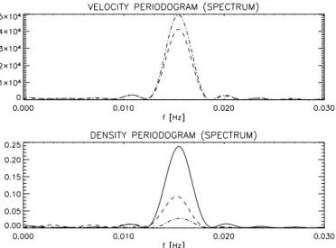
In Fig. 1 we present a periodogram (which here we use interchangeably with the (power) spectrum, although strictly speaking the power spectrum is a theoretical quantity defined as an integral over continuous time, and of which the peri-odogram is simply an estimate based on a finite amount of dis-crete data) of the velocity and density time series outputted at
Fig. 1.Case of apex (symmetric) heating: periodogram (spectrum) of the velocity and density oscillatory component times series outputted in the following three points: loop apex (solid curve), 1/4 (dash-dotted curve) and 1/6 (dashed curve) of the effective loop length (48 Mm), i.e. ats=0,−12,−16 Mm.
the three points: loop apex, 1/4 and 1/6 of the effective loop length (48 Mm), i.e. ats=0,−12,−16 Mm (cf. Scargle 1982, and his Eq. (10) in particular). The first two points are cho-sen to test whether the simple analytic solution for 1D stand-ing sound waves (see below) is relevant in this case. The third point (1/6) was chosen arbitrarily (any spatial point along the loop where density and velocity of the standing waves does not have a node would be equally acceptable). As expected for a 2nd spatial harmonic of a standing sound wave in the velocity periodogram there are two clearly defined peaks and the largest peak corresponds to 1/4 of the effective loop length, while the smaller peak corresponds to 1/6. Note that at the loop apex the periodogram gives 0 (solid line is too close to zero to be seen in the plot). The density periodogram shows the oppo-site behaviour to that of the velocity with the largest peak cor-responding to the loop apex, while 1/6 of the effective loop length corresponds to a smaller peak, and 1/4 is close to zero. The locations of the peaks are at about 0.0155 Hz i.e. the period of the oscillation is 64 s. The period of a 2nd spatial harmonic of a standing sound wave should be
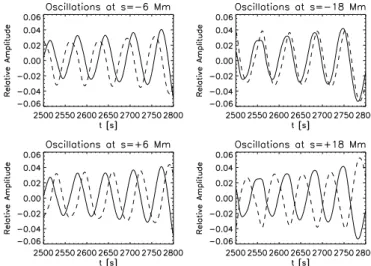
Fig. 2.Case of apex (symmetric) heating: oscillatory components of time series outputted at ±6 Mm and ±18 Mm in the time inter-val of 2500−2800 s. The solid curve shows plasma number density in units of 1011 cm−3. The dashed curve shows velocity normalized to 400 km s−1.
study the phase shift between the velocity and density oscilla-tions and compare our simulation results with analytic theory. In Fig. 2 we plot time series, outputted at±6 and±18 Mm, of the plasma number density in units of 1011cm−3and velocity, normalized to 400 km s−1. These points were selected so that one symmetric (with respect to the apex) pair (±6 Mm) is close to the apex, while another pair (±18 Mm) is closer to the foot-points. We choose these pairs because we wanted to compare how the phase shift is affected by spatial location. One would expect stronger upflows close to footpoints (due to chromo-spheric evaporation), which in turn alters the phase shift. Note that phase shift between the density and velocity is different (see below) for standing and propagating (with flows) acoustic waves). We gather from the graph that: (A) clear quasi-periodic oscillations are present; (B) they are shifted with respect to each other in time; (C) near the apex (±6 Mm) the phase shift is close to that predicted by 1D analytic theory; (D) close to the footpoints (±18 Mm) the phase shift is somewhat different from the one predicted by 1D analytic theory. In the last case the discrepancy can be attributed to the presence of flows near the footpoints. The main reason for the overall deviation is due to the fact that analytic theory does not take into account varia-tions of background density and velocity in time and that den-sity gradients in the transition region are not providing perfect reflecting boundary conditions for the formation of standing sound waves.
Another interesting result is that even with the wide variation of the parameter space of the flare, its duration, peak average temperature, etc., we always obtained a domi-nant 2nd spatial harmonic of a standing sound wave with some small admixture of 4th and sometimes 6th harmonics. Our ini-tial guess was that this is due to the symmetric excitation of these oscillations (recall that we use apex heat deposition). In order to investigate the issue of excitation further we decided to break the symmetry and put the heating source at one footpoint, hoping to see excitation of odd harmonics 1st, 3rd, etc.
Fig. 3.Case of single footpoint (asymmetric) heating: average temper-ature, temperature at apex, and number density at the apex as functions of time.
2.2. Case of single footpoint (asymmetric) heating
For single footpoint heating we fix s0 = 30 Mm in Eq. (1) in Nakariakov et al. (2004), i.e. (spatial) peak of the heating is chosen to be at the bottom of the transition region (top of chromosphere). Initially we run a code without flare heating, i.e. we putα = 0 (in this manner we turn offflare heating). E0=0.02 erg cm−3s−1was chosen such that in the steady (non-flaring) case the average loop temperature stays at about 1 MK. Then, we run the code with flare heating, i.e. we putα=1, and fixQp at 1×10⁴, so that it yields a peak average temperature of about 30 MK. The results are presented in Fig. 3. During the flare the apex temperature peaks at 38.38 MK while the num-ber density at the apex peaks at 3.11×1011cm−3. In this case, as opposed to the case of symmetric (apex) heating, the veloc-ity dynamics is quite different. Since the symmetry of heating is broken there is a non-zero net flow through the apex at all times. However, as in the symmetric heating case, we again see quasi-periodic oscillations superimposed on the dynamics of all physical quantities (cf. time interval oft = 2400−2700 in Fig. 3).
In Fig. 4 we present time-distance plots of velocity and den-sity for the time interval 2400−2700 s, where the quasi-periodic oscillations are most clearly seen. Here we again subtracted the slowly varying background (with respect to oscillation period). The picture is quite different from the case of apex (symmetric) heating (compare it with Fig. 2 in Nakariakov et al. 2004). This is because now the node in the velocity (at the apex) moves back and forth periodically along the apex, and at later times (t > 2550 s) stronger flows are now present. However, the physical nature of the oscillations remains mainly the same. i.e. a 2nd spatial harmonic of a sound wave, but now with an oscillating node at the apex.
354 D. Tsiklauri et al.: Flare generated acoustic oscillations
Fig. 4.Time-distance plots of the velocity and density oscillatory com-ponents in the time interval of 2400−2700 s for the case of single foot-point (asymmetric) heating.
in the case of apex (symmetric) heating. In the velocity peri-odogram at the apex there is a peak with a frequency higher than that of 2nd spatial harmonic of a standing sound wave. This is the frequency with which the node of the velocity oscil-lates (see discussion in the previous paragraph). It has nothing to do with the standing mode, but is dictated by the excitation conditions of the loop which acts as a dynamic resonator. Let us analyze now how this periodogram compares with 1D ana-lytic theory. The peak in the periodogram corresponding to 1/6 of the effective loop length (dashed line) corresponds to a fre-quency of about 0.017 Hz, i.e. the period of oscillation is 59 s. Again, the period of a 2nd spatial harmonic of a standing sound wave should be calculated from Eq. (3). If we substitute the ef-fective loop lengthL = 48 Mm (see Fig. 4) and an average temperature of 26 MK (see top panel in Fig. 3 in the range of 2400−2700 s) we obtain 62 s, which is close to the result of our numerical simulation (59 s).
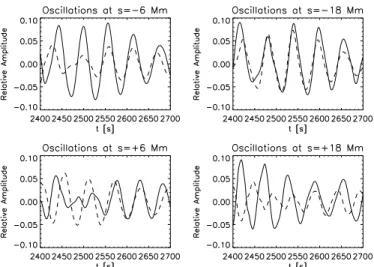
Next, we studied the phase shift between velocity and den-sity oscillations, and compare our simulation results with the 1D analytic theory. In Fig. 6 we produce a plot similar to Fig. 2, but for the case of asymmetric heating. The deviation, which is greater than in the case of apex (symmetric) heating, can again be attributed to the over-simplification of the 1D analytic theory, which does not take into account time variation of the background physical quantities and imperfection of the reflect-ing boundary conditions (see above). More importantly, in the asymmetric case strong flows are present throughout the flare simulation time. Thus, if linear time dependence is assumed, which is relevant within the short interval 2400−2700 s of the flare, then Eqs. (1) and (2) would be modified such that phase shifts would vary secularly in time. This is similar to that seen in Fig. 6.
Yet another interesting observation comes from the follow-ing argument: in a steady 1D case analytic theory predicts that the phase shift between the density and velocity should be (A) zero for for a propagating acoustic wave and (B) quar-ter of a period for the standing acoustic wave. Since in the
Fig. 5.As is Fig. 1 but for the case of single footpoint (asymmetric) heating. Time interval here is 2400−2700 s.
Fig. 6.As in Fig. 2, but for the case of single footpoint (asymmetric) heating. Time interval here is 2400−2700 s.
asymmetric case strong flows are present, we see less phase shift between the velocity and density in Fig. 6 as one would expect.
Thus, the results of the present study provide further, and more definitive proof than in Nakariakov et al. (2004) that these oscillations are indeed the 2nd spatial harmonic of a standing sound wave. However, the present work also reveals that in the case of single footpoint (asymmetric) heating the physical nature of the oscillations is more complex, as the node in the velocity oscillates along the apex and net flows are present.
3. Conclusions
As a byproduct of that study, in practically all the numeri-cal runs quasi-periodic oscillations in all physinumeri-cal quantities were detected (Nakariakov et al. 2004). Such oscillations are frequently seen during the solar flares observed in X-rays, 8−20 keV (e.g., Terekhov et al. 2002) as well as stellar flares observed in white-light (e.g., Mathioudakis et al. 2003). Our present analysis shows that quasi-periodic oscillations seen in our numerical simulations bear many similar features com-pared to observational datasets. In this work we tried to answer importantoutstanding questions(cf. Introduction section) that arose from the previous analysis (Nakariakov et al. 2004).
In summary the present study (and Nakariakov et al. 2004) established the following features:
– We show that the time dependences of density and tem-perature in a flaring loops contain well-pronounced quasi-harmonic oscillations associated with standing slow mag-netoacoustic modes of the loop.
– For a wide range of physical parameters, the dominant mode is the second spatial harmonic, with a velocity os-cillation node and the density osos-cillation maximum at the loop apex. This result is practically independent of the po-sitioning of the heat deposition in the loop.
– Because of the change of the background temperature and density, and the fact that density gradients in the transition region are not providing perfect reflecting boundary condi-tions for the formation of standing sound waves, the phase shift between the density and velocity perturbations is not exactly equal to a quarter of a period.
– We conclude that the oscillations in the white light, radio and X-ray light curves observed during solar and stellar flares may be produced by slow standing modes, with the period determined by the loop temperature and length. – For a typical solar flaring loop the period of oscillations
is shown to be about a few minutes, while amplitudes are typically of a few percent.
The novelty of this study is that by studying the spectrum and phase shift of these oscillations we provide more definite proof that these oscillations are indeed the 2nd harmonic of a stand-ing sound wave, and that the sstand-ingle footpoint (asymmetric) heat
positioning still produces 2nd spatial harmonics, although it is more complex than the apex (symmetric) heating as the node in the velocity oscillates along the apex and net flows are also present.
Acknowledgements. This research was supported in part by PPARC, UK. Numerical calculations of this work were performed using the PPARC funded MHD Cluster at St Andrews and Astro-Sun clus-ter at Warwick. D.T. would like to thank the referee, Dr. Mihalis Mathioudakis, for useful comments. D.T. kindly acknowledges sup-port from Nuffield Foundation through an award to newly appointed lecturers in science, engineering and mathematics (NUF-NAL 04).
References
Arber, T. D., Longbottom, A. W., Gerrard, C. L., & Milne, A. M. 2001, J. Comput. Phys., 171, 151
Aschwanden, M. J. 1987, Sol. Phys., 111, 113
Aschwanden, M. J., & Alexander, D. 2001, Sol. Phys., 204, 93 Aschwanden, M. J., Brown, J. C., & Kontar, E. P. 2002, Sol. Phys.,
210, 383
Mathioudakis, M., Seiradakis, J. H., Williams, D. R., et al. 2003, A&A, 403, 1101
McKenzie, D. E., & Mullan, D. J. 1997, Sol. Phys., 176, 127 Nakariakov, V. M., Tsiklauri, D., Kelly, A., Arber, T. D., &
Aschwanden, M. J. 2004, A&A, 414, L25
Ofman, L., Nakariakov, V. M., & DeForest, C. E. 1999, ApJ, 514, 441 Ofman, L., & Wang, T. J. 2002, ApJ, 580, L85
Peres, G., Rosner, R., Serio, S., & Vaiana, G. S. 1982, ApJ, 252, 791 Priest, E. R. 1982, Solar Magnetohydrodynamics (Holland,
Dordrecht: D. Reidel Publ. Comp.)
Rosner, R., Tucker, W. H., & Vaiana, G. S. 1978, ApJ, 220, 643 Scargle, J. 1982, ApJ, 263, 835
Terekhov, O. V., Shevchenko, A. V., Kuz’min, A. G., et al. 2002, Astron. Lett., 28, 397
Tsiklauri, D., Aschwanden, M. J., Nakariakov, V. M., & Arber, T. D. 2004, A&A, 419, 1149
Wang, T., Solanki, S. K., Curdt, W., Innes, D. E., & Dammasch, I. E. 2002, ApJ, 574, L101