WORKING PAPERS SERIES
WP04-06
Testing and Modelling Market Microstructure
Effects with an Application to the Dow Jones
Industrial Average
Testing and Modelling Market Microstructure E
ff
ects with an
Application to the Dow Jones Industrial Average
∗Basel Awartani†
Queen Mary, University of London
Valentina Corradi‡
Queen Mary, University of London
Walter Distaso§ University of Exeter
January 2004
Preliminary and incomplete
Abstract
It is a well accepted fact that stock returns data are often contaminated by market microstructure effects, such as bid-ask spreads, liquidity ratios, turnover, and asymmetric information. This is particularly relevant when dealing with high frequency data, which are often used to compute model free measures of volatility, such as realized volatility. In this paper we suggest two test statistics. The first is used to test for the null hypothesis of no microstructure noise. If the null is rejected, we proceed to perform a test for the hypothesis that the microstructure noise variance is independent of the sampling frequency at which data are recorded. We provide empirical evidence based on the stocks included in the Dow Jones Industrial Average, for the period 1997-2002. Our findings suggest that, while the presence of microstructure induces a severe bias when estimating volatility using high frequency data, such a bias grows less than linearly in the number of intraday observations.
Keywords: Bipower variation, market microstructure, Realized Volatility. JEL classification: C22, C12, G12.
∗The authors gratefully acknowledge financial support from the ESRC, grant code R000230006.
†Queen Mary, University of London, Department of Economics, Mile End, London, E14NS, UK, email: [email protected].
‡Queen Mary, University of London, Department of Economics, Mile End, London, E14NS, UK, email: [email protected].
1
Introduction
Dating back to Black’s (1986) seminal paper, it is a well accepted fact that transaction data occurring in financial markets are often contaminated by market microstructure effects, such as bid-ask spreads, liquidity ratios, turnover, and asymmetric information (see also e.g. Hasbrouk (1993), Bai, Russell and Tiao (2000), Hasbrouck and Seppi (2001), O’Hara (2003) and references therein). It is argued in these papers that the observed transaction price can be decomposed into the efficient one plus a “noise” due to microstructure effects.
This fact is particularly relevant when dealing with high frequency data, which are often used to compute model free measures of volatility, such as realized volatility (see e.g. Barndorff-Nielsen and Shephard (2002, 2003, 2004c), Andersen, Bollerslev, Diebold and Labys (2001, 2003), Meddahi (2002) and Andersen, Bollerslev and Meddahi (2004)) and bipower variation (Barndorff-Nielsen and Shephard, 2004a,b). Although the relevant limit theory suggests that volatility estimates get more precise as the frequency of observations increases, this is not necessarily valid in the presence of microstructure noise which is not accounted for. The effect of microstructure noise on high frequency volatility estimators has been recently analyzed by A¨ıt-Sahalia, Mykland and Zhang (2003), Zhang, Mykland and A¨ıt-Sahalia (2003), and Bandi and Russell (2003a,b). These papers point out that changes in transaction prices over very small time intervals are mainly composed of noise and carry little information about the underlying return volatility. This is because, at least for the class of continuous semimartingale processes, volatility is of the same order of magnitude as the time interval, while the microstructure noise has a roughly constant variability. Therefore, as the time interval shrinks to zero, the signal to noise ratio related to the observed transaction prices also tends to zero, and using the estimators of volatility mentioned above one may run the risk of estimating the variance of the microstructure noise, rather than the underlying return volatility.
Hence, the need of measures of return volatility which are robust to the presence of market microstructure effects. An important contribution in this direction is that of Zhang, Mykland and A¨ıt-Sahalia (2003), who suggest an asymptotically unbiased volatility estimator, based on subsam-pling techniques. The validity of their estimator hinges on the chosen model for the microstructure noise.
and rare jumps. Second, if the null is rejected, we test the null hypothesis of correct specification of the model of microstructure noise of A¨ıt-Sahalia and Mykland and Zhang (2003), which assumes that the microstructure noise has a constant variance, regardless of the frequency at which data are sampled.
The first test statistic is based on the difference between two realized volatilities computed at different sampling intervals, say one minute and ten minutes. Under the null, both estimators will converge to the true integrated volatility process, though at a different speed. Given this, by properly scaling this difference we have a statistic with a normal limiting distribution under the null and unit asymptotic power. However, such a test statistic can diverge because of the presence of either microstructure noise or jumps. To overcome this problem, we also provide a jump robust version of the test, which is based on recent results by Barndorff-Nielsen and Shephard (2004a,b) and Corradi and Distaso (2004).
The second test statistic is based on the difference between two estimators of the microstructure noise computed again over different time intervals. Under the null model of a noise with constant variance, by properly scaling this difference we obtain a statistic with a normal limiting distribution. The test is consistent against the alternative of a noise with variance depending on the chosen sampling frequency. Indeed, an alternative model of economic interest would be one in which the microstructure noise variance is positively correlated with the time interval.
The proposed tests are then applied to transaction data recorded for the stocks included in the Dow Jones Industrial Average (DJIA) for the period 1997-2002, using a fixed time span equal to five days. The tests are computed over the different five days intervals. The empirical analysis suggests that while the presence of microstructure effects induces a severe bias when estimating volatility using high frequency data, such a bias grows less than linearly in the number of intraday observations.
2
Methodology
2.1 Set-up
Let Xt = log(St), where St denotes the price of a financial asset or derivative. Throughout the
paper it is assumed thatXt follows a process of the type
Xt=µtdt+ctdqt+σtdWt, (1)
where Wt is a standard Brownian motion. As for the jump component, Pr(dqt = 1) = λtdt,
where λt is independent of σt2, ct is an i.i.d. process and is assumed to be independent of dqt.
This specification of the jump component covers the case of large and rare jumps, analyzed by Barndorff-Nielsen and Shephard (2004a). Although we cannot observe the trajectory ofXt, we still
have data recorded at high frequency. Suppose that the number of daily observations is denoted by T and that, for each day, we have M intraday observations; therefore, over a fixed time span,
sayT , we have a total ofT M observations. Realized volatility is defined as
RVt,T ,M =
T M
!
i=1
" Xt+ i
M −Xt+
i−1 M
#2
, 0≤t≤T −T .
If Xt belongs to the class of continuous semimartingales (if dqt = 0, a.s., ∀ t, i.e. there are no
jumps in the log price process), then (see e.g. Karatzas and Shreve (1991), Ch.1), asM → ∞,
RVt,T ,M →Pr $ t+T
t
σs2ds=IVt,T. (2)
Here σs2 denotes the instantaneous volatility at times, that is
lim
h→0
E"(Xs+h−Xs)2|'s
#
h =σ
2
s,
where's refers to the relevant conditioning set at times.
However, if Xt is the sum of a continuous semimartingale component and a jump component,
then the statement in (2) does no longer hold and, as pointed out by Barndorff-Nielsen and Shephard (2004a),
RVt,T ,M →PrIVt+ Nt+T
!
i=Nt
whereNtis a counting process andcidenotes the size of the jumps. Interestingly, Barndorff-Nielsen
and Shephard (2004a) also suggest a measure of integrated volatility, namely bipower variation, which (when properly scaled) is a consistent estimator of integrated volatility and is robust to the presence of rare of large jumps.1 Bipower variation is defined as
BVt,T ,M =
T M!−1
i=1
% % %Xt+i+1
M −Xt+
i M % % % % % %Xt+i
M −Xt+
i−1 M
% %
%, 0≤t≤T −T .
Now, suppose that we can observeSt+ i
M only up to an error, so that the observed price process is given by
& St+i
M =St+Mi ηt+Mi , t= 0,1, . . . , T −1. (4) Therefore
logS&t+ i
M = logSt+Mi + logηt+Mi , or (5)
Yt+ i
M = Xt+Mi +$t+Mi . Here $t+ i
M is interpreted as a noise capturing the market microstructure effect. Similarly to what is customarily assumed in the literature,Xt+i/M and $t+i/M are independent andE'$t+i/M( = 0.
Now,
E"Yt+ i
M−Yt+iM−1
#2
= E"Xt+ i
M−X
i−1 M
#2
+E"$t+ i M−$t+
i−1 M
#2
+E"$t+i M−$t+
i−1 M
# " Xt+ i
M−Xt+
i−1 M
#
= E"Xt+ i
M−X
i−1 M
#2
+E"$t+ i M−$t+
i−1 M
#2
. (6)
In the case of Xt being a continuous semimartingale, E
" Xt+i
M −Xt+i−M1
#2
=O(M−1). Also, we
will assume that
lim
M,N→∞, N/M→0
E )
*T M−1
i=1
"
$t+ i M −$t+
i−1 M
#2+
N =∞.
As for bipower variation, note that, by Minkowski inequality,
E
T M!−1
i=1
% % %Yt+i+1
M −Yt+
i M % % % % % %Yt+ i
M −Yt+
i−1 M
% % %
≤E
T M!−1
i=1
% % %Xt+i+1
M −Xt+
i M % % % % % %Xt+i
M −Xt+
i−1 M % % %
+E
T M!−1
i=1
% % %$t+i+1
M −$t+Mi
% % %%%%$t+i
M −$t+i−M1
% % %
+E
T M!−1
i=1
% % %$t+i+1
M −$t+Mi
% % %%%%Xt+i
M −Xt+i−M1
% % %
.
Therefore, when using bipower variation it is not immediate how to decompose the total variability in integrated volatility and noise variance. Nevertheless, it is evident that, while bipower variation is robust to the presence of the jump component, it is not robust to microstructure effects.
As mentioned in the Introduction, our objective is perform a test for the null hypothesis of no microstructure effects over a sequence of finite time span (e.g. 5 working days) periods, and, for the cases in which the null is rejected, proceed to test the null hypothesis that the microstructure noise has constant variance, regardless of the sampling interval over which we compute realized volatility.
2.2 Testing the null hypothesis of no microstructure effects
In the sequel we shall assume that the true asset price process is generated as in (1). Define the following hypotheses:
H0 :E
"
$t+i
M −$t+
i−1 M
#2
= 0, for all M, t (7)
and
HA:E
"
$t+i
M −$t+i−M1
#2
(
= 0, (8)
whereE'$t+i/M −$t+(i−1)/M(2 and $t+i/M are defined respectively in (6) and (5).
Therefore the null hypothesis implies that there are no microstructure effects in the observed transaction prices, while the alternative is simply the negation of the null.
In order to test H0 versusHA,we propose the following statistic
ZM,N,T ,t= √
N T )
*T M i=1
" Yt+i
M −Yt+
i−1 M
#2
−*T Ni=1
" Yt+i
N −Yt+
i−1 N
#2+
0
2 3N T
*N T i=1
" Yt+i
N −Yt+
i−1 N
#4 , (9)
where N/M → 0 as M, N → ∞ (i.e. M grows faster than N). The numerator in (9) can be
expanded as
1
N T (10)
× T M ! i=1 " Yt+i
M −Yt+
i−1 M
#2
−
$ t+T
t
σ2sds − T N ! i=1 " Yt+i
N −Yt+
i−1 N
#2
−
$ t+T
t
σ2sds
Inspection of (10) reveals the logic behind the choice of the test statistic in (9); if there are no mi-crostructure effects (under the maintained assumption of no jumps), then both*T M
i=1
'
Yt+i/M −Yt+(i−1)/M(2
and*T N i=1
'
Yt+i/N −Yt+(i−1)/N
(2converge in probability to the true integrated volatility,2t+T t σ2sds.
Also, by the central limit theorems in Barndorff-Nielsen and Shephard (2002 and 2004c),
T M ! i=1 " Yt+ i
M −Yt+
i−1 M
#2
−
$ t+T
t
σs2ds
=Op(M−1/2)
and T N ! i=1 " Yt+i
N −Yt+
i−1 N
#2
−
$ t+T
t
σs2ds
=Op(N−1/2).
Therefore, under the null hypothesis, provided that asN, M → ∞,N/M →0, 1 N T T M ! i=1 " Yt+i
M −Yt+i−M1
#2
−
$ t+T
t
σ2sds
=op(1).
Under H0, the limiting distribution of the test statistic is driven by
− √
N T )
*T N i=1
" Yt+i
N −Yt+
i−1 N
#2
−2tt+T σ2sds
+
0
2 3N T
*N T i=1
" Yt+i
N −Yt+i−N1
#4 ,
which is asymptotically standard normal. Under the alternative, we expect*T M i=1
'
Yt+i/M −Yt+(i−1)/M
(2
to be of a larger order of magnitude (in probability) than*T N i=1
'
Yt+i/N −Yt+(i−1)/N(2, and so we
expect the statistic to diverge.
A possible problem with the statistic above is that standard normal critical values are no longer correct in the presence of jumps. In fact, in the presence of jumps, the numerator of (9) has a non zero mean and the square of the denominator is not a consistent estimator for the true integrated quarticity (i.e. 2t+T
t σs4ds).Therefore, we also suggest a statistic which is robust to jumps
ZBM,N,T ,t= µ
−2 1
√ N T 3
2.6090µ−14
(11)
×
"*T M−1
i=1
% % %Yt+i+1
M −Yt+
i M
% % %%%%Yt+ i
M−Yt+iM−1
% %
%−*T Ni=1
% % %Yt+i+1
N −Yt+
i N
% % %%%%Yt+i
N−Yt+i−N1
% % %# 0
N T*T Mi=1−3%%%Yt+i+4
M −Yt+
i+3 M % % % % % %Yt+i+3
M −Yt+
i+2 M % % % % % %Yt+i+2
N −Yt+
i+1 N % % % % % %Yt+i+1
N −Yt+
i N % % % ,
where µ1 = E(|N(0,1)|). Under the null hypothesis, the statistic above has a standard normal
2.3 A simple specification test for the microstructure noise
For all the periods in which, according to either or both test statistics proposed in the previous subsection, we reject the null hypothesis of no microstructure noise, it may be interesting to perform a specification test for the microstructure error. In particular, the hypothesis of interest is that of the microstructure noise having a constant variance, independent of the frequency at which data are recorded. In fact, most of the recent literature on incorporating microstructure effects (see e.g. A¨ıt-Sahalia, Mykland and Zhang (2003), Zhang, Mykland and A¨ıt-Sahalia (2003), and Bandi and Russell (2003a,b)) postulates a model of noise with constant variance.
More precisely, letE'$t+i/M −$t+(i−1)/M(2= 2νt,M andE'$t+i/M −$t+(i−1)/M
(2 = 2
νt,N. The
null and alternative hypotheses can be formulated as follows
H0$ :νt,M =νt,N, for all M, N (12)
and
HA$ :νt,M <νt,N. (13)
Thus, the alternative of interest is that the variance of the microstructure noise is negatively correlated with the frequency at which data are recorded. The alternative hypothesis is compatible with the microstructure noise model outlined by Barndorff-Nielsen and Shephard (2004b), who specify a two component model; the first is a jump component and the second is an error process with the variance decaying to zero at a rate 1/√M. As a consequence, the bias incurred in
estimating volatility using realized volatility grows less than linearly in the number of intraday observations.2 We propose the following test statistic
VM,N,T ,t=1N T
*T M i=1 )
Yt+ i
M−Yt+iM−1 +2
2T M −
*T N i=1 )
Yt+i
N−Yt+i−N1 +2
2T N
0
1
N T
*N T i=1
" Yt+i
N −Yt+i−N1
#4
. (14)
The logic behind the statistic proposed above is the following. Under the null hypothesis, both
*T M i=1
'
Yt+i/M −Yt+(i−1)/M(2/2T M and *iT N=1'Yt+i/N −Yt+(i−1)/N(2/2T N converge to the same
probability limit, say ν, though the former converges faster than the latter. Thus,
1 N T
*T M i=1 )
Yt+i
M−Yt+i−M1 +2
2T M −ν
0
1
N T
*N T i=1
" Yt+i
N −Yt+
i−1 N
#4
is asymptotically negligible and the statistic in (14) is asymptotic equivalent to
−1N T
*T N i=1 )
Yt+i
N−Yt+i−N1 +2
2T N −ν
0
1
N T
*N T i=1
" Yt+i
N −Yt+i−N1
#4
,
which has a standard normal limiting distribution (see Theorem A1 in Zhang, Mykland and A¨ıt-Sahalia (2003)).
Under the alternative,*T M i=1
'
Yt+i/M −Yt+(i−1)/M(2/2T M and*iT N=1'Yt+i/N −Yt+(i−1)/N(2/2T N
converge respectively toνM and νN, and thus the statistic diverges.
In the next subsection, the limiting distributions of the proposed test statistics are derived.
2.4 Main theoretical results
In the sequel we need the following assumptions A1: Xt is generated as in (1).
A2: 2t+T
t σ4(s)ds <∞,almost surely, for anytand T.
A3: E"$i
M −$
i−1 M
#4
<∞.
A4: *M T i=1
'
$t+i/M −$t+(i−1)/M
(2
/M T =op(b−t,M1 ),and*iN T=1'$t+i/N −$t+(i−1)/N
(2
/N T =op(b−t,N1),
where, as M, N → ∞, bt,M
bt,NM
1−α → ∞,forα∈(0,1) andN =Mα. A4’: E"*M Ti=1 '$t+i/M −$t+(i−1)/M
(2
/M T#= νt,M and E"*N Ti=1'$t+i/N −$t+(i−1)/N
(2
/N T#=
νt,N,
√
N(νt,M/νt,N)→ ∞,asM, N → ∞.
Notice thatA1and A2 are customary in the literature on realized volatility;A3requires a finite fourth moment of the market microstructure noise and seems to be trivially satisfied. Finally, A4 allows the variability of the microstructure error to decrease with the sampling interval. In particular, the variance of the microstructure noise is allowed to approach zero as the sampling interval goes to zero, but at a slow enough rate.
Proposition 1
(i) Let A1-A2 hold and assume that λt = 0 for all t. Under H0, defined in (7), as M, N → ∞
and N/M →0,
ZM,N,T ,t→d N(0,1).
(ii) Let A1-A4 hold. UnderHA,defined in (8), as M → ∞, for ε>0,
lim
M→∞Pr
) bt,N
bt,M
Mα−1ZM,N,T ,t>ε
+
= 1.
Therefore, we can just perform a one-sided test and reject the null hypothesis of no microstructure effects when we get a value forZM,N,T ,t larger than, say, the 95% percentile of a standard normal.
In the proposition above, the statement under the null is robust to possible leverage effects, but not to possible jumps.
The null limiting distribution and power properties of the jump robust version of the test for no microstructure effects test are given in the next Proposition.
Proposition 2
(i) Let A1-A2 hold and assume that µt = 0 for all t and that σt in (1) is independent of Xt.
Under H0,defined in (7), as M, N → ∞ andN/M →0,
ZBM,N,T ,t→d N(0,1).
(ii) Let A1-A4 hold. UnderHA,defined in (8), as M → ∞, for ε>0,
lim
M→∞Pr
) bt,N
bt,M
Mα−1ZBM,N,T ,t>ε
+
= 1.
As outlined in the previous subsection, every time we reject the null hypothesis in (7), according to either or both the suggested statistics, we may be interested in performing a specification test for the microstructure noise. Its properties are given in the next Proposition.
Proposition 3
(i) Let A1-A3 hold. UnderH0$,defined in (12), asM, N → ∞, N/M →0,
(ii) Let A1-A3 hold. Also, assume that
E 1
M T
M T
!
i=1
"
$t+i
M −$t+iM−1
#2
= 2νt,M and E
1
N T
N T
!
i=1
"
$t+i
N −$t+i−N1
#2
= 2νt,N
are such that √Mνt,M → ∞ and
√
Nνt,N → ∞.Under HA,defined in (13), as M → ∞, for
ε>0,
lim
M→∞Pr
) 1
√
N TVM,N,T ,t>ε +
= 1.
An application of the testing procedure outlined in this section to the stocks included in the Dow Jones Industrial Average is given in the next Section.
3
Empirical evidence from the Dow Jones Industrial Average
3.1 Data description
The empirical analysis of market microstructure effects is based on data retrieved from the Trade and Quotation (TAQ) database at the New York Stock Exchange. The TAQ database contains intraday trades and quotes for all securities listed on the New York Stock Exchange (NYSE), the American Stock Exchange (AMEX) and the Nasdaq National Market System (NMS). The data is published monthly on CD-ROM since 1993 and on DVD since June 2002. Our sample contains the DJIA stocks (30 stocks in total3) and extends from January 1, 1997 until December 24, 2002, for
a total of 1505 trading days.4 Also, in our empirical exampleT = 5 and therefore we have a total
of 301 five-days periods.
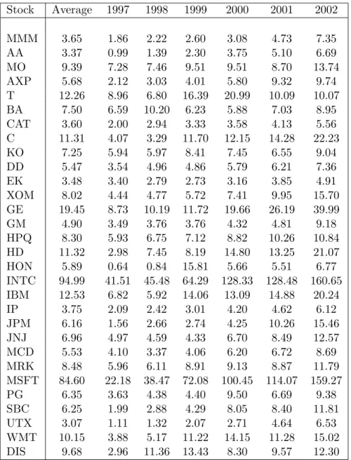
Table 2 shows the average number of quotations per minute for all individual stocks. The table presents a spectrum of liquidity, ranging from as low as 3 quotations per minute for United Technologies Corp. (UTX) to as high as 94 for Intel Corp.. The two most liquid stocks in the sample
3It is worth mentioning that the 30 companies included in the DJIA are not the same throughout the sample period. Woolworth, Bethlehem Steel, Texaco and CBS (Westinghouse Electric) have been replaced by Wal-Mart, Johnson & Johnson, Hewlett-Packard and Citigroup (Travelers Group) in 1997. In addition SBC Communications, Microsoft, Intel and Home Depot have replaced Union Carbide, Chevron, Goodyear, and Sears in 1999. Our sample contains the DJIA of individual firms as it was in 2000. The names and the symbols of the stocks included in the sample are reported in Table 1.
are Intel and Microsoft and it takes only a fraction of a second to have a fresh quote. Liquidity has increased substantially during the sample period and, as we approach 2002, the number of quotations per minute almost doubles for some stocks (e.g. 3M Company (MMM), Citigroup Inc. (C), Home Depot Corp. (HD), Microsoft (MSFT)).
From the original data set, which includes prices recorded for every trade, we extracted 1 minute and 10 minutes interval data, similarly to Andersen and Bollerslev (1997). Provided that there is sufficient liquidity in the market, the 5 minutes frequency is generally accepted as the highest frequency at which the effect of microstructure biases are not too distorting (see Andersen, Bollerslev, Diebold and Labys (2001), Andersen, Bollerslev and Lang (1999) and Ebens (1999)); hence the choice of the two mentioned frequencies to calculate the test statistics, in order to highlight the full extent of the microstructure noise effects.
The price figures for each 1 and 10 minutes intervals are determined as the interpolated average between the preceding and the immediately following quotes, weighted linearly by their inverse relative distance to the required point in time. For example, suppose that the price at 15:29:56 was 11.75 and the next quote at 15:30:02 was 11.80, then the interpolated price at 15:30:00 would be exp(1/3×log(11.80) + 2/3×log(11.75)) = 11.766. From the 1 and 10 minutes price series
we calculated 1 and 10 minutes intradaily returns as the difference between successive log prices expressed in percentages; then
Rt+i
N = 100×
"
log(Yt+i
N)−log(Yt+i−N1)
# ,
where Rt+i/N denotes the return for intraday periodi/N on trading dayt, witht = 0, . . . , T−1.
The New York Stock Exchange opens at 9:30 a.m. and closes at 4.00 p.m.. Therefore a full trading day consists of 391 (resp. 40) intraday returns calculated over an interval of one minute (resp. ten minutes). For some stocks, and in some days, quotations arrive some time after 9:30; in these cases we always set the first available trading price after 9:30 a.m to be the price at 9:30 a.m.. Not all the days in our sample consists of 391 (resp. 40) price observations; this is attributable to the fact that the NYSE closes early on certain days, such as on Christmas Eve5; for all these intervals
without price quotes we insert zero return values. Highly liquid stocks may have more than one price at certain points in time (for example 5 or 10 quotations at the same time stamp is normal
for INTC and MSFT); when there exists more than one price at the required interval, we select the last provided quotation. For interpolating a price from a multiple price neighborhood, we select the closest provided price for the computation.
3.2 Testing for the null of no microstructure effects
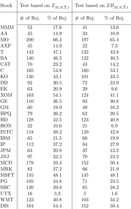
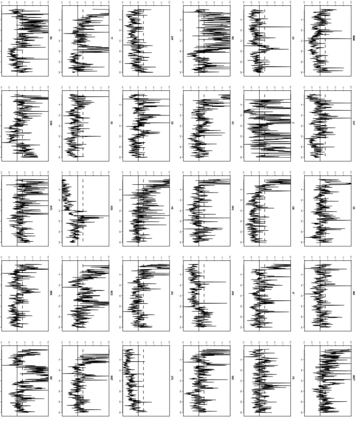
Table 3, columns 2 and 3, reports the findings for the test based on the statistic defined in (9). More precisely, we report the number and the percentages of rejections, based on a one-sided test. We first notice that only for six stocks the percentage of rejection is below 20% of the cases. For twelve stocks the percentage of rejection is between 20% and 40% of the cases, and for the remaining twelve stocks it is higher than 40% with a maximum of 66%.This indicates that, though
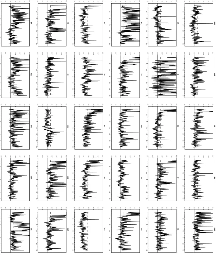
microstructure effect plays an important role, its contribution is quite variable over time. Overall, we do not find evidence of a clear relationship between liquidity and microstructure effects. For example, taking two rather liquid stocks like IBM and Intel, for the former we reject the null about 20% of the times, while for the latter we reject about 39% of the times. In Figure 1, we report the plot of the test statistic over the different 5 days intervals considered, with the dotted line representing the 5% upper tail critical value of a standard normal. We notice that there are a few instances in which the statistic takes a large and negative values. This happens mainly for stocks characterized by low liquidity, such as EK and HON. The reason for this finding is that, since these stocks are not very liquid, and therefore are not traded often enough, a lot of returns over 1 minute interval are zero, while are not zero over 10 minutes interval. Hence a negative value for the test statistic.
noise effect, we perform a specification test for the hypothesis of a microstructure noise with constant variance (independent of the sampling interval). The relevant empirical results are contained in the next subsection.
3.3 A specification test for the variability of the microstructure noise
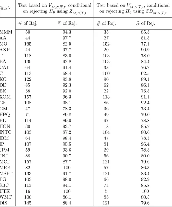
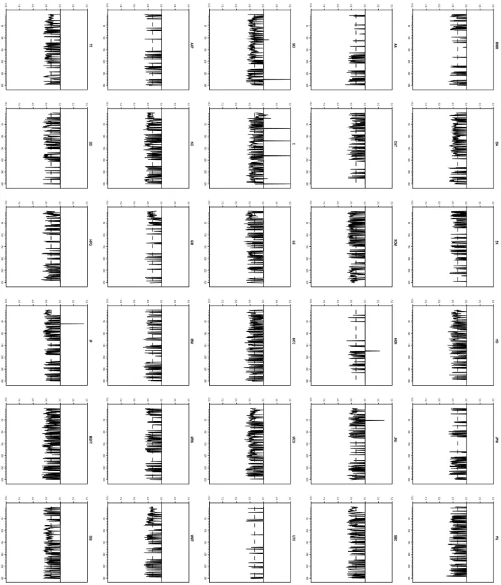
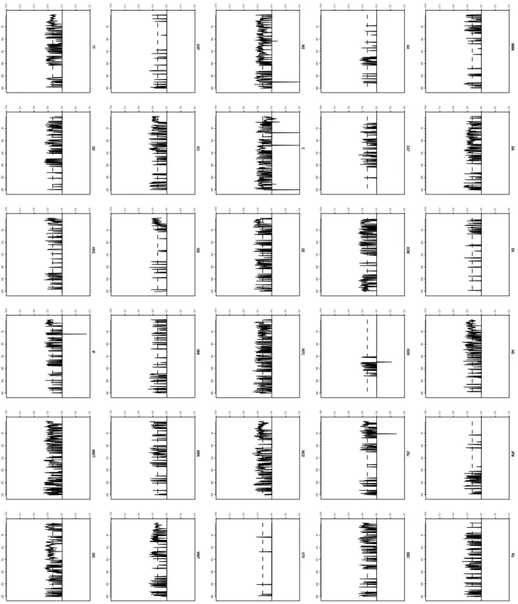
For all the periods in which we reject the null hypothesis of no market microstructure effects, we then testH0$ versusHA$ ,defined respectively in (12) and (13), using the statistic suggested in (14).
We perform two sequences of test, the first one conditional on rejecting the null of no microstructure using the test statistic in (9) and the second conditional on the same outcome using the statistic in (11). The results are reported in Table 4, columns 2 to 5, and the plots are given in Figures 3 and 4. It is immediate to see that the null hypothesis is rejected in almost all the cases. This provides strong evidence that while the presence of microstructure induces a severe bias when estimating volatility using high frequency data, such a bias grows less than linearly in the number of intraday observations. In fact, given (6), acceptance of the null hypothesis would imply that
E 6M
!
i=1
" Yt+i
M −Yt+
i−1 M
#27
= E 6M
!
i=1
" Xt+ i
M −Xt+
i−1 M
#27
+E 6M
!
i=1
"
$t+ i M −$t+
i−1 M
#27
,
$ t+1
t
σs2ds+ 2MνM =
$ t+1
t
σs2ds+ 2Mν.
However, our findings strongly suggest thatνM <νN,thus indicating that the microstructure bias
grows at a slower than linear rate as the number of intraday observations increases.
4
Concluding remarks
References
A¨ıt-Sahalia, Y. (2004), Disentangling Diffusion from Jumps,Journal of Financial Economics, forthcom-ing.
A¨ıt-Sahalia, Y., P.A. Mykland and L. Zhang (2003), How Often to Sample a Continuous Time Process in the Presence of Market Microstructure Noise, Working Paper, Princeton University.
Andersen, T.G., and T. Bollerslev, (1997) Intraday Periodicity and Volatility Persistence in Financial Markets, Journal of Empirical Finance, 4, 115-158.
Andersen, T.G., T. Bollerslev, F.X. Diebold and P. Labys, (2001) The Distribution of Realized Exchange Rate Volatility,Journal of the American Statistical Association, 96, 42-55.
Andersen, T.G., T. Bollerslev, F.X. Diebold and P. Labys, (2003) Modelling and Forecasting Realized Volatility, Econometrica, 71, 579-625.
Andersen, T.G., T. Bollerslev and F.X. Diebold (2003), Some Like it Smooth and Some Like it Rough: Untangling Continuous and Jump Components in Measuring, Modelling and Forecasting Asset Return Volatility, Working Paper, Duke University.
Andersen, T.G., T. Bollerslev and S. Lang (1999), Forecasting Financial Market Volatility. Sample Frequency vs Forecast Horizon,Journal of Empirical Finance, 6, 457-477.
Andersen, T.G., T. Bollerslev and N. Meddahi (2004), Analytic Evaluation of Volatility Forecasts, In-ternational Economic Review, forthcoming.
Bai, X., J.R. Russell and G. Tiao (2000), Effects on Nonnormality and Dependence on the Precision of Variance Estimates Using High Frequency Data, Working Paper, University of Chicago, Graduate School of Business.
Bandi, F.M., and J.R. Russell (2003a), Microstructure Noise, Realized Volatility, and Optimal Sampling, Working Paper, University of Chicago, Graduate School of Business.
Bandi, F.M., and J.R. Russell (2003b), Volatility or Noise? Working Paper, University of Chicago, Graduate School of Business.
Barndorff-Nielsen, O.E., and N. Shephard (2002), Econometric Analysis of Realized Volatility and Its Use in Estimating Stochastic Volatility Models,Journal of the Royal Statistical Society, Series B, 64, 253-280.
Barndorff-Nielsen, O.E., and N. Shephard (2003), Realized Power Variation and Stochastic Volatility, Bernoulli, 9, 243-265.
Barndorff-Nielsen, O.E., and N. Shephard (2004b), Econometrics of Testing for Jumps in Financial Economics Using Bipower Variation, Working Paper, University of Oxford.
Barndorff-Nielsen, O.E., and N. Shephard (2004c), A Feasible Central Limit Theory for Realized Volatil-ity under Leverage, Working Paper, UniversVolatil-ity of Oxford.
Black, F. (1986), Noise, Journal of Finance, XLI, 529-543.
Corradi, V., and W. Distaso (2004), Specification Tests for Daily Integrated Volatility, in the Presence of Possible Jumps, Working Paper, Queen Mary, University of London.
Ebens, H. (1999), Realized Stock Volatility, Working Paper, John Hopkins University.
Hasbrouck, J. (1993), Assessing the Quality of a Security Market. A New Approach to Transaction Cost Measurement, Review of Financial Studies, 6, 191-212.
Hasbrouck, J., and D. Seppi (2001), Common Factors in Prices, Order Flows, and Liquidity,Journal of Financial Economics, 59, 383-411.
Huang, X., and G. Tauchen (2003), The Relative Contribution of Jumps to Total Price Variation, Working Paper, Duke University.
Karatzsas, I., and S.E. Shreve (1991), Brownian Motion and Stochastic Calculus, Springer and Verlag, New York.
Meddahi, N. (2002), A Theoretical Comparison between Integrated and Realized Volatility,Journal of Applied Econometrics, 17, 475-508.
O’Hara, M. (2003), Presidential Address: Liquidity and Price Discovery, Journal of Finance, LVIII, 1335-1354.
Appendix
Proof of Proposition 1.
(i) The statistic defined in (9) can be expanded into
ZM,N,T ,t = 0 N M √ M T )* T M i=1 " Yt+ i
M −Yt+iM−1
#2
−2tt+Tσ2sds
+
0
2 3N T
*N T i=1
" Yt+i
N −Yt+
i−1 N #4 − √ N T )
*T N i=1
" Yt+i
N −Yt+
i−1 N
#2
−2tt+T σ2sds +
0
2 3N T
*N T i=1
" Yt+i
N −Yt+
i−1 N
#4 . (15)
Theorems 1 in Barndorff-Nielsen and Shephard (2002, 2004c) establish that, asM → ∞, 1
M T 6
RVt,T ,M,T−
$ t+T
t
σ2sds 7
d
→N 6
0,2 $ t+T
t
σ4sds 7
.
Therefore the first term in (15) isop(1), given that, asM, N → ∞,N/M →0. As a consequence,
the limiting distribution ofZM,N,T ,tunderH0 will be determined by the second component of (15).
By a similar argument as before, since, asN → ∞,
1 3N T
N T
!
i=1
" Yt+i
N −Yt+
i−1 N
#4 Pr
→
$ t+T
t
σs4ds,
the statement follows immediately.
(ii) Under the alternative hypothesis, it is possible to expand the numerators of the components of (15) respectively as
1 N T T M ! i=1 )" Xt+i
M −Xt+
i−1 M
#2
+"$t+i M −$t+
i−1 M
#2
+ 2"Xt+i
M −Xt+
i−1 M
# "
$t+ i M −$t+
i−1 M
#+
−
$ t+T
t
σ2sds :
and
−1N T T N ! i=1 )" Xt+i
N −Xt+i−N1
#2
+"$t+i
N −$t+i−N1
#2
+ 2"Xt+i
N −Xt+i−N1
# "
$t+i
N −$t+i−N1
−
$ t+T
t
σ2sds : . Similarly N T ! i=1 " Yt+i
N −Yt+i−N1
#4 = N T ! i=1 ;" Xt+i
N −Xt+
i−1 N
#4
+"$t+i N −$t+
i−1 N
#4
+ 6"Xt+i
N −Xt+
i−1 N
#2" $t+i
N −$t+ i−1
N
#2
+4"Xt+i
N −Xt+
i−1 N
#3" $t+i
N −$t+ i−1
N
#
+ 4"Xt+i
N −Xt+
i−1 N
# "
$t+i N −$t+
i−1 N
#3<
.
Therefore the statistic will diverge to plus infinity and the test will be consistent if, asN, M → ∞,
*T M i=1
"
$t+i
M −$t+
i−1 M
#2
−*T Ni=1
"
$t+i N −$t+
i−1 N
#2
0 *N T
i=1
"
$t+i N −$t+
i−1 N
#4 → ∞,
which holds under Assumption A4. !
Proof of Proposition 2. From Barndorff-Nielsen and Shephard (2004a), under the null hypoth-esis, as M → ∞,
T M!−1
i=1
µ−12%%%Yt+i+1
M −Yt+
i M % % % % % %Yt+i
M −Yt+
i−1 M
% % %→Pr
$ t+T
t
σ2sds,
µ−14
T M!−3
i=1
% % %Yt+i+4
M −Yt+
i+3 M % % % % % %Yt+i+3
M −Yt+
i+2 M % % % % % %Yt+i+2
N −Yt+
i+1 N % % % % % %Yt+i+1
N −Yt+
i N
% % %→Pr
$ t+T
t
σs4ds
and from Theorem 1 in Barndorff-Nielsen and Shephard (2004b)
1 M T
6
µ−12BVt,T ,M,T −
$ t+T
t
σ2sds 7
d
→N 6
0,2.6090 $ t+T
t
σs4ds 7
.
The statements then come by the same argument as above. ! Proof of Proposition 3.
(i) Under the null hypothesis, the test statistic can be rewritten as
VM,N,T ,t=1N T
*T M i=1 )
Yt+i
M−Yt+i−M1 +2
2T M −ν
−
*T N i=1 )
Yt+i
N−Yt+i−N1 +2
2T N −ν
0
1
N T
*N T i=1
" Yt+i
N −Yt+
By Theorem A1 in Zhang, Mykland and A¨ıt-Sahalia (2003),
1 M T
*T M i=1
" Yt+ i
M −Yt+
i−1 M
#2
2T M −ν
=Op(1),
since it converges in distribution. Thus, asymptotically,
VM,N,T ,t=−1N T
*T N i=1 )
Yt+i
N−Yt+i−N1 +2
2T N −ν
0
1
N T
*N T i=1
" Yt+i
N −Yt+i−N1
#4
d
→N(0,1).
(ii) Under the alternative hypothesis, the statistic can be rearranged as
VM,N,T ,t
= 1N T
*T M i=1 )
Yt+ i
M−Yt+iM−1 +2
2T M −νt,M
−
*T N i=1 )
Yt+i
N−Yt+i−N1 +2
2T N −νt,N
0
1
N T
*N T i=1
" Yt+i
N −Yt+i−N1
#4
+
√
N T (νt,M −νt,N)
0
1
N T
*N T i=1
" Yt+i
N −Yt+i−N1
#4. (16)
Table 1: Names and Symbols of the companies included in the DJIA
Company Ticker Symbol
Table 2: Average number of trade quotations per minute of DJIA stocks
Stock Average 1997 1998 1999 2000 2001 2002
Table 3: Results of the tests for no microstructure effects
Stock Test based onZM,N,T ,t Test based on ZBM,N,T ,t
# of Rej. % of Rej. # of Rej. % of Rej.
MMM 53 17.6 41 13.6
AA 45 14.9 33 10.9
MO 200 66.4 197 65.4
AXP 45 14.9 22 7.3
T 142 47.1 132 43.8
BA 140 46.5 122 40.5
CAT 70 23.2 43 14.2
C 165 54.8 160 53.1
KO 130 43.1 101 33.5
DD 92 30.5 72 23.9
EK 63 20.9 29 9.6
XOM 163 54.1 124 41.1
GE 110 36.5 93 30.8
GM 60 19.9 49 16.2
HPQ 79 26.2 62 20.5
HD 128 42.5 123 40.8
HON 32 10.6 21 6.9
INTC 118 39.2 129 42.8
IBM 65 21.5 60 19.9
IP 112 37.2 84 27.9
JPM 63 20.9 37 12.2
JNJ 97 32.2 70 23.2
MCD 179 59.4 152 50.4
MRK 82 27.2 66 21.9
MSFT 145 48.1 145 48.1
PG 105 34.8 71 23.5
SBC 120 39.8 85 28.2
UTX 16 5.3 5 1.6
Table 4: Results of the specification tests for the microstructure noise
Stock Test based onVM,N,T ,t, conditional Test based onVM,N,T ,t, conditional
on rejectingH0 usingZM,N,T ,t on rejecting H0 usingZBM,N,T ,t
# of Rej. % of Rej. # of Rej. % of Rej.
MMM 50 94.3 35 85.3
AA 44 97.7 27 81.8
MO 165 82.5 152 77.1
AXP 44 97.7 20 90.9
T 118 83.0 103 78.0
BA 130 92.8 103 84.4
CAT 64 91.4 33 76.7
C 113 68.4 100 62.5
KO 122 93.8 90 89.1
DD 85 92.3 62 86.1
EK 58 92.0 22 75.8
XOM 157 96.3 113 91.1
GE 108 98.1 86 92.4
GM 47 78.3 36 73.4
HPQ 71 89.8 49 79.0
HD 114 89.0 97 78.8
HON 30 93.7 18 85.7
INTC 103 87.2 104 80.6
IBM 64 98.4 47 78.3
IP 107 95.5 81 96.4
JPM 59 93.6 29 78.3
JNJ 88 90.7 56 80.0
MCD 157 87.7 121 79.6
MRK 82 100 57 86.3
MSFT 133 91.7 121 83.4
PG 103 98.0 66 92.9
SBC 113 94.1 73 85.8
UTX 16 100 5 100
WMT 106 86.1 83 80.5
MMM 50 100 150 200 250 300
-5.0 -2.5 0.0 2.5 5.0 7.5 10.0
AA 50 100 150 200 250 300
-5.0 -2.5 0.0 2.5 5.0 7.5 10.0
MO 50 100 150 200 250 300
-5.0 -2.5 0.0 2.5 5.0 7.5 10.0
AXP 50 100 150 200 250 300
-5.0 -2.5 0.0 2.5 5.0 7.5 10.0
TT 50 100 150 200 250 300
-5.0 -2.5 0.0 2.5 5.0 7.5 10.0
BA 50 100 150 200 250 300
-5.0 -2.5 0.0 2.5 5.0 7.5 10.0
CAT 50 100 150 200 250 300
-5.0 -2.5 0.0 2.5 5.0 7.5 10.0
C 50 100 150 200 250 300
-5.0 -2.5 0.0 2.5 5.0 7.5 10.0
KO 50 100 150 200 250 300
-5.0 -2.5 0.0 2.5 5.0 7.5 10.0
DD 50 100 150 200 250 300
-5.0 -2.5 0.0 2.5 5.0 7.5 10.0
EK 50 100 150 200 250 300
-5.0 -2.5 0.0 2.5 5.0 7.5 10.0
XOM 50 100 150 200 250 300
-5.0 -2.5 0.0 2.5 5.0 7.5 10.0
GE 50 100 150 200 250 300
-5.0 -2.5 0.0 2.5 5.0 7.5 10.0
GM 50 100 150 200 250 300
-5.0 -2.5 0.0 2.5 5.0 7.5 10.0
HPQ 50 100 150 200 250 300
-5.0 -2.5 0.0 2.5 5.0 7.5 10.0
HD 50 100 150 200 250 300
-5.0 -2.5 0.0 2.5 5.0 7.5 10.0
HON 50 100 150 200 250 300
-5.0 -2.5 0.0 2.5 5.0 7.5 10.0
INTC 50 100 150 200 250 300
-5.0 -2.5 0.0 2.5 5.0 7.5 10.0
IBM 50 100 150 200 250 300
-5.0 -2.5 0.0 2.5 5.0 7.5 10.0
IP 50 100 150 200 250 300
-5.0 -2.5 0.0 2.5 5.0 7.5 10.0
JPM 50 100 150 200 250 300
-5.0 -2.5 0.0 2.5 5.0 7.5 10.0
JNJ 50 100 150 200 250 300
-5.0 -2.5 0.0 2.5 5.0 7.5 10.0
MCD 50 100 150 200 250 300
-5.0 -2.5 0.0 2.5 5.0 7.5 10.0
MRK 50 100 150 200 250 300
-5.0 -2.5 0.0 2.5 5.0 7.5 10.0
MSFT 50 100 150 200 250 300
-5.0 -2.5 0.0 2.5 5.0 7.5 10.0
PG 50 100 150 200 250 300
-5.0 -2.5 0.0 2.5 5.0 7.5 10.0
SBC 50 100 150 200 250 300
-5.0 -2.5 0.0 2.5 5.0 7.5 10.0
UTX 50 100 150 200 250 300
-5.0 -2.5 0.0 2.5 5.0 7.5 10.0
WMT 50 100 150 200 250 300
-5.0 -2.5 0.0 2.5 5.0 7.5 10.0
DIS 50 100 150 200 250 300
-5.0 -2.5 0.0 2.5 5.0 7.5 10.0
MMM 50 100 150 200 250 300
-10.0 -7.5 -5.0 -2.5 0.0 2.5 5.0
AA 50 100 150 200 250 300
-10.0 -7.5 -5.0 -2.5 0.0 2.5 5.0
MO 50 100 150 200 250 300
-10.0 -7.5 -5.0 -2.5 0.0 2.5 5.0
AXP 50 100 150 200 250 300
-10.0 -7.5 -5.0 -2.5 0.0 2.5 5.0
TT 50 100 150 200 250 300
-10.0 -7.5 -5.0 -2.5 0.0 2.5 5.0
BA 50 100 150 200 250 300
-10.0 -7.5 -5.0 -2.5 0.0 2.5 5.0
CAT 50 100 150 200 250 300
-10.0 -7.5 -5.0 -2.5 0.0 2.5 5.0
C 50 100 150 200 250 300
-10.0 -7.5 -5.0 -2.5 0.0 2.5 5.0
KO 50 100 150 200 250 300
-10.0 -7.5 -5.0 -2.5 0.0 2.5 5.0
DD 50 100 150 200 250 300
-10.0 -7.5 -5.0 -2.5 0.0 2.5 5.0
EK 50 100 150 200 250 300
-10.0 -7.5 -5.0 -2.5 0.0 2.5 5.0
XOM 50 100 150 200 250 300
-10.0 -7.5 -5.0 -2.5 0.0 2.5 5.0
GE 50 100 150 200 250 300
-10.0 -7.5 -5.0 -2.5 0.0 2.5 5.0
GM 50 100 150 200 250 300
-10.0 -7.5 -5.0 -2.5 0.0 2.5 5.0
HPQ 50 100 150 200 250 300
-10.0 -7.5 -5.0 -2.5 0.0 2.5 5.0
HD 50 100 150 200 250 300
-10.0 -7.5 -5.0 -2.5 0.0 2.5 5.0
HON 50 100 150 200 250 300
-10.0 -7.5 -5.0 -2.5 0.0 2.5 5.0
INTC 50 100 150 200 250 300
-10.0 -7.5 -5.0 -2.5 0.0 2.5 5.0
IBM 50 100 150 200 250 300
-10.0 -7.5 -5.0 -2.5 0.0 2.5 5.0
IP 50 100 150 200 250 300
-10.0 -7.5 -5.0 -2.5 0.0 2.5 5.0
JPM 50 100 150 200 250 300
-10.0 -7.5 -5.0 -2.5 0.0 2.5 5.0
JNJ 50 100 150 200 250 300
-10.0 -7.5 -5.0 -2.5 0.0 2.5 5.0
MCD 50 100 150 200 250 300
-10.0 -7.5 -5.0 -2.5 0.0 2.5 5.0
MRK 50 100 150 200 250 300
-10.0 -7.5 -5.0 -2.5 0.0 2.5 5.0
MSFT 50 100 150 200 250 300
-10.0 -7.5 -5.0 -2.5 0.0 2.5 5.0
PG 50 100 150 200 250 300
-10.0 -7.5 -5.0 -2.5 0.0 2.5 5.0
SBC 50 100 150 200 250 300
-10.0 -7.5 -5.0 -2.5 0.0 2.5 5.0
UTX 50 100 150 200 250 300
-10.0 -7.5 -5.0 -2.5 0.0 2.5 5.0
WMT 50 100 150 200 250 300
-10.0 -7.5 -5.0 -2.5 0.0 2.5 5.0
DIS 50 100 150 200 250 300
-10.0 -7.5 -5.0 -2.5 0.0 2.5 5.0
!
!"#$%&'()*)+#,(,+#%+,(
(
List of other working papers:
2004
1. Xiaohong Chen, Yanqin Fan and Andrew Patton, Simple Tests for Models of Dependence
Between Multiple Financial Time Series, with Applications to U.S. Equity Returns and Exchange Rates, WP04-19
2. Valentina Corradi and Walter Distaso, Testing for One-Factor Models versus Stochastic Volatility Models, WP04-18
3. Valentina Corradi and Walter Distaso, Estimating and Testing Sochastic Volatility Models using Realized Measures, WP04-17
4. Valentina Corradi and Norman Swanson, Predictive Density Accuracy Tests, WP04-16
5. Roel Oomen, Properties of Bias Corrected Realized Variance Under Alternative Sampling
Schemes, WP04-15
6. Roel Oomen, Properties of Realized Variance for a Pure Jump Process: Calendar Time
Sampling versus Business Time Sampling, WP04-14
7. Richard Clarida, Lucio Sarno, Mark Taylor and Giorgio Valente, The Role of Asymmetries and Regime Shifts in the Term Structure of Interest Rates, WP04-13
8. Lucio Sarno, Daniel Thornton and Giorgio Valente, Federal Funds Rate Prediction, WP04-12
9. Lucio Sarno and Giorgio Valente, Modeling and Forecasting Stock Returns: Exploiting the Futures Market, Regime Shifts and International Spillovers, WP04-11
10. Lucio Sarno and Giorgio Valente, Empirical Exchange Rate Models and Currency Risk: Some
Evidence from Density Forecasts, WP04-10
11. Ilias Tsiakas, Periodic Stochastic Volatility and Fat Tails, WP04-09
12. Ilias Tsiakas, Is Seasonal Heteroscedasticity Real? An International Perspective, WP04-08 13. Damin Challet, Andrea De Martino, Matteo Marsili and Isaac Castillo, Minority games with
finite score memory, WP04-07
14. Basel Awartani, Valentina Corradi and Walter Distaso, Testing and Modelling Market Microstructure Effects with an Application to the Dow Jones Industrial Average, WP04-06
15. Andrew Patton and Allan Timmermann, Properties of Optimal Forecasts under Asymmetric
Loss and Nonlinearity, WP04-05
16. Andrew Patton, Modelling Asymmetric Exchange Rate Dependence, WP04-04
17. Alessio Sancetta, Decoupling and Convergence to Independence with Applications to
Functional Limit Theorems, WP04-03
18. Alessio Sancetta, Copula Based Monte Carlo Integration in Financial Problems, WP04-02
19. Abhay Abhayankar, Lucio Sarno and Giorgio Valente, Exchange Rates and Fundamentals:
Evidence on the Economic Value of Predictability, WP04-01
2002
1. Paolo Zaffaroni, Gaussian inference on Certain Long-Range Dependent Volatility Models, WP02-12
2. Paolo Zaffaroni, Aggregation and Memory of Models of Changing Volatility, WP02-11
3. Jerry Coakley, Ana-Maria Fuertes and Andrew Wood, Reinterpreting the Real Exchange Rate
- Yield Diffential Nexus, WP02-10
4. Gordon Gemmill and Dylan Thomas , Noise Training, Costly Arbitrage and Asset Prices:
evidence from closed-end funds, WP02-09
5. Gordon Gemmill, Testing Merton's Model for Credit Spreads on Zero-Coupon Bonds,
WP02-08
8. George Christodoulakis, Generating Composite Volatility Forecasts with Random Factor Betas, WP02-05
9. Claudia Riveiro and Nick Webber, Valuing Path Dependent Options in the Variance-Gamma
Model by Monte Carlo with a Gamma Bridge, WP02-04
10.Christian Pedersen and Soosung Hwang, On Empirical Risk Measurement with Asymmetric
Returns Data, WP02-03
11.Roy Batchelor and Ismail Orgakcioglu, Event-related GARCH: the impact of stock dividends
in Turkey, WP02-02
12.George Albanis and Roy Batchelor, Combining Heterogeneous Classifiers for Stock Selection,
WP02-01
2001
1. Soosung Hwang and Steve Satchell , GARCH Model with Cross-sectional Volatility; GARCHX
Models, WP01-16
2. Soosung Hwang and Steve Satchell, Tracking Error: Ex-Ante versus Ex-Post Measures,
WP01-15
3. Soosung Hwang and Steve Satchell, The Asset Allocation Decision in a Loss Aversion World,
WP01-14
4. Soosung Hwang and Mark Salmon, An Analysis of Performance Measures Using Copulae,
WP01-13
5. Soosung Hwang and Mark Salmon, A New Measure of Herding and Empirical Evidence,
WP01-12
6. Richard Lewin and Steve Satchell, The Derivation of New Model of Equity Duration,
WP01-11
7. Massimiliano Marcellino and Mark Salmon, Robust Decision Theory and the Lucas Critique,
WP01-10
8. Jerry Coakley, Ana-Maria Fuertes and Maria-Teresa Perez, Numerical Issues in Threshold
Autoregressive Modelling of Time Series, WP01-09
9. Jerry Coakley, Ana-Maria Fuertes and Ron Smith, Small Sample Properties of Panel
Time-series Estimators with I(1) Errors, WP01-08
10.Jerry Coakley and Ana-Maria Fuertes, The Felsdtein-Horioka Puzzle is Not as Bad as You
Think, WP01-07
11.Jerry Coakley and Ana-Maria Fuertes, Rethinking the Forward Premium Puzzle in a
Non-linear Framework, WP01-06
12.George Christodoulakis, Co-Volatility and Correlation Clustering: A Multivariate Correlated
ARCH Framework, WP01-05
13.Frank Critchley, Paul Marriott and Mark Salmon, On Preferred Point Geometry in Statistics,
WP01-04
14.Eric Bouyé and Nicolas Gaussel and Mark Salmon, Investigating Dynamic Dependence Using
Copulae, WP01-03
15.Eric Bouyé, Multivariate Extremes at Work for Portfolio Risk Measurement, WP01-02
16.Erick Bouyé, Vado Durrleman, Ashkan Nikeghbali, Gael Riboulet and Thierry Roncalli,
Copulas: an Open Field for Risk Management, WP01-01
2000
1. Soosung Hwang and Steve Satchell , Valuing Information Using Utility Functions, WP00-06
2. Soosung Hwang, Properties of Cross-sectional Volatility, WP00-05
3. Soosung Hwang and Steve Satchell, Calculating the Miss-specification in Beta from Using a
Proxy for the Market Portfolio, WP00-04
4. Laun Middleton and Stephen Satchell, Deriving the APT when the Number of Factors is
Unknown, WP00-03
5. George A. Christodoulakis and Steve Satchell, Evolving Systems of Financial Returns:
Auto-Regressive Conditional Beta, WP00-02
6. Christian S. Pedersen and Stephen Satchell, Evaluating the Performance of Nearest
1. Yin-Wong Cheung, Menzie Chinn and Ian Marsh, How do UK-Based Foreign Exchange Dealers Think Their Market Operates?, WP99-21
2. Soosung Hwang, John Knight and Stephen Satchell, Forecasting Volatility using LINEX Loss Functions, WP99-20
3. Soosung Hwang and Steve Satchell, Improved Testing for the Efficiency of Asset Pricing Theories in Linear Factor Models, WP99-19
4. Soosung Hwang and Stephen Satchell, The Disappearance of Style in the US Equity Market, WP99-18
5. Soosung Hwang and Stephen Satchell, Modelling Emerging Market Risk Premia Using Higher Moments, WP99-17
6. Soosung Hwang and Stephen Satchell, Market Risk and the Concept of Fundamental Volatility: Measuring Volatility Across Asset and Derivative Markets and Testing for the Impact of Derivatives Markets on Financial Markets, WP99-16
7. Soosung Hwang, The Effects of Systematic Sampling and Temporal Aggregation on Discrete Time Long Memory Processes and their Finite Sample Properties, WP99-15
8. Ronald MacDonald and Ian Marsh, Currency Spillovers and Tri-Polarity: a Simultaneous Model of the US Dollar, German Mark and Japanese Yen, WP99-14
9. Robert Hillman, Forecasting Inflation with a Non-linear Output Gap Model, WP99-13
10.Robert Hillman and Mark Salmon , From Market Micro-structure to Macro Fundamentals: is there Predictability in the Dollar-Deutsche Mark Exchange Rate?, WP99-12
11.Renzo Avesani, Giampiero Gallo and Mark Salmon, On the Evolution of Credibility and Flexible Exchange Rate Target Zones, WP99-11
12.Paul Marriott and Mark Salmon, An Introduction to Differential Geometry in Econometrics, WP99-10
13.Mark Dixon, Anthony Ledford and Paul Marriott, Finite Sample Inference for Extreme Value Distributions, WP99-09
14.Ian Marsh and David Power, A Panel-Based Investigation into the Relationship Between Stock Prices and Dividends, WP99-08
15.Ian Marsh, An Analysis of the Performance of European Foreign Exchange Forecasters, WP99-07
16.Frank Critchley, Paul Marriott and Mark Salmon, An Elementary Account of Amari's Expected Geometry, WP99-06
17.Demos Tambakis and Anne-Sophie Van Royen, Bootstrap Predictability of Daily Exchange Rates in ARMA Models, WP99-05
18.Christopher Neely and Paul Weller, Technical Analysis and Central Bank Intervention, WP99-04
19.Christopher Neely and Paul Weller, Predictability in International Asset Returns: A Re-examination, WP99-03
20.Christopher Neely and Paul Weller, Intraday Technical Trading in the Foreign Exchange Market, WP99-02
21.Anthony Hall, Soosung Hwang and Stephen Satchell, Using Bayesian Variable Selection Methods to Choose Style Factors in Global Stock Return Models, WP99-01
1998
1. Soosung Hwang and Stephen Satchell, Implied Volatility Forecasting: A Compaison of Different Procedures Including Fractionally Integrated Models with Applications to UK Equity Options, WP98-05
2. Roy Batchelor and David Peel, Rationality Testing under Asymmetric Loss, WP98-04 3. Roy Batchelor, Forecasting T-Bill Yields: Accuracy versus Profitability, WP98-03
4. Adam Kurpiel and Thierry Roncalli , Option Hedging with Stochastic Volatility, WP98-02