Technological change, diffusion and output growth

(1)

University of Warwick institutional repository:

http://go.warwick.ac.uk/wrap

A Thesis Submitted for the Degree of PhD at the University of Warwick

http://go.warwick.ac.uk/wrap/58594

This thesis is made available online and is protected by original copyright.

Please scroll down to view the document itself.

(2)

Technological Change, Diffusion and Output Growth

Maurizio Baussola

A thesis submitted in fulfilment of the requirements

for the degree of Doctor of Philosophy,

Warwick Business School Research Bureau,

University of Warwick,

(3)

(4)

Technological Change, Diffusion and Output Growth

I.

Introduction

1

2.

Technological Change and Endogenous Growth

5

2.1

Introduction 5

2.2 An

Overview of Traditional Growth Models

6

2.2.1

Harrod-Domar

6

2.2.2

The Neo-Classical Model

9

2.2.3

Optimal Growth

13

2.3

Endogenous Growth Models: The role of Knowledge

15

2.3.1

Learning by Doing

15

2.3.2

Knowledge and Human Capital

23

2.3.3

Endogenous Growth and Research and Development

29

2.3.4

Product Variety

39

2.3.5

Empirical Evidence

47

2.4

The Convergence Hypothesis

60

2.5

Economic Integration and Growth

69 2.S.1

The Determination of the Growth Rate

73

2.6

Critical Evaluation of Endogenous Growth Theory 78

2.7

Conclusions

89

3.

The Economics of Technological DitTusion

91

3.1

Introduction

92

3.2

Demand-Based Models

93

3.2.1

Probit Models

93

3.2.2

Uncertainty, Information and Learning

96

3.2.3

Models With Strategic Interactions

98

3.3

The Integrated Approach

99

3.4

Empirical Tests

106 3.S

Technological Diffusion At Economy-Wide Level

108

3.5.1

Vintage Models

109 3.S.2

Stock Adjustment Models

112

3.6

Conclusions

115

4.

Output Growth and Endogenous Technological DitTusion

116

4.1

Introduction

116

4.2

Exogenous Diffusion of New Technologies and Output

Fluctuations

117

4.3

Knowledge Diffusion and Growth

123

4.4

Endogenous Diffusion of New Technologies and Growth

127 4.S

Model implications

140

4.6

Conclusions

145

(5)

5. Empirical Investigation: An Introduction

147

6. The Dynamics of R&D and Investment

154

6.1 Introduction

154

6.2 Innovative Activity and Investment

156

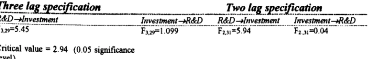
6.3 The Causality Between R&D and Investment:

Traditional Granger Causality Tests

161

6.3.1 Unit Root Tests

162

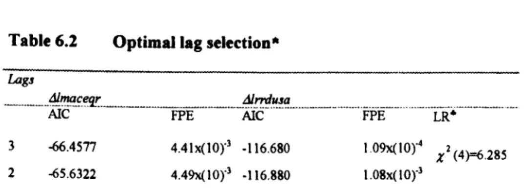
6.3.2 Choosing the Appropriate Lag Length

165

6.3.3 Cointegration and Granger Causality

170

6.4 Causality Between R&D and Investment in an Intersectoral

Framework

176

6.4.1 Time Series Properties of the Variables

182

6.4.2 Long-Run Relationship

188

6.5 Conclusions

191 Appendix 1-

Data Description

193 Appendix II - Data Sources and Summary Statistics

202 Appendix III - Investment and R&D Growth Rate

205

7. The Interaction Between Investment and Output Growth

208

7.1 Introduction

208

7.2 Traditional Granger Causality Tests

210

7.3 Long-Run Relationship

213

7.4 The Dynamic Response of Output Growth

216

7.5 Conditional Granger Causality

(R&D, Investment, Output Growth)

219

7.6 Conclusions

224 Appendix -

Data Sources and Summary Statistics

226

8. R&D, Investment and Growth: the UK Evidence

227

8.1 Introduction

227

8.2 Causality Between R&D and Investment

228

8.2.1 Unit Root Tests and Traditional Granger Causality Tests

228

8.3 Long-Run Relationship

231

8.4 The Interaction Between Output and Investment

233

8.5 Long-Run Relationship

236

8.6 Conditional Granger Causality

(R&D, Investment, Output Growth)

238

8.7 Conclusions

240 Appendix -

Data Sources and Summary Statistics

242

9. Conclusions

243

(6)

Summary

The thesis presents a critical review of both traditional and new growth models

emphasising their main implications and

points of controversy. Three main research

directions have been followed, refining hypothesis advanced in the sixties. We first find

models which follow the learning by doing hypothesis and therefore consider knowledge

embodied in physical capital. The second class of models incorporate knowledge within

human capital while the third approach considers knowledge as generated by the research

sector which sells designs to the manufacturing sector producing capital goods. A typical

outcome of such models

is the existence of externalities which causes divergence

between market and socially optimal equilibria. Policy intervention aimed at subsidising

either human capital or physical capital is thus justified.

Empirical analysis has received new impetus from the theoretical

debate.

However, past empirical tests

are mainly based on heterogeneous

cross section data

which take into account mean growth rates over given periods of time, and ignore pure

time series analysis. On empirical grounds, the role of investment in the growth process

has been emphasised. This variable has also been decomposed to consider the impact of

machinery and equipment investment alone.

In this thesis we have underlined six

aspects of endogenous growth models,

which in our opinion reflect the main points of controversy:

i) scale effects;

ii) the treatment of knowledge as a production input;

iii) the role of institutions;

iv) the empirical controversy dealing with the robustness of growth regression

estimates and the measurement of the impact of some crucial variables (e. g.,

investment) on growth;

v) the simplified representation of R&D;

vi)

the absence of any discussion of diffusion phenomena.

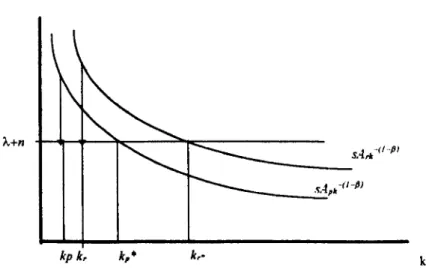
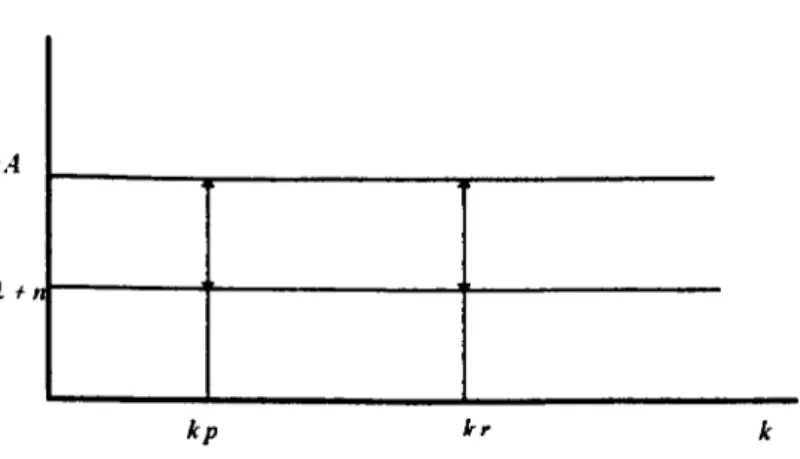
We then propose a new version of an R&D endogenous growth model, which

explicitly incorporates the diffusion of innovations and permits comparison with results

derived from other models which do not consider the diffusion process. In this new

model the interaction between the sector producing final output and the sector producing

capital goods generates the time path of diffusion and hence the growth rate of the

economy.

(7)

In addition, there is another clear growth effect which derives from changes in the parameter which defines the diffusion path of new capital goods.

An

increase in the value of this parameter again causes an increase in human capital devoted to research and an upward shift of the diffusion path, thus increasing the long-run growth rate. This result underlines the difference with previous R&D endogenous growth models in that we now have a clear distinction between the sectors producing and using new capital goods.

The empirical implications of the theoretical models are then investigated by testing the causal link between R&D and investment, on the one hand, and output growth and investment on the other hand. Indeed, a crucial task of any empirical investigation dealing with endogenous growth theories is to explain the nature of the links between industrial research, investment and economic growth. There is much room for study in this framework, as there are still only a few studies analysing these relationships. Our analysis deals with both aggregate data for the US and UK economies and an intersectoral analysis for the US manufacturing sector. We have used a test procedure which allows us to analyse both the short-run and the long-run properties of the variables using cointegration techniques. We are able to test for any feedback between these variables, thus giving more detailed and robust evidence on the forces underlying the growth process.

The results suggests that R&D Granger causes investment in machinery and equipment only in the US economy. However, there is evidence of long-run feed-back implying that investment may also affect R&D. In the UK economy there is no evidence for R&D causing investment nor is there strong evidence of long-run feed-back between the two variables. This suggests that the causal link between R&D and investment may not be thought of as a stylised fact in industrialised economies.

(8)

CHAPTER

I

1. Introduction

Growth theory has been a central issue in Economics since classical economists.

In the 1950s and 1960s it became the most important issue in economics following seminal studies by Schumpeter (1934) and Solow (1956). Solow's neo-classical

approach contributed to resolving controversial results from previous models (Harrod, (1939, 1949) and Domar (1946». Studies by Koopmans (1968) and Cass (1965) refined the standard neo-classical approach with a more detailed theoretical framework, while

the studies by Kuznets (1955) contributed to the empirical debate on economic growth. After this period of controversial debate, interest in growth related issues

decreased, due to both theoretical and empirical problems. The main drawback of the neo-classical model lies in the assumption that technological change is exogenous and as a result the model cannot discriminate between the different variables which cause long-run growth. This analytical drawback contributed to a decrease in interest, both

theoretical and empirical, in economic growth until the first half of the 1980s, when new

models were proposed building on the seminal work by Arrow (1962), which endogenised technical progress through a learning-by-doing approach.

(9)

2

Knowledge becomes the crucial element in the innovative process with the new growth theory considering its role incorporated in either physical or human capital. This new analytical approach refines the neo-classical model and the studies by Arrow (1962) and Uzawa (1965). Some of the new models also consider knowledge as the result of the specific activity of an R&D sector in the economy. In such models technological

progress is endogenised through the production function of the R&D sector., the parameters of which determine, therefore, the long-run growth rate of the economy. A

typical outcome of such models is an externality associated with knowledge, as it is not a

fully excludable good. Thus, the market equilibrium may diverge from the welfare optimum, depending on the nature of the knowledge generating process. Such

externalities may affect either human or physical capital but in all cases the outcome is a

remuneration of human capital or physical capital which is less than is socially optimal. Despite recent analytical improvements there is still a gap between theoretical predictions and empirical findings. The empirical results (which are typically based on new data sets for the world economies (Penn World Table» often contrast with the conclusions of the theoretical models and, in general, there has been no improvement in the explanatory capacity of these models compared with the traditional neo-classical model. This fact is crucial, as it may reduce future interest in growth theory and hence in

the explanation of the determinants of long-run growth.

Together with the new interest in growth issues, there has also been a growing

interest in the economics of innovation. Building upon the work by Schumpeter (1939),

(10)

3

However, there is still a wide gap between the analysis of new growth theory, which endogenises the innovation process, and the economics of technological change. In particular we think that the analysis of the diffusion process in the innovation field may be used to help understand the possible impact of innovation on output fluctuations within the analytical structure of endogenous growth models. Hence, in this thesis, we

have incorporated an explicit treatment of the diffusion of innovation into an aggregate

endogenous growth model. Both theoretically and empirically, we have then analysed in depth the implications for the aggregate model, focusing on the causal links between the

key variables within the model, i.e., R&D, investment and output growth.

The thesis is organised as follows. In the second chapter we critically review both

traditional and new growth models. We focus particularly on the R&D endogenous growth models (Romer 1990a, I990b, Grossman and Helpman 1991a, 1991b) which represent the theoretical framework used later to incorporate the diffusion process into an aggregate growth model. We also analyse the empirical evidence relating to such models.

The third chapter analyses the theory of technological diffusion, focusing on both

(11)

4

In the fourth chapter, we present a new version of an R&D endogenous growth model, which explicitly incorporates the diffusion of innovations and permits comparison with results derived from original models which do not consider the diffusion process.

The last three chapters present empirical results. This are mainly concerned with tests of the main predictions of endogenous growth models, i.e., the causal link between

R&D and investment, on the one hand, and output growth and investment on the other hand.

This analysis sheds light on relationships which are still controversial within the

empirical debate and may help in our understanding of the empirical implications of the growth models analysed in the previous chapters. The analysis deals with both aggregate

(12)

5

CHAPTER II

2. Technological Change and Endogenous Growth

2.1 Introduction

The determinants of economic growth have always been a point of controversy in

economic debate. In this chapter we shall analyse the main theoretical and empirical studies which have significantly contributed to the debate on economic growth and focus on the research lines representing the benchmark for the analyses described in the follow-ing chapters.

In the initial stages the theoretical debate concentrated mainly on the use of an aggregate production function to represent the economy and the growth rate was taken

as exogenous, given an exogenous growth rate of the population and technical progress. Debate on these issues, which ceased for roughly twenty years, received further impetus from a new theoretical perspective which tends to focus on the variables endogenously

determining the growth rate, and may therefore explain the long-run differences between different economies. A starting point for this debate is provided by Romer's analysis

(1986), in which the growth rate is endogenously determined following a learning-by-doing approach (Arrow 1962). Since then new models have been developed,

concen--

.

(13)

6

in the original Arrow model, or in human capital (Uzawa 1965, Lucas 1988). In addition,

technical progress may be endogenised considering a third approach providing a specific sector of the economy (Research and Development) which produces knowledge which may then be used to produce new capital goods.

These new elements of the debate will be analysed, with particular emphasis on

their implications.

It

will be useful, however, to start this analysis with a brief review of

the traditional models, and then move on to analyse the new approaches in greater detail.

2.2 An Overview of Traditional Growth Models

2.2.1 Harrod-Demar

We shall start the analysis of the traditional approaches with the Harrod-Domar model'. We can summarise the model briefly as follows:

(2.1)

L

J =

Loe

nt (2.2)

I=S

(2.3)

S=sY

(2.4)

_I

₌

V(~)

(14)

7

Equation [2. I] represents the labour supply. It is assumed that the labour force

grows at an exogenous and constant rate equal to

n,

while [2.2] represents the

equilib-rium conditions on the goods market. Savings [2.3] are a constant proportion of the

na-tional income (Y). Equation [2.4] implies that, along a growth path where the goods

market is in equilibrium, expectations are always fulfilled: in other words, at any time

t,

firms will invest as long as the equilibrium between the desired and effective capital stock is reached. Recall that v represents the desired capital/output ratio and dy

at

the

ex-pected change in income. Along a balanced growth path, the expected and effective growth rates coincide.

In this context, without technical progress, the output growth rate coincides with

the growth rate of the labour force (n):

(2.5)

(2.6)

• y

=n

y

where

Y

=

dY

and." is the labour-output ratio. Technical progress may be introduced

dt

assuming that

it

is neutral, labour augmenting and growing at a constant rate 2.

We therefore have

2 Recall that the neutrality of technical progress referes to three different concepts:

(15)

8

where s,is the growth rate of technical progress. Equation [2.7] establishes that the

la-bour-output ratio decreases (due to technical progress) following an exponential path

determined by the parameter

ga'

Output dynamics is therefore determined by the parame-ters 11and

ga:

(2.8)

We therefore have

(2.9)

.

y

- =g +11

Y a

Equation [2.9] shows the natural growth rate when technical progress is included

in the model. From [2.3] and [2.4] we get the definition of the warranted growth rate

which maintains the goods market equilibrium. Thus we have

(2.10)

v-=sY

dY

dt

(16)

9

(2.11) ldy

₌

s

y dt v

Equation [2.11] implies

The warranted growth rate is sv. Therefore, a balanced growth path is only reached when s/v = n -+-

ga ,

i.e., when both per-capita income and per capita-capital

stock grow at the exogenous rate

ga,

which is determined by technical progress, and full employment is guaranteed. However, s and v are not endogenous variables and, there-fore, there is no guarantee that the equality between the natural and warranted growth

rates is reached in the economy.

The solution of this dilemma in the Harrod-Domar model has been twofold. On the one hand, the post-Keynesian school has emphasised the endogenity of the saving propensity considering its diversification among the social classes (Pasinetti 1962, 1974). On the other hand, the neo-classical approach (Solow 1956) has used the definition of aggregate production function to enodogenise the capital-output ratio.

2.2.2 The Neo-Classical Model

(17)

10

therefore, the capital-output ratio may vary as well thus modifying the assumption of the Harrod-Domar model in which the capital-output ratio is fixed.

The economy may be represented by means of an aggregate production function of the type

(2.13) Y

=

f(K(t), A(t)L (t»

where

K

represents the aggregate capital stock,

L

the labour force and

A

a variable which

incorporates the change in labour productivity. It is assumed that

A

is an increasing and

monotonic function of time. Equation [2.13] may be written in terms of output per

effi-cient labour units

(2.14) y

=

f

tk )

==

l(k,l)

f'

(k) >

0;

I"

(k)

s

0

where

It is also assumed that labour productivity grows at a constant rate

go

and the

growth rate of the labour force isn. This means that 1

(2.15) A(t)

=

egG/

(2.15') L(t)=e'"

(18)

11

If the previous hypothesis that each individual saves a constant ratio

s

of hislher income is maintained, aggregate savings are given by

(2.16) S=sY

Savings are used to finance investments, and assuming no capital depreciation,

we get

•

(2.17) K =sALj(k)

Combining [2.15], [2.15'] and [2.17], we may write

•

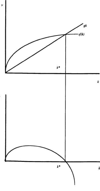
(2.18) k =sj(k)-(g" +ll)k

This equation is a version of the well-known fundamental equation of the Solow model, which determines the evolution of the capital-labour ratio.

When s/(k) is greater than (ga + ll)k, the capital-labour ratio grows, while on the

other hand k decreases when s/(k) < (ga + n)k. Figure 1 shows the equilibrium path of

(19)

12

y

gk

k

•

k

(20)

13

2.2.3 Optimal Growth

The traditional neo-classical model may be modified to endogenise savings and to de-termine the optimal growth rate, which, without external effects and assuming rational

expectations, coincides with the competitive market equilibrium. The theoretical framework is a synthesis of the analysis of Ramsey (1928), Cass (1965) and Koopmans (1965).

The representative individual has a utility function of the type

(2.19)

Cl-Cl -1

U(C)

=

---,-t_

I-a

where

C

is consumption at time

t

and a defines the intertemporal elasticity of

substitu-tion. The representative consumer chooses the consumption path which maximises the

utility function [2.19], under the constraint of the available resources. Itis assumed that

the aggregate production function is of the type Y =/(K(t),A(t)L(t)). This equation may

be written in terms of output per efficient labour unit, as in the case of [2. 14]. The

in-tertemporal maximisation problem may be formulated as follows:

00 ((

=r:

1)

(2.20)

Max

f

«<r:"

ce; _

a -

dt

o

s.t .

•

(21)

14

where c is consumption per efficient labour unit, p is the rate of time preference,

n

the

population growth rate, ga the productivity growth rate and A.the capital depreciation rate 4.

The corresponding Hamilton conditions of this problem are

(( ceg.1

r:

-1)

(2.21)

H=e-(p-n)1 +m(f(k)-c-(ga +n+A)k)

I-a

(2.21')

He

=

0<::> e-(p-n)t

e

gat

(ce

gat

Fa -

m

=

0

•

(2.21" ) H, =+m<::> -m(

f'

(k)-

(s,

+n+ A)) (2.21"') lim m(t) =Ojlim H

=

0

t~1X') t--+(1)

where m is the co-state variable. Taking logarithms of [2.21 '], differentiating with

re-spect to time tand combining with [2.21 '], we get the growth rate of

c:

• c

(2.22)

-=a-1(f'(k)-(ag +A+p))

c a

The inclusion of exogenous labour productivity growth enables us to solve the problem of the constancy of per-capita income and consumption in the original neo-classical model.

(22)

15

In this case, in steady state, the ratio ~

=

C , i.e., per capita consumption in efficient

AL

labour units, is constant. However, per capita consumption in physical units grows at

the rate

ga

since [2.23] holds:

c

-(2.23)

-=cA

L

If this result solves the problem of the cap on per capita income and consumption

typical of the neo-classical model without technological change, it does not, however, explain the source of technical progress and therefore the source of economic growth. This contradiction in the original neo-classical model, which, in fact, represents the real objective of a theoretical investigation on growth, has been faced by the later endoge-nous growth models. This line of research aims at investigating the source of techno-logical change and its impact on growth and on the ability of the market economy to

reach efficient growth paths.

2.3 Endogenous Growth Models: the role of knowledge

2.3.1 Learning by Doing

(23)

16

Endogenous growth models have tried to fill this gap by defining the variables which may affect technical change. However, the theoretical framework of this line of research lies in models refined in the 60s (Arrow 1962, Uzawa 1965, Shell 1966), in

which the role of knowledge as production input is considered. There has been three main lines of research which have tried to identify the mechanisms of knowledge

accu-mulation.

Firstly, knowledge has been incorporated in physical capital (Arrow 1962),

de-pending on its accumulated stock. The rationale of this analytical tool is that firms im-prove and add knowledge (learning-by-doing) to the capital goods they produce. This knowledge incorporated in capital goods may be freely used by other firms, thus

con-tributing to the productivity of production inputs in the whole economy.

Secondly, knowledge has been incorporated in human capital (Uzawa 1965, Lu-cas 1988). Again there may be an external effect (however, not essential to determine an endogenous growth rate of the economy), deriving from the use of human capital in the production process, which, as in the case of learning-by-doing, creates the typical

prob-lem of market equilibrium with externalities.

Finally, there are models (R&D models) which consider knowledge accumulation

as the result of an activity specifically dedicated to this purpose (Shell 1966, Romer 1990a, 1990b, Grossman and Helpman 1991). We initially consider the first type of model then discuss the other theoretical approaches.

We shall start by analysing the non-vintage version of the Arrow model, which simplifies the exposition while leaving unchanged the conclusions (Sheshinski 1967). Consider a

(24)

17

(2.24) Y

=

Kb

A(t)LI-b

where A(t) represents the state of knowledge at time t. Following the learning by doing

hypothesis, we may write

where I( represents the state of knowledge, which is a function of accumulated

invest-ment. As in the traditional neo-classic model, it is assumed that consumers intertempo-raly maximise their utility function. Thus we have

(2.26)

MaxI'"

e-

P1

(c

t•a -I

)dt

1-0 o

s. v.

From the Hamilton conditions we get

t-a

(2.27) H =e-P1(_c-)+m(kfiKI:J. -c)

1-0

(2.28') He

=

0

<=>

e-

P1

c-

a

=

m

• •

(2.28") Hi; = - m

<=>

m=-m(f3k -(1- filKI:J. )

(25)

18

where leis the aggregate measure of capital stock,

k

is per capita-capital stock and

L

is

the labour force.

The equilibrium condition in the capital market requires that

K=Lk.

Taking logarithms of

[2.28'], differentiating with respect to time

t

and finally substituting [2.28"], we get

•

(2.29) ~

=

Y

=

(J -I

(J3k

-(I-I1-~)

La -

p)

C

This condition states that the consumption growth rate is proportional to the dif-ference between the marginal product of capital and the rate of time predif-ference. In this

version of the model it is assumed that the labour force is constant.

Itis worth noting that this model shows an endogenous growth rate

r

> 0

pro-vided that

f3

+ a

=

1. If we consider a logarithmic transformation of [2.29] and

differen-tiate with respect to time

t,

we get

(2.30) 0

= f3(a

+

f3

-l)y

If a+

f3

< 1, the only steady state growth rate is

r

=

0, as in the traditional

neo-classic model without technical progress.

This result suggests that even with increasing returns to scale a positive steady

state growth rate is not always attainable. In fact, the value of

a

must be sufficiently

(26)

19

In this case the growth rate would be'

This growth rate implies a scale effect which derives from the size of the labour

force. This effect depends on the assumption that knowledge is incorporated in the

ag-gregate stock of capital. On the other hand, if one assumes that knowledge is proxied by the average capital stock, a growth rate independent from the size of the labour force

may be derived'

The market and optimal equilibria differ since the social planner would maximise

the utility function [2.27], no longer assuming the stock of knowledge (incorporated in

the capital stock) as given. The first order conditions are therefore obtained including all

capital stock, even that part which is external to the individual firm. The Hamilton

conditions become

1-0

(2.32)

H =e-P'(_c_)

+

m(ka+~La - c)

1-(J

.

(2.32")

n,

=-m<;:::>m=-m((a+~)k-(1-a-~)c')

(2.32"')

limmit )

=

0;

limH

=

0

I~OO 1400

This implies the following growth rate

5Romer (1986) has shown that a technology with increasing return to scale such that ~+<x>l may cause

a positive and growing growth rate.

(27)

20

This growth rate is higher than the market equilibrium growth rate. In other

words, the competitive equilibrium implies an underinvestment by the single firm, since it

does not internalise the externality represented by the stock of knowledge incorporated in physical capital. This underinvestment therefore causes lower production.

We may link this analytical approach, which incorporates the stock of knowledge

m physical capital, to a wider field of investigation, where the so-called learning by watching is taken into account (King and Robson 1989, 1992).

The basic idea in this framework is that there is a demonstration or contagion

ef-fect which comes from observations of new ideas embodied in new investment The em-pirical evidence discussed in Cohen and Levinthal (1989) shows that many innovations in one firm or industry determine development and innovations in other firms and

indus-tries. Scott (1989) views investment as the engine of growth, because it brings about new investment opportunities, which may be called learning externalities. In the model proposed in King and Robson, the level of technological knowledge evolves over time

(28)

21

Denote

G;

as the natural growth rate given by the technical progress function, which is a

function of the investment rate (i):

(2.34) G,

=

f(i)

From the intertemporal maximisation problem one can derive the growth rate of

consumption'

c (r -p)

(2. 3 5)

= ;_______::_:_

C 0'

where

p

is the rate of time preference, r is the interest rate and adefines the

intertempo-ral elasticity of substitution.

The investment criterion adopted by firms requires that the marginal product of

capital be equal to its user cost. Assuming a Cobb Douglas technology, the production function in per capita terms is:y=Al-ak, where A represents the stock of knowledge and k

per capita capital. It is assumed that the labour force is constant and this allows the normalisation

L

=

1. Knowledge is a function of investment and evolves according to

The investment criterion condition implies

'Given a utility function of the type

.

U(c)=C1-erlI-o .from the intertemporal maximisation of this

.

c

(r-p)

function one gets: -

= --_

...

(29)

22

a

r

(2.37) -= -+A

v

1-1

where

v

is the capital-output ratio,

r

is the interest rate,

A.

is capital depreciation and Iis

the tax rate'.

Equilibrium requires that [2.34] and [2.35] be equal, i.e., the natural growth rate

and the warranted (rational expectation) growth rate must be equal. Furthermore, in equilibrium the investment rate is given by

(2.38) I.=-vC

c

Solving the system represented by equations [2.35], [2.37] and [2.38], gives the equilibrium growth rate

•

c

i(p+'A(I-I))

(2.39)

-=y=----c a(l-I)-oi

Itis worth noting that this solution is not unique given the non-linearity of the

technical progress function. Equation [2.39] states that the growth rate compatible with

(30)

23

capital market equilibrium is an increasing and convex function of i. The equilibrium solutions are given by the intersections with the technical change function (Figure 2.2).

r

CJlE

TPF

Figure 2.2

CME=Capital market equilibrium

TPF=Technical progress function

2.3.2 Knowledge and Human Capital

(31)

24

scale. The labour input is allocated between the education and production sectors. The

aggregate production function is of the type: Y =I{K.AL). The model may be

summa-rised as follows:

00

(2.40) Max

J

e( t )e -pidt

o

•

(2.40' ) k

=

.ry - Ale

(240")

A

=

A'It:J

where e is per capita consumption. A the state of technological knowledge. A.the capital

depreciation rate,

s

the proportion of savings to national income and

y

per capita income. In other words, the problem is the usual intertemporal maximisation of con-sumption subject to the constraint determined by the accumulation of physical capital

and technology. The latter is a function of the ratio between the labour force employed in the education sector (LE) and in production (Lp). Itis worth stressing that the division of the labour force into two components has been widely considered in many later en-dogenous growth. models.

It

is possible to derive the optimal allocation of the labour

force between the production and education sectors and the optimal capital-labour and capital-output ratios from the conditions for intertemporal maximisation. In the model it is shown that the optimal growth rate is reached when the growth rate of labour

pro-•

(32)

25

Following the line of research outlined by Uzawa is the Lucas model (1988), which represents a generalisation of the previous models of human capital accumulation. Consider again a closed economy with competitive markets, identical individuals and a technology with constant returns to scale in absence of externalities. We also define

h

as

a measure of the qualification of each worker. It is assumed that a worker with this qualification level assigns a fraction q(h) of his/her time to productive activity and a

frac-tion 1 -q(h) to hislher qualification.

In addition to this direct effect of human capital on productivity, an external ef-feet is considered. This latter refers to the mean level of qualification of human capital, which may also influence the productivity of other inputs and therefore may affect the growth rate of the economy. As in the previous model it is assumed that consumers

maximise their utility

in

an infinite time horizon. We then have

(1) I-a

(2.41) Max

f

~pI L(t)dt

o I-a

• f\S

(2.411) K =AKf3[qhLtf3 h - Le

•

(2.41") h

=

Eh(l-q)

It is also assumed that the labour force grows at an exogenous rate n.

(33)

as-26

s

sumed that the technological level is constant and equal to

A.

The term h captures the external effect of human capital and is proxied by the mean qualification level of the la-bour force. The second constraint concerns the accumulation of human capital. This

equation implies that the accumulation of human capital is a linear function of the effort

dedicated to this accumulation process (1 -q).

If there is no effort in the accumulation of human capital (q

=

1), the economy does not accumulate human capital. On the other hand, if

q

=

0, i.e. the entire effort is

dedicated to the accumulation of human capital, the economy grows at the rate E. The

~ iJ

equilibrium condition in the labour market means that h =h.

The conditions which show the growth rate of per capita consumption and human capital can be derived from the Hamilton conditions.

(2.42) H

=

e-

p,(

cl-a)

L(t)+m(AKP

(qL)H

hl-P,S -

Le)

+

l(hE(1- q))

1-0

(2.42') He =0

<=>

e-p'c-

a =

m

(2.42" )H

q

=

0

<=>

m(

AKP

(1-

f3)(

qLhr

P

LhI+

S)

=

lthe )

(2.42'" )H

le = -;"

<=>;"

=

-m(f3AKP-1

(qL/-

P

h

l-

P

+[})

(2.42'" )H

h

=

-i

<=>

i

=

-m((1-f3)AKP

(qLY-

P hH+S )-1£(1-

q)

From conditions [2.42'] and [2.42"] it is possible to derive the equation which

(34)

27

(2.43) ~

=y =0'-I(I3AK[3-1 (ql.)I-Ph1-[3+3- p)

e

The accumulation rate of physical capital may be obtained from the constraint

[2.41]

and from

[2.43r

•

K

(2.44)

-

=

y

+n

K

One should consider now the accumulation of human capital From

[2.43]

we get

(2.45)

(y~:

p)

=

KP-1(qL/-P

hl-P~3

Taking logarithms of

(2.45)

and then differentiating with respect to time yields:

.

h

y(l-I3)

(2.46) h =

(1-13+3)

.

9 . K AK-(1-P)( L 1-Ph1-P.3 Le

Equation (2.44) is derived considering that: - = q )

-K

K

e

The first term on the RHS may be substituted considering the expression for - Therefore we have:

e

.

K

ay

+p

= ----'-____:~

K

13 Le

K

.

K

Taking logarithms and differentiating with respect to time we get: - =

r

+

n

(35)

28

ters which determine the growth rate in [2.46] may be obtained from the Hamilton

con-ditions. In fact, from [2.42"] we have

(2.47)

m

=

E

/

AK[3(qLr

P

Lh

9-P

Again using logarithms and differentiating with respect to time we get

.

. .

m

h /

(2.48) -

+J3y

+Il

+(3 - J3) -

=

-m

h

I

From equation [2.42'''] we note that

m

=

-(p + YeT), while from [2.42"] and

m

.

[2.42""] we may obtain!

= -

6 .Therefore we can substitute these values in [2.48] to

de-I

scribe the parameters which define the growth rate of human capital

h _

_

(1-J3)(t-(p-n))

(2.49) - - Yh -

.-h 0(1-

J3

+

3) - 3

(36)

29

(2.50) e-(p-n)

Y

=

Y

h

= _

__;_--(J

This growth rate coincides with the optimal growth rate. If

s

>0,equation [2.49]

holds and hence we have

r

>

rh.

This will induce higher growth of physical capital

compared with human capital. In a market economy, therefore, with a positive external effect individuals will invest in human capital at a lower rate than would be socially

op-timal. Itis however worth noting that the external effect on human capital is not neces-sary to determine the endogenous growth rate of the economy. This latter is positively influenced by the parameter which defines the productivity of human capital, the growth

rate of the labour force and the intertemporal elasticity of substitution. The growth rate is negatively influenced by the discount rate.

2.3.3 Endogenous Growth and Research and Development

In this type of models knowledge accumulation explicitly depends on the amount of resources allocated to inventive activity. A common framework for the recent models described by Romer (1990a, 1990b, 1991) and Grossman-Helpman (1991, 1992) is the

original work by Shell (1967). The economy is again represented through the aggregate production function

(37)

30

where

K

and

L

are respectively the capital stock and the labour input.

A

is the aggregate stock of knowledge. The evolution ofA is given by the following equation

.

(2.52)

A

=oy,(t)Y -

AeA

O<o~l

O~yr ~

1 x,

~O

where 8is a coefficient which reflects the success of the research activity,

v.

indicates the

proportion of output allocated to inventive activity and A..: is the rate at which techno-logical knowledge is depreciated.

The aggregate stock of capital evolves according to

(2.53)

K

=s(tJ[l- y,(t)]Y-')J(

where srepresents the propensity to save and A is the capital depreciation rate. We focus

on the accumulation of

K

and

A ~

it is therefore assumed that the labour force is constant and normalised to one. In a decentralised economy the accumulation process may be

obtained from the system [2.52] [2.53].

(38)

31

00

(2.54) Max

j

U[(l- s)(l-

Yr

)Y, -pidt

o

(2.54' ) (2.54")

•

A

=

0YrY -AeA

.

K

= s(l-

Y

r )

Y -

').J(

The usual Hamilton conditions may be derived. However, it must be stressed

that when there are two state variables (A and K), the solution of the problem is not simple. Shell does not give an explicit solution; however, he shows how

A

and

K

tend to

-

-a specific const-ant, respectively A and K .

This result is not consistent, since bounded technological progress can only guarantee a constant income level which therefore remains steady. This criticism, dis-cussed in Kzuo Sato (1965), is based, in particular, on the specification of

A.

In fact, if

[2.52] is rewritten as

.

(2.55)

A

=

0YrA - ArA

or

•

(2.56) A

=

OV -

A

A :.Tr r

then there is no longer an upper bound to knowledge as long as oYrAr> O.

(39)

32

In the Romer model, the output of the sector which produces knowledge is a partially excludable good. It should be borne in mind that a good is rival if its use by an individual or firm precludes its use by another. The opposite definition applies for non-rivalry. A good is excludable if the owner can prevent others from using it. Public

goods are, by definition, both non-rival and non-excludable. The Romer model separates

the rival and non rival component of knowledge. The former is proxied by human capital used in the production of consumer goods, while the latter is proxied by the stock of

knowledge incorporated in the designs of the existing capital goods.

The economy is represented by three sectors:

a) the final goods sector;

b) the research sector;

c) the sector which produces capital goods.

In the first sector the production function considers a multiplicity of capital goods

using a representation taken from Dixit and Stiglitz (1977):

~

(2.57) Y= g(L.

HyJL

x(il

1=1

(40)

33

X

==

{X

I }: l' The production function is homogeneous of degree one. The function

g(Hy.L ) is therefore homogeneous of degree I - f/J.

The production function describes the technology of a representative firm, within a competitive market.

The research sector produces knowledge, which is incorporated in designs then sold to the sector which produces intermediate goods. The production function in this sector considers the production of designs at time t as a linear function of human capital

(Ha) and the existing stock of knowledge (A)

•

(2.58)

A=oHuA

where 8 (8 > 0) is a parameter reflecting the productivity of human capital in the

re-search activity. The sector which produces intermediate goods cannot be described in terms of a representative

firm.

For each capital good (t) there is a distinct firm which therefore acts as a monopolist.

A firm in the manufacturing sector may convert J.Junits of final output into a unit

of intermediate good . The aggregate measure of capital (K)may be defined as follows:

A

(2.59) K

=

I!

LX,

(41)

34

where p represents the cost (in terms of final output) of producing one unit of capital

good (i). The total amount of human capital H is the sum of human capital in manufac-turing (Hy) and human capital employed in the research sector (Ha.). Itis also assumed that the labour force is constant, implying that H and its components are constant as well.

It is then assumed that the different types of capital goods are all used at the same level

x·

and that the index i may be represented through a continuous variable. Equations

[2.57] and [2.59] may be rewritten as follows:

where

x·=-

K

/J

A

and

(2.61)

K=/J Ax·

(42)

35

O.

Due to the stationarity of the model the values of

Ha

and

H,

are constant; however,

the value of

Ha

is endogenously determined, thus also determining the growth rate of the economy.

The labour market must clear for

Ha

and

H,

to remain constant. and, therefore,

returns on human capital employed in the manufacturing sector and in the research sec-tor must be equal. In the manufacturing sector returns on human capital are given by

the marginal productivity rule. We therefore have

(2.62) W.fly

=

gflyA( x*l

where Whyis the remuneration of human capital and ghyA(x*)¢Jis its marginal

pro-ductivity. In the research sector, returns to human capital depend on the rent which can be extracted from a patent on an invented capital good. Thus we have

(2.63) Wfl

=

P»A

•

where P; is the present value of the monopoly rent which can be extracted by researchers

and

oA

is the number of designs produced per unit time per unit human capital. The

(43)

36

A

(2.64) Max

J

(g( Hy,

usar :

p(x(i))x(i))di

o

and therefore

(2.65) p(x(i)) = q,g(Hy, L)x(i)CP-1

On the supply side, given the demand function, the problem for the single monopolist

which produces capital good (i)is

r

A

f

rt sIds

(2.66) Maxf[p(x(t))X(t}-r(I)J.IX(I/r 0 dt

o

where rp.(t) is the rental cost of capital used for the production ofx(i). This problem is,

however, easily solved due to the stationarity of the model. Indeed, r, x(i) and pare

constant in equilibrium. The cost of a patent Pa will be defined in equilibrium by

(2.67) P,

=

X

*

rm

1

~f

(44)

37

1

(g( H .

L)cp2J

1-<1>

(2.68)

x·

=

y

rJ..l

The conditions for the equilibrium in the labour market are

If for the sake of simplicity and without loss of generality we explicit the function

the value of

Ha

may be endogenously determined.. If we take preferences as being

ex-ogenous, this value will be given by

H =H-

ra

(2.71) a df

If we endogenise preferences, the value of

Ha

is determined

by"

10Preferences are easily endogenised through the usual intertemporal maximisation: Max (Cl-U/l-a)e-rt

.

C

(45)

38

(2.71' )

In both cases the result is crucial for it shows that the balanced growth rate depends on

the allocation of

Ha.

which is in turn obtained from the equilibrium conditions in the

la-bour market and from the parameter 8, which represents the productivity of the human

capital employed in the research sector. Equation [2.71] suggests that a decrease in the

interest rate causes an increase in

Ha

and therefore has a positive effect on the long-run

growth rate. From equation [2.72] the impact of the interest rate is obtained through

the parameters p and

a.

It is worth noting that the parameter p" which defines the

pro-duction cost of capital goods, does not affect the equilibrium value of

Ha

and therefore the growth rate. This means that any investment subsidies, which bring about a reduc-tion of the producreduc-tion cost of capital goods, have no effect on economic growth. This is due to the equilibrium conditions in the labour market. Human capital in the research sector must compete with human capital in manufacturing and returns on both inputs

must, therefore, be equal in equilibrium. A subsidy which reduces the value of p,

deter-mines a higher value of x* (from equation 2.67).

An

increase inx* has a positive effect on the marginal productivity of

H,

and therefore on its remuneration. On the other hand, the demand for capital goods increases and returns to human capital in research increases

(46)

39

The growth rate determined through this mechanism is lower than the socially optimal growth rate, as returns on human capital in the research sector do not corre-spond to their optimal level, causing, therefore, an underallocation of resources in this sector. This depends, on the one hand, on externality in the research sector, as the

ag-gregate stock of knowledge grows as new inventions are discovered without any remu-neration (due to the non-excludability hypothesis). On the other hand, the purchase of

designs is made by a single monopolist producing intermediate goods. This causes a difference between the remuneration of the input used (the price of the patent) and the marginal productivity of human capital in the research sector.

A socially optimal solution may be achieved through a subsidy to the research sector to balance the difference between the marginal productivity of human capital and the corresponding remuneration.

2.3.4 Product Variety

(47)

differ-40

entiated good. The firm may also invest in Research and Development to produce new differentiated goods.

The model is characterised by an aggregate demand side defined by

I

(272) C

=

[I

x(j)"d;

r

O<a<l

where xU) is the quantity of good x of the variety

j.

On the supply side, each firm holds the technology for the production of a single variety, for which it has a monopolistic

power. Itis assumed for simplicity that each variety needs a labour unit for each unit of

output produced. The demand function [2.72] implies that:

MRO)

=

aptj),

where

MRO)

is the marginal revenue and

pO)

the price of variety

0).

If the marginal cost

MC

is equal to the wage rate

w

for all varieties and if

MRO)

=

MCU)

the price of the single varieties

will be the same

w

(2.73) p

=-a.

Given the price rule, operating profits per variety of good are defined by

(2.74) 1t=(l-a)pX

(48)

41

where X represents aggregate output and n the number of varieties. In a dynamic framework, monopolistic competition implies an entry condition determined by a

no-arbitrage rule

(2.75)

.

1t S

-+-=r

S

a

represents the value of a firm, which is equivalent to the present value of the profits

gained at

any

time t. In other words,

a

is given by

, 00 -

J

r( sids

(2.76) S

=

Jet

1t(t)dt

where nrepresents the profits flow and r the discount rate. The no-arbitrage condition

establishes that the rate of profit and the rate of capital gain are equal to the nominal

in-terest rate.

A

potential entrepreneur who wants to invest in

R&D

to develop a new

(49)

42

(2.77) 3

=

wb

An

where

b

is a parameter which reflects labour productivity,

w

is the wage rate and

An

is

the stock of knowledge.

Assuming that

An

is proxied by the cumulated experience

in

R&D measured by the number of varieties which have been invented

(n),

we may write

II

(2.78)

S

=

wb

n

The equilibrium condition in the labour market requires that employment in R&D

and in the manufacturing sector be equal to the aggregate supply of labour

(2.79)

!!_~+

X

=

L

n

where

bill

represents the amount of work needed for an innovation; ~ is the number of

innovations at time

t

and

X

the amount of labour allocated to the manufacturing sector.

If it is assumed that consumer preferences are described by the usual utility

func-tion

U = --,

c" "

the growth rate of C may be derived from

1 - o

(50)

43

(2.80)

C

=

_![r -

p-

Pc

1 e

a

r.

where

pc

is the price of final output (in equilibrium the price is identical for all varieties).

Given the equilibrium condition in the labour market and the non-arbitrage condition, it

is possible to show that the economy is characterised by the following growth rate"

[ (1- a) ~ - up]

(2.81) Yn

=~--~---u+(1-u)a

where

p

is the rate of time preference,

b

is the parameter which reflects labour

produc-tivity and

a

is the inverse of the elasticity of intertemporal substitution.

It

is worth

not-ing that

rn

increases if

12Consider the following equations: aYn+X=L; -

"

+ -

a

= r .The first equation represents the

re-a

a

wb

source constarint in the labour market, while the second describes the no-arbitrage. Since

a

=

-n

w

1 b

and

Pc

= -.

and taking the wage rate as the numeraire, we have:

Pc

= -

and therefore:

a

= -.

a a

n

a

"X

This implies that: - = -

r

n .In addition we have: - = (1 - a ) - .From the equation which defines

a

ba

e

(I-a) P -(I-a)

the demand for goods we get: -

=

r

n and _c

=

r

n' The interest rate is

the-e

a

Pc

a

1 - a

refore defined by:

r

= P +

r

n -- (er - 1). Substituting into the equation which defines the no-a

(51)

a) the size of the labour force (L) is greater (scale effect);

b)the rate of time preference is lower;

c)the degree of monopolistic power (11a)is greater;

d) the elasticity of intertemporal substitution (1/0-) is greater .

. These results are clearly shown in Figure 2.3., where the steady state conditions are represented. The RR curve represents the resource constraint, while the AA curve represents the no-arbitrage condition. The RR curve has a negative slope as an increase

in the innovation rate (Yn) implies greater employment in the R&D sector and therefore a

decrease in employment in manufacturing. The AA curve has a positive slope as an in-crease in the innovation rate brings about an inin-crease in the effective capital cost,

deter-mined by a higher interest rate and a faster depreciation of the value of the firm. A higher profit rate is therefore needed to undertake the R&D activity. The intersection between the two curves represents the steady state equilibrium.

Figure 2.3 a. shows how growth is constrained, on the one hand, by the availability of re-sources and, on the other, by market incentives. An expansion of the available resources moves the RR curve upwards; a lower rate of time preference moves the AA curve

(52)

x

A

r

Figure 2.38

It is worth noting that the model defines a positive rate of innovation if

Lrb

>

apl(J - a) (from equation [2.81

D.

If this condition does not hold, there is no

endoge-nous growth (Yn)

=

O. The cost of innovation is so high that it discourages any

innova-tion. The solution implies that all the resources are allocated to the production of the existing varieties of goods, without further innovation (new varieties). Figure 2.3a must

(53)

46

x

A

L

r

Figure 2.3b

This analysis, which deals with the production of differentiated final goods, may

be extended to the case of differentiated productions of intermediate goods. The model may also be extended to the case where the increase in quality of new products is taken into account. In this case, the high quality products substitute for the low quality ones. This means that the producers of the low quality goods will not gain any more positive profits and that therefore monopolistic power is not maintained for an infinite time, as

in the case of horizontally differentiated products.

The arbitrage condition is modified to take into account the risk of the investment

(54)

47

As in the Romer model the difference between the balanced and optimal growth rate lies inthe external effect produced in the R&D sector. Indeed, the stock of knowl-edge grows as new varieties of products are created by single researchers without any corresponding remuneration. A Pareto efficient solution may be attained by introducing a

subsidy to the R&D sector to take into account this spill-over effect and to restore equi-librium between the private and social remuneration of labour in the research sector.

A further development of these R&D models is given in the analysis by Aghion and Howitt (1992), of which we mention the main hypotheses and conclusions.

The output of research activity is made stochastic through inventions which

ar-rive following a Poisson stochastic process. In addition, a sort of Shumpeterian hypothe-sis (creative destruction) is introduced, in that the successful R&D activity makes the previous inventions unprofitable. This innovative mechanism finally determines endoge-nous economic cycles. The model, while improving on previous R&D models, does not

consider capital accumulation, as physical capital is not considered in the production functions of the three sectors which define the economy.

2.3.5 Empirical Evidence

(55)

48

Despite this theoretical improvement, empirical tests in this line of research are still controversial. However, there have been some recent improvements in techniques and in the quality of the data sets. Nevertheless, general dissatisfaction persists, particu-larly regarding the robustness of the results and the explanatory capacity of the adopted

empirical models.

Two different approaches have been used for the empirical tests. The first makes use of a historic approach, identifying all those cases where external economies deriving

from the use of certain capital goods have involved significant increases in productivity growth (Rosenberg 1986, Caballero-Lyons 1991).

The second approach uses econometric analysis based on cross-country data,

which aims to establish the significance of appropriate explanatory variables as determi-nants of the growth rate.

We will focus on this second approach, which is the empirical counterpart of the theoretical models analysed in the previous sections. The core empirical literature in-cludes the studies by Romer (1990b), De Long-Summers (1991, 1992), Barro and Sala-i-Martin (1992), Fischer (1992), Mankiw, Romer and Weil (1992), Jones (1995).

In the model proposed by Romer (1990a, 1990b), the crucial variable affecting

(56)

49

This result crucially depends on the assumption that the function g(Hy,L), which

appears in the aggregate production function, is of the type

1-cp (2.83) g(Hy,L)=[aH: +(l-a)LP]p

If the parameter

fJ

tends to zero, we have the usual Cobb-Douglas production

function

(2.84) g( Hy, L) =

n,

o:(1-CPI L(1-O:I(I-CPI

In this case, even assuming some exogenous variations in the labour force (L),

there are no effects on the equilibrium value of

Ha

and, therefore, on the growth rate. In

(57)

off-50

set each other, thus leaving the market equilibrium unchanged.

In this case the increase

in

L

has no effects on the long-run growth rate.

On the other hand, assuming that the value of the parameter

P

is different from

zero, a variation of

L

influences

HQ'

In this case we have

It

may be argued that if

Hand L

are complements

(if

P

is below zero) an increase

of

L

causes a reduction of

Ha

and therefore a reduction in the long-run growth rate.

The empirical model takes into consideration the basic aggregate production

function [2.60], which may be rewritten as a function of

A

and

K

U sing logarithms and differentiating with respect to time gives

y

d

1~

«. )]

L

A

K

(2.87J-=-l

-,1

(58)

51

Denoting the capital depreciation rate as A, the investment-output ratio will be

linked to Kby the relation

(2.88)

~=[(~)(;)]-A

Substituting [2.88] in [2.86] yields:

'\

From the hypotheses of the theoretical model it may be argued that the invest-ment-output ratio does not affect the growth rate of

A;

on the other hand,

L

has a nega-tive effect on this variable.

From equation [2.89] the impact of the investment-output ratio and the size of

the labour force (L) may be derived, However, one needs to assume, on the one hand, that the ratio HyL remains substantially constant over the sample period and, on the

(59)

52

Table 2.1