An empirical study of the efficiency of EA for diffusion simulation

University of Warwick institutional repository: http://go.warwick.ac.uk/wrap

This paper is made available online in accordance with publisher policies. Please scroll down to view the document itself. Please refer to the repository record for this item and our policy information available from the repository home page for further information.

To see the final version of this paper please visit the publisher’s website. Access to the published version may require a subscription.

Author(s): S Peluchetti and GO Roberts

Article Title: An empirical study of the efficiency of EA for diffusion simulation

Year of publication: 2008 Link to published article:

http://www2.warwick.ac.uk/fac/sci/statistics/crism/research/2008/paper 08-14

DIFFUSION SIMULATION

STEFANO PELUCHETTI, GARETH O. ROBERTS

Abstract. In this paper we investigate the eciency of some simulation schemes for the numerical solution of a one dimensional stochastic dierential equation (SDE). The schemes considered are: the Exact Algorithm (EA), the Euler, the Predictor-Corrector and the Ozaki-Shoji schemes. The focus of the work is on EA which samples skeletons of SDEs without any approximation. The analysis is carried out via a simulation study using some test SDEs. We also consider eciency issues arising by the extension of EA to the multi-dimensional setting.

1. Introduction

In this paper we focus on the eciency of the Exact Algorithm (EA), introduced by Beskos and Roberts [2005], Beskos et al. [2006a]. The framework that we consider is that of the simulation of a diusion process, solution of a SDE, whose transition densities are not known. Hence the direct simulation of nite dimensional, or discretised, paths is not feasible. EA is a method that, under suitable conditions, permits the simulation of the discretised diusion process. The novelty of EA is that we are able to simulate from the true law of the diusion process, without resorting to any type of approximation.

Numerical schemes for the simulation of diusion processes have been around for some time, the rst contribution probably being that of Maruyama [1955]. However, before the work of Beskos and Roberts [2005], the exact nature of the simulation was conned to a very small class of diusion processes. The eld of numerical schemes for the simulation of diusion processes is vast and growing rapidly, motivated by the fact that the class of solvable diusions, that is to say diusions for which the transition densities have a known tractable from, is quite small. See however some recent results on the topic by Albanese and Kuznetsov [2005]. Subsequently, the importance of having a method that allows for exact simulation is clear, if not for validating purposes. The cost that we have to pay for this achievement is less obvious. Hence our focus on the eciency of EA.

Some preliminary results on the eciency of EA, in a Monte Carlo scenario, can be found in Casella [2005]. However this paper gives a much more extensive investigation of EA. We initially consider a class of test models that synthesise a range of one-dimensional diusive dynamics that are encountered in real world applications. We thus simulate them using three well known discretisation schemes and EA and we compare the results obtained. The

simulation study is replicated in the multi-dimensional settings where only the eciency of the multi-dimensional EA is examined.

This paper is organised as follows. In Section 2, EA and the three discretisation schemes are briey introduced. Section 3 consists of the simulation study where the eciency of the 4 schemes is studied. The main diculty is comparing a scheme that returns the exact result with schemes that return approximated results. Consequently it is necessary to introduce a comparison criterion that measures a "distance" between the true and the approximated result. We are interested in both the sensitivity of the schemes to the parameters of the test SDEs and the ratio of eciency between EA and the other schemes. In Section 4 the eciency of the multi-dimensional extension of EA is investigated, without any comparison with the other discretisation schemes. Section 5 concludes the paper.

2. The simulation schemes

2.1. The Exact Algorithm. We begin considering a generic one-dimensional and time homogeneous Stochastic Dierential Equation (SDE)

dYt=b(Yt)dt+σ(Yt)dBt 0≤t ≤T

(1)

Y0 =y

where B is the scalar Brownian Motion (BM) and y is the initial condition. The drift

coecient b and the diusion coecient σ are assumed to satisfy the proper conditions for

the existence and uniqueness of a strong solution of (1). LetY be the diusion process strong

solution of (1).

Under the additional requirement thatσ is continuously dierentiable and strictly positive

let

(2) η(u) :=

u

σ−1(z)dz

be the anti-derivative ofσ−1. It follows thatXt:=η(Yt)satises the unit diusion coecient

SDE

dXt=α(Xt)dt+dBt 0≤t≤T

(3)

X0 =x:=η(y) with drift coecient

(4) α(u) := b{η

−1_(u)}

σ{η−1_(u)} −

σ0{η−1_(u)}

2

SDE (3) is assumed to admit a unique strong solution and we denote with Xthe state space of X. The map (2), also known as the Lamperti transform, allows us to consider the simpler

problem of simulating from (3) for a vast class of one-dimensional SDEs.

law of a BM respectively on [0, T] both started atx. From now on the following hypotheses

are assumed to hold

• (C1) ∀x ∈ _{X Q}x

T WxT and the Radon-Nikodym derivative is given by Girsanov's

formula

(5) dQxT

d_Wx T

= exp

T

0

α(ωs)dXs−

1 2

T

0

α2(ωs)ds

where ω∈C([0, T],_X)

• (C2)α∈C1₍

X,R);

• (C3)α2_+α0 _{is bounded below on} X.

An application of Ito's formula to the functionA(u) =_cu_∈

Xα(z)dzresults in a more tractable form of (5)

d_Qx T d_Wx T

= exp{A(ωT)−A(x)}exp

−

T

0

α2_+α0

2 (ωs)ds

(6)

Under the integrability assumption

• (C4)∀x∈_X ηx,T :=EWx

T

eA(ωT) <∞

it is possible to get rid of the (possibly unbounded) term A(ωT) of (6) introducing a new

process Z with law_Zx_T by the Radon-Nikodym derivative

d_Zx T d_Wx

T

=eA(ωT)/ηx,T

(7)

ηx,T =EWx T

eA(ωT)

(8)

We refer to Z as the Biased Brownian Motion (BBM). This process can be alternatively

dened as a BM with initial value x conditioned on having its terminal valueZT distributed

according to the density

(9) hx,T (u) :=ηx,T ×exp (

A(u)− (u−x)

2

2T )

It follows that

d_Qx_T d_Zx T

(ω) = ηx,T exp{−A(x)}exp

−

T

0

α2+α0

2 (ωs)ds

(10)

∝exp

−

T

0

φ(ωs)ds

≤1

(11)

whereφ(u) := (α2(u) +α0(u))/2−l andl := infr∈X(α

2_{(r) +α}0_{(r))/2<∞. Equation (11)}

suggests the use of a rejection sampling algorithm to generate realisations from QxT. However

it is not possible to generate a sample from Z, being Z an innite-dimensional variate, and

Let L denote the law of a unit rate Poisson Point Process (PPP) on [0, T]×[0,∞), and let Φ ={χ, ψ} be distributed according to Φ. We dene the event Γ as

(12) Γ :=\

j≥1

φ Zχj

≤ψj

that is the event that all the Poisson points fall into the epigraph ofs7→φ(Zs). The following

theorem is proven in Beskos et al. [2006b]

Theorem 1. (Wiener-Poisson factorisation) If (Z,Φ)∼_Zx

T ⊗L|Γ then Z ∼QxT

At this stage the result is a purely theoretical, as it is not possible to simulate from the law L. However, in the specic case of φ bounded upon by m < ∞ it is suce to consider

Φ as a PPP on [0, T]×[0, m]. The reason is that for the determination of the event Γ only the points of Φ below m matter. The algorithm resulting from this restrictive boundedness

condition on φ is EA1.

It should be noted that this hypothesis can be weakened or even removed, leading to EA2 (Beskos et al. [2006a]) and to EA3 (Beskos et al. [2006b]) respectively. Both extensions involves the simulation of some functional ofZ or of an event depending onZ which restrict

the range of Z, and by continuity the range of φ(Z).

We briey consider the case of EA3. The probability that the BB Z stays in an arbitrary

interval can be expressed as an innite series only. As a consequence the direct simulation of the minimum and the maximum of Z is not feasible. However, we can rearrange the terms

of this series so that the sequence of the partial sums sn satises the relations:

sn−1 ≤l⇒sn ≥l

(13)

sn−1 ≥l⇒sn ≤l

(14)

where l is the limit value of the serie. As explained in Beskos et al. [2006b] we can consider

an increasing collection of nested intervals {In}_n≥1 which contains the starting and ending values of Z. Due to the behaviour of the partial sumssn we can simulate the value nso that

both the maximum and the minimum of Z are included in a specic In and at least one of

them is included in In∩InC−1. Conditional on this event Rn the range of Z is bounded.

It remains to implement an algorithm to sample from Z |Rn, as we have to compute the

value of this process at the time instances given by the PPP Φ. It is not sensible to use Z

as a trivial RS proposal, the reason being that the number of proposed paths before the rst acceptance has innite expectation. A better RS algorithm proposes from a mixture of two probability measures with equal weight. One of them is the law ofZ conditioned on achieving

its minimum inIn∩InC−1. The other one is the law ofZ conditioned on achieving its maximum in In∩InC−1. Crucially, it is possible to sample the constrained minimum (or maximum) m of Z and the time τ at which Z hits this minimum (or maximum). Moreover Z | m, τ gets

factorised in the product measure of two 3-dimensional Bessel bridges, whose simulation is trivial. As the Radon-Nikodym derivative of this proposal with respect toZ |Rnis available

2.2. Optimisation of EA. From a practical point of view, every version of EA require the simulation from the density (9). This is not a trivial problem as the functional form of (9) depends on the drift coecient α in (3). Moreover, theoretical results (see Beskos et al.

[2006a]) suggest that the acceptance rate of EA typically decreases exponentially with T. It

turns out that it is usually more ecient to partition the time interval [0, T] into smaller sub-intervals of length t and apply EA sequentially. This in turn implies that we have to

sample from a parametric family of densities{hx,t(u)}_x∈_X, as the starting valuexis dierent

on every sub-interval.

Furthermore the time spent in the simulation from {hx,t(u)}_x∈X is not negligible in EA. In the particular case of EA1 roughly half of the time is spent in the simulation from

{hx,t(u)}_x∈X. Thus an ecient sampler results in a signicantly lower computational cost for the EA. We briey introduce two adaptive accept-reject samplers that we have developed to sample eciently from {hx,t(u)}_x∈X and we refer to Peluchetti [2007] for a more detailed

exposition.

We begin considering the case of a single hx,t for a xed x ∈ X (t is always xed). The rst sampler, ARS1 from now on, requires the following semi sub-linear condition to hold

• (E1)∃n+, N+, m−, M−,∈_R, c∈_X:

α(u)≤n++N+u c≤u

(15)

m−+M−u≤α(u) u < c

(16)

The monotonicity of the integral and of the exponential function thus implies the following bounds on hx,t

hx,t(u)≤q u₀

+ (u) :=e −(u−x)2

2t +A(u0)+n

+_(u−u 0)+N

+ 2 (u

2_−u2

0) _c≤_u

0 < u (17)

hx,t(u)≤q−u0(u) :=e

−(u−x_2t)2+A(u0)+m−(u−u0)+M

−

2 (u 2_−u2

0) _{u < u}

0 < c (18)

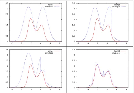
To construct the envelope, we start by considering the point u0 = c (c is required to be a point of the envelope in this algorithm). Then, the initial envelope is given by

(19) q(u) =q₋c (u) 1[u<c]+q+c (u) 1[c≤u]

We have successfully bounded hx,t from above with a piece-wise function formed by the

kernels of a Gaussian density times nite constants. Using the bounds (17) and (18) it is possible to rene q(u) by adding more points to it too. We illustrate the results of this procedure in Figure 1. If α is sub-linear, a dierent construction of q results in a tighter

envelope for the same number of points.

Considerable attention has been put in the implementation of an ecient algorithm to sample from ARS1:

(1) a binary search is performed (instead of a sequential one) to sample the interval of the piece-wise proposal q;

(2) the same uniform variate used to sample the interval is used to sample from the proper truncated Gaussian distribution by the cdf inversion method;

0 0.5 1 1.5 2 2.5 3 3.5

-2 0 2 4 6 8

kernel envelope

0 0.5 1 1.5 2 2.5 3 3.5

-2 0 2 4 6 8

kernel envelope

0 0.5 1 1.5 2 2.5 3 3.5

-2 0 2 4 6 8

kernel envelope

0 0.5 1 1.5 2 2.5 3 3.5

-2 0 2 4 6 8

kernel envelope

Figure 1. The test kernelhx,t and the proposal qconstructed from condition

(E1) for a test function hx,t. Starting from quadrant IV going clockwise we

have the envelope constructed from 1, 2, 3 points and the envelope that satises an acceptance rate of 95%

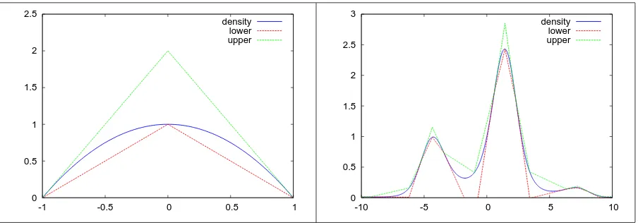
The second sampler, ARS2 from now on, has much weaker requirements of ARS1 and is of interest on its own. We basically require the function hx,t to be piece-wise twice

dieren-tiable and to exhibit an exponential decay in the tails. This sampler is a generalisation of the adaptive accept-reject sampler introduced in Gilks and Wild [1992], Gilks [1992]. We partition the state space Xinto intervals wherehx,t is convex/concave and use the geometric

interpretation of convexity to construct linear bounds above and below hx,t. We illustrate

the results of this procedure in Figures 2 and 3.

Similarly to the case of ARS1, considerable attention has been put in the implementation of an ecient algorithm to sample from ARS2. A brief simulation study in Peluchetti [2007] reveals that the eciency of ARS2 is comparable to that of the Gnu Scientic Library's ad-hoc samplers. ARS1, while somewhat less ecient, is a more robust sampler as it targets a very specic family of densities.

We now consider the more general problem of sampling from {hx,t(u)}_x∈X. Our idea is

0 0.5 1 1.5 2 2.5

-1 -0.5 0 0.5 1

density lower upper

0 0.5 1 1.5 2 2.5 3

-10 -5 0 5 10

density lower upper

Figure 2. The initial construction of the ARS2 on a single interval (left) and on the test density (right)

0 0.5 1 1.5 2 2.5

-1 -0.5 0 0.5 1

density lower upper

0 0.5 1 1.5 2 2.5 3

-10 -5 0 5 10

density lower upper

Figure 3. The rened construction of the ARS2 on a single interval (left) and on the test density (right)

preliminary simulation, into a nite number of equi-spaced intervals. For each interval, we construct an envelope that uniformly bounds all the hx,t whose x is a point of this interval.

To nd this uniform bound we notice that for l < r∈_X

sup

l≤x≤r

hx,t = sup l≤x≤r

eA(u)−(u−x2t)2 1

[u<l]+ 1[l≤u≤r]+ 1[r<u] (20)

≤eA(u)−(u−l2t)21_[u<l]+eA(u)1_[l≤u≤r]+eA(u)−

(u−r)2 2t 1_[r<u]

(21)

≤eA(u)−(u−l2t)21

[u<l]+eAmax1[l≤u≤r]+eA(u)−

(u−r)2 2t 1

[r<u] (22)

where Amax = sup_l≤u≤rA(u) < ∞ as A is a continuous function on a bounded interval,

hence A is bounded. The rst and the last term of (22) can be easily bounded by envelopes

accept-reject sampling algorithm whose acceptance rate is high if the length of the intervals is reasonably short. We thus pre-compute and cache all these uniform envelopes, one for each intervals in which we split D. During the simulation according to EA, if x ∈ D we select the right envelope, otherwise (an event whose probability can be arbitrarily small increasing D) we create an envelope accordingly. As the intervals are equi-spaced there is virtually no eciency penalty in searching for the right envelope.

2.3. The discretisation schemes. We now shortly introduce the three discretisation schemes (DS) whose eciency, with that of EA, is investigated in the simulation study. All the DSs are assumed to have an equi-spaced discretisation interval of length ∆ =T /n, where nis the

number of steps and Y∆ denotes a corresponding generic DS. In the following _{i = 1,· · · , n} and Y0 =x implicitly.

The Euler scheme is the simplest DS that can be used to approximate the solution of (1). It can be dened by the recursion

W_∆i iid∼ N (0,∆) (23)

Yi∆=Y(i−1)∆+b Y(i−1)∆

∆ +σ Y(i−1)∆

W_∆i

(24)

The Predictor-Corrector scheme is dened by

W_∆i iid∼ N (0,∆) (25)

Yi∆=Y(i−1)∆+b Y(i−1)∆

∆ +σ Y(i−1)∆

W_∆i

(26)

Yi∆=Y(i−1)∆+

1 2

b Y(i−1)∆

+b Yi∆ ∆ +σ Y(i−1)∆

W_∆i

(27)

The idea behind this DS is to make a Euler prediction _Y¯

i∆ by using (26) and adjust Y¯i∆ by computing an average of the drift's value over the time step((i−1) ∆, i∆]using the trapezoid quadrature formula. This approach results in the correction (27). It is fundamental to use the sameW_∆i in (26) and (27). For more details about the Euler and the Predictor-Corrector

schemes see Kloeden and Platen [1992].

Finally we introduce the Ozaki-Shoji scheme. This DS uses a completely dierent approach that is only applicable to diusion process with constant diusion coecient and, without loss of generality, to (3). This DS belongs to the family of "linearisation schemes" which approximates the drift α of (3) by some sort of linear approximation. The specic version

here presented it the one of Shoji and Ozaki [1998]. The idea behind this DS is to approximate the behaviour of α(Xt) in a neighbourhood of Xt using Ito's Lemma

dα(Xt) =α0(Xt)dXt+

1 2α

00_(X

t)dt

(28)

α(Xt+h)≈α(Xt) +α0(Xt) (Xt+h−Xt) +

1 2α

00

(Xt)h

The law of the Ozaki-Shoji scheme on the time interval (0,∆]is given by the solution of the linear SDE

(30) dXt=

α(x) +α0(x) (Xt−x) +

1 2α

00

(x)t

dt+dBt

i.e. a Gaussian process. By the time-homogeneity this DS is dened by the iterative formulae

˜

W_∆i iid∼ N 0,exp

2α0 Y(i−1)∆

∆ −1

2α0 _Y (i−1)∆

!

(31)

Yi∆=Y(i−1)∆+

α Y(i−1)∆

α0 _Y (i−1)∆

exp

α0 Y(i−1)∆

∆ −1 (32)

+ α

00

Y(i−1)∆

2 α0 _Y (i−1)∆

2

expα0 Y(i−1)∆

∆ −1−α0 Y(i−1)∆

∆ + ˜W_∆i

(33)

3. A simulation study

A standard way to compare DSs is related to the concepts of weak and strong convergence.

Y∆ _{is said to be a strong approximation of (1) if∃∆}∗_{, k,S >0 :∀∆≤∆}∗

(34) EX_T −Y_T∆

≤k∆S

where S is the rate of convergence. This strong converge criterion basically states the L1 convergence of the last simulated pointY∆

T toXT. As such, the rateS is an indicator of how

wellY∆ _{approximates the paths of X (for a xedω). The convergence is not uniform on the} time interval [0, T] and the leading order constantk depends on (1).

Y∆ _{is said to be a weak approximation of (1) if ∃∆}∗_{, k,W >0 :∀∆≤∆}∗_{, g ∈ G}

(35)

E[g(X_T)]−E

g Y_T∆≤k∆W

where W is the rate of weak convergence and G is a class of test functions. Here the rate W is an indicator of how accurately the distribution of Y∆ _{approximates the distribution of}

X. Hence this convergence criterion is more indicated if we are interested in Monte Carlo

simulations based on Y∆_{. Similarly to (34) the convergence in not uniform on [0, T]and the} constant k of (35) depends on the SDE (1), limiting the practical appeal of these criteria.

Our empirical results shows that DSs with the same W can perform very dierently.

The framework of the simulation study is very simple: we consider a unit diusion coe-cient SDEX (3) and a functionalF, possibly path-dependent, of interest. In this framework

we compare the eciency of EA and the three DSs previously introduced.

As EA does not clearly involves any discretisation error, its eciency is inversely pro-portional to the average computational cost required to sample a single realisation of the functional F (X).

For a givenY∆, the smallest computational cost, i.e. the biggest∆, required forF Y∆to

be an accurate approximation of F (X) is then computed. More precisely, we are interested in how similar the distribution of F Y∆

exactly. Let α ∈ (0,1) be a xed threshold and ∆∗ be the biggest value of ∆ such that the p-value of the KS test of

F (X), F Y∆ is higher then the threshold α. The eciency

of Y∆ _{is then dened as inversely proportional to the computational cost required for the} simulation of a single realisation of the functional F Y∆∗

. To compute the KS test of

F(X), F Y∆ _{we choose to sample N ∈}

N skeletons from

X using EA and N discretisation using Y∆. For each one of these samples the value of the

functional F is computed resulting in 2N samples: N exact and N approximated

observa-tions. Finally the p-value of the KS statistic calculated over these 2N samples. Moreover

to decrease the variance of the KS test (that in this framework is just stochastic noise) we average its value over M ∈ _N repetitions. All these simulations needs to be repeated until

we nd the right ∆∗ for each of the three DSs considered in the comparison, i.e. the smallest ∆ so that we accept the null hypothesis according to the KS test. Finally we repeat all these steps for a reasonable number of combinations of the parameters of the SDE, to obtain computational cost surfaces (as a function of the parameters) for EA and the DSs.

In our simulation study the following arbitrary values are considered: α = 0.05, N = 105, M = 103. The choice of the KS test is arbitrary too, but there are a number of reasons

why we opted for the this test. First of all, it has an intuitive meaning. More importantly, it is possible to obtain the limiting distribution of the KS statistic under the null hypothesis. Lastly we want to be cautious about our conclusions. The use of a more powerful goodness of t test would pose questions about the robustness of our results to the choice of the test statistic considered. This would be especially true for tests that give more importance to the tails of the distribution, as preliminary examination of the histograms of the densities involved reveals that the biggest dierences are usually in the tails.

The aim of this simulation study is to obtain useful indication about the eciency of EA and the three DSs. The choice of the diusion models that we take into account reects this objective, they are "toy examples".

3.1. The case of EA1. The class of parametric diusion models that can be considered is limited by the assumptions of EA1. We focus on the following three models:

• The PSINE SDE

dXt=θsin (γXt)dt+dBt θ > 0, γ >0

(36)

• The NSINE SDE

dXt=θsin (γXt)dt+dBt θ < 0, γ >0

(37)

• The PTANH SDE

dXt =θtanh (γXt)dt+dBt θ >0, γ >0

(38)

• The NTANH SDE

dXt =θtanh (γXt)dt+dBt θ <0, γ >0

We take into account these models because they summarise a good range of diusion dy-namics. In every model the starting point x and the terminal time T are xed to 0 and 1 respectively.

The functionals considered are the last point L(X) = XT and the maximum of the path M(X) = sup_0≤s≤T Xs. For M(X) we simulate the maximum of a BB between each

dis-cretized value even when dealing with DSs.

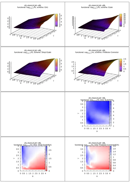
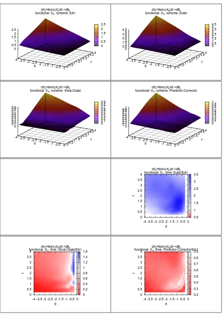
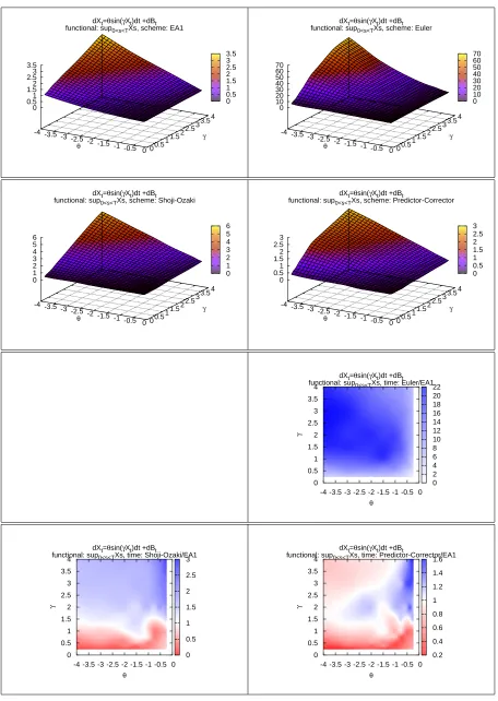
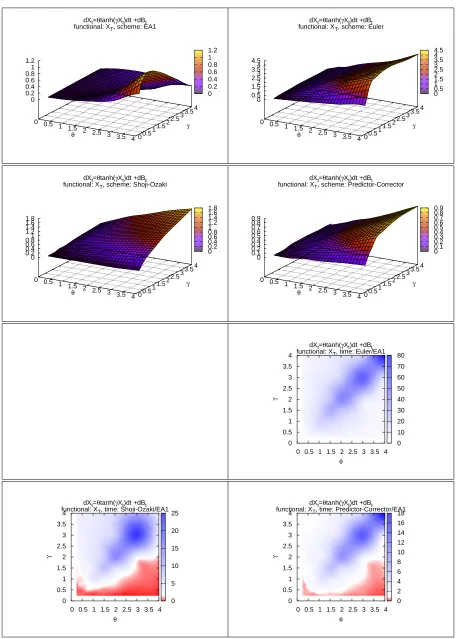
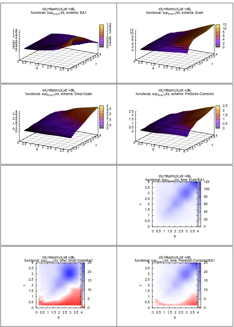
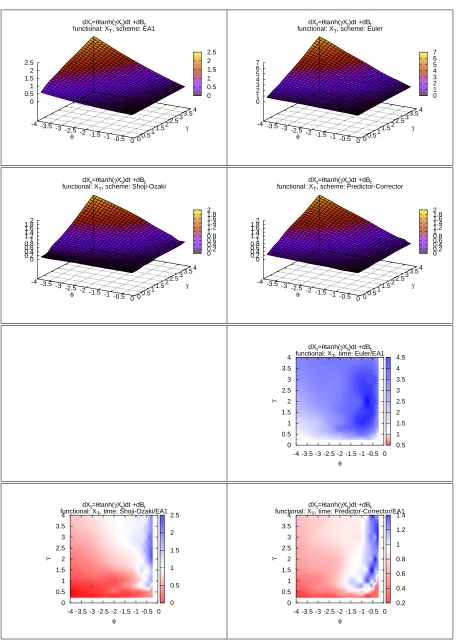
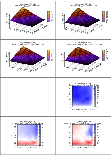
In Figures 4 to 11 the four plots on the top of each gure represents on the Z-axis the computational time required by EA and by the three DSs to complete the simulation (with the required level of accuracy) as function of the values of the SDE's parameters.

In the remaining 3 plots of each gure, the ratio of the computational time of a DS over the computational time of EA is represented on the Z-axis, again as a function of the SDE's parameters. Whenever possible, the white colour represents a unitary ratio, the red colour a ratio lower than1and the blue colour a ratio higher than1. We remark that these ratios are the results of our arbitrary choices. For example comparing a higher number of observations would increase the power of the test and this would result in a lower eciency of the DSs.

Moreover the shape of these surfaces is of interest on its own, as it says how the DSs behave with respect to parametric classes of drift and diusion coecients. From this point of view EA is a valuable validation tool.

The two main goals of this simulation are: commenting the eciency of EA with respect to other DSs and study the behaviour of EA and of the DSs with respect to qualitative characteristics of the diusion model X. Regarding the rst of these points, we note that:

(1) EA1 has a computational cost that is comparable to that of good DSs such as the Predictor-Corrector scheme. This means that there is generally not a huge dierence between simulating from the approximated or the exact law of the process.

(2) EA1 is favoured when we consider the functional M(X). One possible explanation for this is that while simulatingL(X)the discretisation errors of every step are likely to cancel, but when simulatingM(X)the errors are likely to accumulate. Moreover, we are using two levels of approximations: we approximate the discretized path and also the maximum of the path conditionally on the discretisation.

(3) While all DSs share a very good performance when γ is very low, independently of

the value of θ, this is not the case with EA1. While the computational cost in EA1

remains very contained it increases with |θ| more rapidly. Conversely, EA1 has a

better eciency than DSs when|θ| is low.

(4) There are situations where EA1 performs much better, and this is the case of the PTANH model. This happens because if α2 = α0 in (3) it follows that EA always

accept the proposed skeleton. In this case we actually know the transition density of X. This is the case when γ = θ in the PTANH. When we move away from the

diagonal the range of α2 +α0 increases and so does the rejection rate.

0 0.5 1 1.5 2 2.5 dXt=θsin(γXt)dt +dBt

functional: XT, scheme: EA1

0 0.5 _{1 1.5} 2 2.5

3 3.5 ₄

θ 0 0.5 1 1.5

2 2.5 3 3.5

4 γ 0 0.5 1 1.5 2 2.5 0 0.5 1 1.5 2 2.5 3 dXt=θsin(γXt)dt +dBt

functional: XT, scheme: Euler

0 0.5 _{1 1.5} 2 2.5

3 3.5 ₄

θ 0 0.5 1 1.5

2 2.5 3 3.5

4

γ

0 0.5 1 1.5 2 2.5 3

0 0.1 0.2 0.3 0.4 0.5 0.6 0.7 0.8 dX_t=θsin(γX_t)dt +dB_t

functional: X_T, scheme: Shoji-Ozaki

0 0.5

1 1.5 _{2 2.5} 3 3.5 ₄

θ 0 0.5 1 1.5

2 2.5 3 3.5

4 γ 0 0.1 0.2 0.3 0.4 0.5 0.6 0.7 0.8 0 0.1 0.2 0.3 0.4 0.5 0.6 0.7 0.8 dX_t=θsin(γX_t)dt +dB_t

functional: X_T, scheme: Predictor-Corrector

0 0.5

1 1.5 _{2 2.5} 3 3.5 ₄

θ 0 0.5 1 1.5

2 2.5 3 3.5

4 γ 0 0.1 0.2 0.3 0.4 0.5 0.6 0.7 0.8 0.5 1 1.5 2 2.5 3 dXt=θsin(γXt)dt +dBt functional: XT, time: Euler/EA1

0 0.5 1 1.5 2 2.5 3 3.5 4

θ 0 0.5 1 1.5 2 2.5 3 3.5 4 γ 0 0.2 0.4 0.6 0.8 1 1.2 1.4 1.6 dXt=θsin(γXt)dt +dBt

functional: XT, time: Shoji-Ozaki/EA1

0 0.5 1 1.5 2 2.5 3 3.5 4 γ 0.1 0.2 0.3 0.4 0.5 0.6 0.7 0.8 dXt=θsin(γXt)dt +dBt

functional: XT, time: Predictor-Corrector/EA1

0 0.5 1 1.5 2 2.5 3 3.5 4 dXt=θsin(γXt)dt +dBt

functional: sup0<s<TXs, scheme: EA1

0 0.5 _{1 1.5} 2 2.5

3 3.5 ₄

θ 0 0.5 1 1.5

2 2.5 3 3.5

4

γ

0 0.5 1 1.5 2 2.5 3 3.5 4

0 5 10 15 20 25 30 35 dXt=θsin(γXt)dt +dBt

functional: sup0<s<TXs, scheme: Euler

0 0.5 _{1 1.5} 2 2.5

3 3.5 ₄

θ 0 0.5 1 1.5

2 2.5 3 3.5

4 γ 0 5 10 15 20 25 30 35 0 0.5 1 1.5 2 2.5 3 3.5 4 dX_t=θsin(γX_t)dt +dB_t

functional: sup_0<s<TXs, scheme: Shoji-Ozaki

0 0.5

1 1.5 _{2 2.5} 3 3.5 ₄

θ 0 0.5 1 1.5

2 2.5 3 3.5

4

γ

0 0.5 1 1.5 2 2.5 3 3.5 4

0 0.5 1 1.5 2 2.5 dX_t=θsin(γX_t)dt +dB_t

functional: sup_0<s<TXs, scheme: Predictor-Corrector

0 0.5

1 1.5 _{2 2.5} 3 3.5 ₄

θ 0 0.5 1 1.5

2 2.5 3 3.5

4 γ 0 0.5 1 1.5 2 2.5 1 2 3 4 5 6 7 8 dXt=θsin(γXt)dt +dBt functional: sup0<s<TXs, time: Euler/EA1

0 0.5 1 1.5 2 2.5 3 3.5 4

θ 0 0.5 1 1.5 2 2.5 3 3.5 4 γ 0 0.5 1 1.5 2 2.5 3 dXt=θsin(γXt)dt +dBt

functional: sup0<s<TXs, time: Shoji-Ozaki/EA1

0 0.5 1 1.5 2 2.5 3 3.5 4 γ 0 0.2 0.4 0.6 0.8 1 1.2 1.4 1.6 1.8 dXt=θsin(γXt)dt +dBt

functional: sup0<s<TXs, time: Predictor-Corrector/EA1

0 0.5 1 1.5 2 2.5 dXt=θsin(γXt)dt +dBt

functional: XT, scheme: EA1

-4 -3.5 _{-3 -2.5} -2 -1.5

-1 -0.5 ₀

θ 0 0.5 1 1.5

2 2.5 3 3.5

4 γ 0 0.5 1 1.5 2 2.5 0 0.5 1 1.5 2 2.5 3 3.5 4 4.5 dXt=θsin(γXt)dt +dBt

functional: XT, scheme: Euler

-4 -3.5 _{-3 -2.5} -2 -1.5

-1 -0.5 ₀

θ 0 0.5 1 1.5

2 2.5 3 3.5

4

γ

0 0.5 1 1.5 2 2.5 3 3.5 4 4.5 0 0.1 0.2 0.3 0.4 0.5 0.6 0.7 0.8 0.9 dX_t=θsin(γX_t)dt +dB_t

functional: X_T, scheme: Shoji-Ozaki

-4 -3.5

-3 -2.5_{-2 -1.5} -1 -0.5 ₀

θ 0 0.5 1 1.5

2 2.5 3 3.5

4 γ 0 0.1 0.2 0.3 0.4 0.5 0.6 0.7 0.8 0.9 0 0.1 0.2 0.3 0.4 0.5 0.6 0.7 0.8 0.9 1 dX_t=θsin(γX_t)dt +dB_t

functional: X_T, scheme: Predictor-Corrector

-4 -3.5

-3 -2.5_{-2 -1.5} -1 -0.5 ₀

θ 0 0.5 1 1.5

2 2.5 3 3.5

4 γ 0 0.1 0.2 0.3 0.4 0.5 0.6 0.7 0.8 0.9 1

0.5 1 1.5 2 2.5 3 3.5 dXt=θsin(γXt)dt +dBt

functional: XT, time: Euler/EA1

-4 -3.5 -3 -2.5 -2 -1.5 -1 -0.5 0

θ 0 0.5 1 1.5 2 2.5 3 3.5 4 γ 0 0.2 0.4 0.6 0.8 1 1.2 1.4 1.6 dXt=θsin(γXt)dt +dBt

functional: XT, time: Shoji-Ozaki/EA1

0 0.5 1 1.5 2 2.5 3 3.5 4 γ 0.2 0.3 0.4 0.5 0.6 0.7 0.8 0.9 dXt=θsin(γXt)dt +dBt

functional: XT, time: Predictor-Corrector/EA1

0 0.5 1 1.5 2 2.5 3 3.5 dXt=θsin(γXt)dt +dBt

functional: sup0<s<TXs, scheme: EA1

-4 -3.5 _{-3 -2.5} -2 -1.5

-1 -0.5 ₀

θ 0 0.5 1 1.5

2 2.5 3 3.5

4

γ

0 0.5 1 1.5 2 2.5 3 3.5 0 10 20 30 40 50 60 70 dXt=θsin(γXt)dt +dBt

functional: sup0<s<TXs, scheme: Euler

-4 -3.5 _{-3 -2.5} -2 -1.5

-1 -0.5 ₀

θ 0 0.5 1 1.5

2 2.5 3 3.5

4 γ 0 10 20 30 40 50 60 70 0 1 2 3 4 5 6 dX_t=θsin(γX_t)dt +dB_t

functional: sup_0<s<TXs, scheme: Shoji-Ozaki

-4 -3.5

-3 -2.5_{-2 -1.5} -1 -0.5 ₀

θ 0 0.5 1 1.5

2 2.5 3 3.5

4 γ 0 1 2 3 4 5 6 0 0.5 1 1.5 2 2.5 3 dX_t=θsin(γX_t)dt +dB_t

functional: sup_0<s<TXs, scheme: Predictor-Corrector

-4 -3.5

-3 -2.5_{-2 -1.5} -1 -0.5 ₀

θ 0 0.5 1 1.5

2 2.5 3 3.5

4 γ 0 0.5 1 1.5 2 2.5 3 0 2 4 6 8 10 12 14 16 18 20 22 dXt=θsin(γXt)dt +dBt

functional: sup0<s<TXs, time: Euler/EA1

-4 -3.5 -3 -2.5 -2 -1.5 -1 -0.5 0

θ 0 0.5 1 1.5 2 2.5 3 3.5 4 γ 0 0.5 1 1.5 2 2.5 3 dXt=θsin(γXt)dt +dBt

functional: sup0<s<TXs, time: Shoji-Ozaki/EA1

0 0.5 1 1.5 2 2.5 3 3.5 4 γ 0.2 0.4 0.6 0.8 1 1.2 1.4 1.6 dXt=θsin(γXt)dt +dBt

functional: sup0<s<TXs, time: Predictor-Corrector/EA1

0 0.2 0.4 0.6 0.8 1 1.2 dXt=θtanh(γXt)dt +dBt

functional: XT, scheme: EA1

0 0.5 _{1 1.5} 2 2.5

3 3.5 ₄

θ 0 0.5 1 1.5

2 2.5 3 3.5

4 γ 0 0.2 0.4 0.6 0.8 1 1.2 0 0.5 1 1.5 2 2.5 3 3.5 4 4.5 dXt=θtanh(γXt)dt +dBt

functional: XT, scheme: Euler

0 0.5 _{1 1.5} 2 2.5

3 3.5 ₄

θ 0 0.5 1 1.5

2 2.5 3 3.5

4

γ

0 0.5 1 1.5 2 2.5 3 3.5 4 4.5 0 0.2 0.4 0.6 0.8 1 1.2 1.4 1.6 1.8 dX_t=θtanh(γX_t)dt +dB_t

functional: X_T, scheme: Shoji-Ozaki

0 0.5

1 1.5 _{2 2.5} 3 3.5 ₄

θ 0 0.5 1 1.5

2 2.5 3 3.5

4 γ 0 0.2 0.4 0.6 0.8 1 1.2 1.4 1.6 1.8 0 0.1 0.2 0.3 0.4 0.5 0.6 0.7 0.8 0.9 dX_t=θtanh(γX_t)dt +dB_t

functional: X_T, scheme: Predictor-Corrector

0 0.5

1 1.5 _{2 2.5} 3 3.5 ₄

θ 0 0.5 1 1.5

2 2.5 3 3.5

4 γ 0 0.1 0.2 0.3 0.4 0.5 0.6 0.7 0.8 0.9 0 10 20 30 40 50 60 70 80 dXt=θtanh(γXt)dt +dBt functional: XT, time: Euler/EA1

0 0.5 1 1.5 2 2.5 3 3.5 4

θ 0 0.5 1 1.5 2 2.5 3 3.5 4 γ 0 5 10 15 20 25 dXt=θtanh(γXt)dt +dBt functional: XT, time: Shoji-Ozaki/EA1

0 0.5 1 1.5 2 2.5 3 3.5 4 γ 0 2 4 6 8 10 12 14 16 18 dXt=θtanh(γXt)dt +dBt functional: XT, time: Predictor-Corrector/EA1

0 0.2 0.4 0.6 0.8 1 1.2 1.4 1.6 1.8 dXt=θtanh(γXt)dt +dBt

functional: sup0<s<TXs, scheme: EA1

0 0.5 _{1 1.5} 2 2.5

3 3.5 ₄

θ 0 0.5 1 1.5

2 2.5 3 3.5

4 γ 0 0.2 0.4 0.6 0.8 1 1.2 1.4 1.6 1.8 0 2 4 6 8 10 12 dXt=θtanh(γXt)dt +dBt

functional: sup0<s<TXs, scheme: Euler

0 0.5 _{1 1.5} 2 2.5

3 3.5 ₄

θ 0 0.5 1 1.5

2 2.5 3 3.5

4 γ 0 2 4 6 8 10 12 0 0.5 1 1.5 2 2.5 3 3.5 4 dX_t=θtanh(γX_t)dt +dB_t

functional: sup_0<s<TXs, scheme: Shoji-Ozaki

0 0.5

1 1.5 _{2 2.5} 3 3.5 ₄

θ 0 0.5 1 1.5

2 2.5 3 3.5

4

γ

0 0.5 1 1.5 2 2.5 3 3.5 4

0 0.5 1 1.5 2 2.5 dX_t=θtanh(γX_t)dt +dB_t

functional: sup_0<s<TXs, scheme: Predictor-Corrector

0 0.5

1 1.5 _{2 2.5} 3 3.5 ₄

θ 0 0.5 1 1.5

2 2.5 3 3.5

4 γ 0 0.5 1 1.5 2 2.5 0 20 40 60 80 100 120 dXt=θtanh(γXt)dt +dBt

functional: sup0<s<TXs, time: Euler/EA1

0 0.5 1 1.5 2 2.5 3 3.5 4

θ 0 0.5 1 1.5 2 2.5 3 3.5 4 γ 0 5 10 15 20 25 dXt=θtanh(γXt)dt +dBt

functional: sup0<s<TXs, time: Shoji-Ozaki/EA1

0 0.5 1 1.5 2 2.5 3 3.5 4 γ 0 5 10 15 20 25 dXt=θtanh(γXt)dt +dBt

functional: sup0<s<TXs, time: Predictor-Corrector/EA1

0 0.5 1 1.5 2 2.5 dXt=θtanh(γXt)dt +dBt

functional: XT, scheme: EA1

-4 -3.5 _{-3 -2.5} -2 -1.5

-1 -0.5 ₀

θ 0 0.5 1 1.5

2 2.5 3 3.5

4 γ 0 0.5 1 1.5 2 2.5 0 1 2 3 4 5 6 7 dXt=θtanh(γXt)dt +dBt

functional: XT, scheme: Euler

-4 -3.5 _{-3 -2.5} -2 -1.5

-1 -0.5 ₀

θ 0 0.5 1 1.5

2 2.5 3 3.5

4 γ 0 1 2 3 4 5 6 7 0 0.2 0.4 0.6 0.8 1 1.2 1.4 1.6 1.8 2 dX_t=θtanh(γX_t)dt +dB_t

functional: X_T, scheme: Shoji-Ozaki

-4 -3.5

-3 -2.5_{-2 -1.5} -1 -0.5 ₀

θ 0 0.5 1 1.5

2 2.5 3 3.5

4 γ 0 0.2 0.4 0.6 0.8 1 1.2 1.4 1.6 1.8 2

0 0.2 0.4 0.6 0.8 1 1.2 1.4 1.6 1.8 2 dX_t=θtanh(γX_t)dt +dB_t

functional: X_T, scheme: Predictor-Corrector

-4 -3.5

-3 -2.5_{-2 -1.5} -1 -0.5 ₀

θ 0 0.5 1 1.5

2 2.5 3 3.5

4 γ 0 0.2 0.4 0.6 0.8 1 1.2 1.4 1.6 1.8 2

0.5 1 1.5 2 2.5 3 3.5 4 4.5 dXt=θtanh(γXt)dt +dBt

functional: XT, time: Euler/EA1

-4 -3.5 -3 -2.5 -2 -1.5 -1 -0.5 0

θ 0 0.5 1 1.5 2 2.5 3 3.5 4 γ 0 0.5 1 1.5 2 2.5 dXt=θtanh(γXt)dt +dBt

functional: XT, time: Shoji-Ozaki/EA1

0 0.5 1 1.5 2 2.5 3 3.5 4 γ 0.2 0.4 0.6 0.8 1 1.2 1.4 dXt=θtanh(γXt)dt +dBt

functional: XT, time: Predictor-Corrector/EA1

0 0.5 1 1.5 2 2.5 3 3.5 dXt=θtanh(γXt)dt +dBt

functional: sup0<s<TXs, scheme: EA1

-4 -3.5 _{-3 -2.5} -2 -1.5

-1 -0.5 ₀

θ 0 0.5 1 1.5

2 2.5 3 3.5

4

γ

0 0.5 1 1.5 2 2.5 3 3.5 0 10 20 30 40 50 60 70 dXt=θtanh(γXt)dt +dBt

functional: sup0<s<TXs, scheme: Euler

-4 -3.5 _{-3 -2.5} -2 -1.5

-1 -0.5 ₀

θ 0 0.5 1 1.5

2 2.5 3 3.5

4 γ 0 10 20 30 40 50 60 70 0 0.5 1 1.5 2 2.5 3 3.5 4 4.5 5 5.5 dX_t=θtanh(γX_t)dt +dB_t

functional: sup_0<s<TXs, scheme: Shoji-Ozaki

-4 -3.5

-3 -2.5_{-2 -1.5} -1 -0.5 ₀

θ 0 0.5 1 1.5

2 2.5 3 3.5

4

γ

0 0.5 1 1.5 2 2.5 3 3.5 4 4.5 5 5.5 0 0.5 1 1.5 2 2.5 3 dX_t=θtanh(γX_t)dt +dB_t

functional: sup_0<s<TXs, scheme: Predictor-Corrector

-4 -3.5

-3 -2.5_{-2 -1.5} -1 -0.5 ₀

θ 0 0.5 1 1.5

2 2.5 3 3.5

4 γ 0 0.5 1 1.5 2 2.5 3 0 2 4 6 8 10 12 14 16 18 20 dXt=θtanh(γXt)dt +dBt functional: sup0<s<TXs, time: Euler/EA1

-4 -3.5 -3 -2.5 -2 -1.5 -1 -0.5 0

θ 0 0.5 1 1.5 2 2.5 3 3.5 4 γ 0 0.5 1 1.5 2 2.5 3 3.5 dXt=θtanh(γXt)dt +dBt

functional: sup0<s<TXs, time: Shoji-Ozaki/EA1

0 0.5 1 1.5 2 2.5 3 3.5 4 γ 0.2 0.4 0.6 0.8 1 1.2 1.4 1.6 1.8 dXt=θtanh(γXt)dt +dBt

functional: sup0<s<TXs, time: Predictor-Corrector/EA1

(1) Euler scheme is clearly the least ecient DS. In some situation it can be 20 times more inecient than the other two DSs. Moreover the implementation diculty o all these DSs is comparable.

(2) Predictor-Corrector and Ozaki-Shoji scheme shares more or less the same eciency, even if in the same situations the former can be two times more ecient than the latter. Furthermore, the Ozaki-Shoji scheme exhibits numerical instabilities every time α0 Y(i−1)∆

≈ 0. Hence it is necessary to introduce an extra check for the algorithm that would slow down the simulation even more. All this suggests that the Predictor-Corrector scheme should be the rst choice in most situations.

(3) As already stated, the weak convergence criterion is not very useful from a practitioner point of view. In fact both the Euler DS and the Predictor-Corrector DS share the same unit-order of weak convergence.

(4) It is very dicult with this limited amount of information to infer a rule of thumbs that links the eciency of the DSs to the qualitative behaviour of the target diusion model X. We just notice that the computational time surface has more or less the

same shape in all the DSs. The dierence is in the multiplicative factor.

3.2. The case of EA3. We consider the following diusion models

• the LANG SDE

dXt=−ksign(Xt)|Xt|βdt+dBt k >0, β ∈N (40)

• the XXCUBE SDE

dXt=

−αX_t3+βXt dt+dBt α >0, β >0

(41)

In the case of EA3, we can no longer easily and exactly simulate from the law of M(X), hence the comparison is only limited to the L(X) functional. As the results of Section 3.1 suggests that Shoji-Ozaki scheme does not oer any clear advantage against Predictor-Corrector scheme, while showing numerical instabilities, we decide to include the Euler DS and the Predictor-Corrector DS in the comparison only.

Regarding the eciency of EA3 with respect to Predictor-Corrector scheme we notice that the former is always less ecient then the the latter. The most obvious reason is that EA3 is much more complicated from an algorithmic point of view than EA1, and this results in a higher computational time. However, everything is relative to the choice of the specic comparison criterion considered. As a rule of thumb we can say that EA3 is a factor of 10 slower than EA1.

Given these results, there is no obvious link between qualitative behaviour of the diusion model X and the expected eciency of the DSs. The relative eciency of Euler with respect

0 0.5 1 1.5 2 2.5 3 dXt=-κsgn(Xt)|Xt|βdt +dBt

functional: XT, scheme: EA3

0 _0.5 1 _1.5

2 _2.5 3

κ 1 1.5

2 2.5

3

β

0 0.5 1 1.5 2 2.5 3

0 0.1 0.2 0.3 0.4 0.5 0.6 0.7 0.8 dX_t=-κsgn(X_t)|X_t|βdt +dB_t

functional: X_T, scheme: Euler

0 _0.5 1 _1.5

2 _2.5 3

κ 1 1.5

2 2.5

3

β

0 0.1 0.2 0.3 0.4 0.5 0.6 0.7 0.8

0 0.05 0.1 0.15 0.2 0.25 dX_t=-κsgn(X_t)|X_t|βdt +dB_t

functional: X_T, scheme: Predictor-Corrector

0 _0.5 1 _1.5

2 _2.5 3

κ 1 1.5

2 2.5

3

β

0 0.05 0.1 0.15 0.2 0.25

0.06 0.08 0.1 0.12 0.14 0.16 0.18 0.2 dXt=-κsgn(Xt)|Xt|βdt +dBt functional XT, time: Predictor-Corrector/EA3

0 0.5 1 1.5 2 2.5 3

θ

1 1.5 2 2.5 3

γ

0.1 0.2 0.3 0.4 0.5 0.6 0.7 0.8 0.9 dXt=-κsgn(Xt)|Xt|βdt +dBt functional XT, time: Euler/EA3

0 0.5 1 1.5 2 2.5 3

θ

1 1.5 2 2.5 3

γ

Figure 12. model: LANG, functional: L(X)

4. The multi-dimensional setting We now concentrate on the unit-diusion d-dimensional SDE

dXt =α(Xt)dt+dBt t∈[0, T]

(42)

0 2 4 6 8 10 12 14 dXt=(αXt - βXt

3 )dt +dBt functional: XT, scheme: EA3

0 _0.5 1 _1.5

2 _2.5 3

α 0 0.5 1 1.5

2 2.5 3 β 0 2 4 6 8 10 12 14 0 1 2 3 4 5 6 7 dX_t=(αX_t - βX_t3)dt +dB_t

functional: X_T, scheme: Euler

0 _0.5 1 _1.5

2 _2.5 3

α 0 0.5 1 1.5

2 2.5 3 β 0 1 2 3 4 5 6 7 0.05 0.1 0.15 0.2 0.25 0.3 0.35 0.4 0.45 dX_t=(αX_t - βX_t3)dt +dB_t

functional: X_T, scheme: Predictor-Corrector

0 _0.5 1 _1.5

2 _2.5 3

α 0 0.5 1 1.5

2 2.5 3

β

0.05 0.1 0.15 0.2 0.25 0.3 0.35 0.4 0.45 0.025 0.03 0.035 0.04 0.045 0.05 0.055 0.06 0.065 0.07 0.075 dXt=(αXt - βXt

3 )dt +dBt functional: XT, time: Predictor-Corrector/EA3

0 0.5 1 1.5 2 2.5 3

θ 0 0.5 1 1.5 2 2.5 3 γ 0.05 0.1 0.15 0.2 0.25 0.3 0.35 0.4 0.45 0.5 0.55 dXt=(αXt - βXt

3 )dt +dBt functional: XT, time: Euler/EA3

0 0.5 1 1.5 2 2.5 3

θ 0 0.5 1 1.5 2 2.5 3 γ

Figure 13. model: XXCUBE, functional: L(X)

where Bt is the d-dimensional BM. The drift coecient α is assumed to satisfy proper

It is possible to nd equivalent conditions to (C1)-(C4) for the d-dimensional framework

and we refer to Beskos et al. [2006b] for a formal development of EA in this setting. The main theoretical limitations of EA in the d-dimensional setting are:

(1) the necessary and sucient condition for the existence of a transformation from a genericd-dimensional SDE to the unit diusion coecient SDE (42) is quite

demand-ing (see Ait-Sahalia [2002]);

(2) we require the existence of a potential functionA:_Rd _→

Rsuch thatα(u) = ∇A(u). EA then generalises to this setting in a simple way. We dene the d-dimensional BBM Z as

a d-dimensional BM with initial valuexconditioned on having its nal value ZT distributed

according to hx,t(u) where

(43) hx,t(u)∝exp

A(u)−ku−xk

2

2T

and denote with ZxT its law. Let φ : X → R, assumed to be bounded below, be dened as φ(u) := (kα(u)k2 _{+divα(u))/2−l and l := inf}

r∈Xφ(r) < ∞. As before L denote the law of a unit rate Poisson Point Process (PPP) on [0, T]×[0,∞), and let Φ = {χ, ψ} be

distributed according to Φ. We dene the event Γ as

(44) Γ := \

j≥1

φ Zχj

≤ψj

The following extension of Theorem 1 holds

Theorem 2. (Multivariate Wiener-Poisson factorisation) If (Z,Φ) ∼ _Zx

T ⊗L | Γ

then Z ∼_Qx

T

Proof. see Beskos et al. [2006b]

Using Theorem 2, the extension of EA1 to the d-dimensional setting is immediate. The

only diculty is nding the global maximum of φ over the domain_X. The extension of EA3

to the d-dimensional setting is similarly immediate, with the added diculty that we now

have to compute the maximum of φ over a bounded d-dimensional hyper-rectangle in _X.

As in the case of the one-dimensional EA the simulation of Z requires to sample from {hx,T (u)}_x∈X. Unfortunately the high dimensionality of the problem makes any adaptive approach, such as the ones in Peluchetti [2007], infeasible. However, if we can nd a d

-dimensional matrix K, a vector v and a constant k such that

(1) ∀u∈_XA(u)≤(u−v)0K(u−v) +k

(2) _Xexpn(u−v)0K(u−v)− ku−_2Txk2o<∞

it is possible to implement a simple accept-reject sampler using a multivariate Gaussian variate as proposal (the LPS from now on). In most diusion models of interest it is possible to nd such K,v, k that satises these conditions (at least for T small enough) indeed.

To see how the computation cost of EA scales as d increases we considered two test d

Dimension 1 2 4 8 16 EA1 comp.cost 0.48 0.92 1.85 5.56 27.51

Table 1. The multi-dimensional EA1

Dimension 1 2 3 4 5 6 7 8 9 10 11

LPS acceptance 83.9 71.3 61.3 52.3 44.4 37.4 32.5 27.2 23.3 19.3 17.2 EA3 comp. cost 0.39 0.31 0.40 0.46 0.75 1.21 2.15 5.87 15.9 45.9 129.9

Table 2. The multi-dimensional EA3

• the d-dimensional SINE, A(u) =−cosPd_i=1ui

• the d-dimensional LANG, A(u) =−Pn_i=1u4_i

The initial value x is the origin of _Rd and T = 1. Theoretical consideration suggests that partitioning [0, T] in sub-intervals of lengthT /d (and applying EA sequentially) would keep

the acceptance rate of EA stable as d changes. Our simulation study suggests that this

intuition is correct and we adopt this strategy.

In Table 1 we report the computational cost (in seconds) required to sample1000 observa-tions from the d-dimensional SINE SDE using EA1. We see that, apart from variations due

to the implementation, the computational cost increases linearly with d. Due to the bounded

nature of this example the acceptance rate of the LPS is stable.

In Table 2 we report the computational cost of the d-dimensional EA3 required to sample

100 observations from the d-dimensional LANG SDE. While the acceptance rate of the LPS

decreases with d (as expected) this is not the reason of the explosive behaviour of the d

-dimensional EA3's computational cost. The problem is the computation of the maximum of over a bounded d-dimensional hyper-rectangle that requires at least 2d computations.

5. Conclusions

In this paper we have performed a simulation study of EA's eciency. We have investigated the computational time required by EA1 and EA3 in dierent scenarios, both in the one andd

In the case of EA3, the added complexity of the algorithm has resulted in a less ecient scheme. The choice of the suggested discretization schemes thus depends on the particu-lar application. When a very precise simulation is needed, EA3 still presents a reasonable eciency, being roughly a factor of 10 slower then EA1.

In the d-dimensional case EA1 scales quadratically with the dimension d, while in most

cases EA3 scales exponentially. However, the exact simulation of not too high-dimensional problems remains feasible.

Moreover, the exact nature of EA is of great importance when eciency is not the rst concern. Thanks to EA we have been able to analyse the eciency of other discretization schemes with a high degree of accuracy. And we did so by considering diusion models for which the exact solution is not available in a closed form. Another example of an application of EA as a validation tool is that of inference for diusion model. Some methods rely on Euler-like approximations of the diusion process. By using the Euler (or similar) discretization scheme again for generating paths to test the method would false the conclusions of the experiment.

Concerning the behaviour of the DSs with respect to the SDEs' parameters, the small amount of information collected is not sucient to establish any rule of thumb. Additional research is needed to gain more insight on this interesting topic.

References

Y. Ait-Sahalia. Closed-Form Likelihood Expansions for Multivariate Diusions. 2002. C. Albanese and A. Kuznetsov. Transformations of Markov processes and

clas-sication scheme for solvable driftless diusions. preprint, www3. imperial. ac. uk/mathn/people/calban/papersmathn, 2005.

A. Beskos and G.O. Roberts. Exact simulation of diusions. Ann. Appl. Probab, 15:2422 2444, 2005.

A. Beskos, O. Papaspiliopoulos, and G.O. Roberts. Retrospective exact simulation of diusion sample paths with applications. Bernoulli, 12:10771098, 2006a.

A. Beskos, O. Papaspiliopoulos, and G.O. Roberts. A new factorisation of diusion measure and nite sample path construction. Methodology and Computing in Applied Probability, Submitted, 2006b.

Bruno Casella. Exact MC simulation for diusion and jump-diusion processes with nancial applications. PhD thesis, IMQ - Bocconi University, 2005.

WR Gilks. Derivative-free adaptive rejection sampling for Gibbs sampling. Bayesian Statis-tics, 4(2):641649, 1992.

WR Gilks and P. Wild. Adaptive Rejection Sampling for Gibbs Sampling. Applied Statistics, 41(2):337348, 1992.

P.E. Kloeden and E. Platen. Numerical Solution of Stochastic Dierential Equations. Springer, 1992.

Stefano Peluchetti. An analysis of the eciency of the Exact Algorithm. PhD thesis, IMQ -Universitá Commerciale Luigi Bocconi, 2007.